Beyond Shocks: How ESG Fundamentals Shape Geopolitical Risk Across Countries

Abstract

This paper examines the connection between Environmental, Social, and Governance (ESG) factors and the risk of geopolitics, as defined by the Geopolitical Risk (GPR) index. The concept of geopolitical risk is conventionally defined as the direct result of political incidents, war, and international tensions. The current study argues that the concept should be understood in a more structural and sustainable manner, relating to the underlying forces driving geopolitical risk. The main research question is whether and how the three pillars of ESG factors contribute to explaining and understanding cross-country and over-time variations in geopolitical risk. In an effort to avoid information loss associated with the ESG index’s aggregate nature, the three factors are considered separately and the three pillars are analyzed individually. The empirical context is a balanced cross-country panel dataset including 42 countries over the 2000–2023 time period. Data for the three factors are obtained from the World Bank dataset to standardize and compare data across countries and over time. The GPR index measures the level of geopolitical risk and is defined by Dario Caldara and Matteo Iacoviello. The GPR index captures the level of geopolitical tensions by analyzing media signals. The combination of the three sources enables direct connections and correlations among the three factors and the internationally recognized GPR index. The paper uses an integrated methodological approach that combines results from three distinct methods. The first method uses panel data analysis to estimate average marginal effects while controlling for unobserved heterogeneity. The second method uses clustering to identify structural patterns and divide countries into groups based on their unique characteristics and risk profiles. The third method uses machine learning regressions and nonparametric analysis to capture the complex relationships and interactions in the data. The three-step method is used for each pillar to ensure consistency and comparability. The results suggest that the three factors contribute to the GPR index in a unique manner. The environment and energy structure contribute to the GPR index as a risk multiplier; the social factor relates to exposure to instability; and the governance factor is a central stabilizing factor. The paper makes a unique contribution to the literature by defining the three factors and their relationship to the GPR index in a clear, sustainable manner.

1. Introduction

In other words, geopolitical risk is one of the key defining characteristics of the global world order. Political instability, conflicts, and other issues have become major concerns for global financial markets and macroeconomic stability. Recent research on geopolitical risk suggests its measurable and dynamic nature, rather than its subjective nature, and its role in creating policy uncertainty and global spillovers (Caldara & Iacoviello, 2022; Caldara et al., 2020). On the other hand, Environmental, Social, and Governance (ESG) criteria have become critical measures of sustainable and systemic risks faced by countries grappling with climate change, social instability, and governance challenges (Bolton et al., 2020; Pedersen et al., 2021). Although ESG and geopolitical risk have become increasingly important for global financial markets and macroeconomic stability, research on them has been conducted separately. This research aims to bridge the research gap by examining whether ESG criteria explain variations in geopolitical risk across countries and over time. A large body of evidence suggests that geopolitical instability is often driven by structural factors such as environmental degradation, climate change, resource scarcity, inequality, and poor governance. Simultaneously, governance quality, through its impact on institutional quality, rule of law, and corruption management, is considered essential for determining a country’s ability to withstand internal and external risks (Acemoglu et al., 2011; Kaufmann, 2007; Kahn et al., 2021). However, existing research mostly considers these drivers individually and treats geopolitical risk as an external factor affecting economic stability. However, this paper takes a different approach and considers ESG factors as structural drivers of countries’ vulnerabilities/resilience to geopolitical instability. From a methodological perspective, the research is an important contribution to the existing literature for its use of a mixed-methods approach combining panel econometrics, clustering, and ML regressions. This approach allows for identifying linear and nonlinear relationships between ESG and geopolitical risk. Additionally, rather than using aggregate ESG scores, it considers each of the Environmental, Social, and Governance aspects separately, enabling more accurate analysis of these drivers. Overall, it is considered a new contribution to the existing literature due to its focus on a new approach to understanding geopolitical risk from a sustainability perspective and its new evidence on ESG and geopolitical risk.

Geopolitical Risk as an Internationally Interconnected Phenomenon. Although ESG metrics are measured at the national level, geopolitical risk is not considered an internally generated risk in the context of the current research. This is because the Geopolitical Risk (GPR) index incorporates global tensions, wars, diplomatic conflicts, terrorism, and overall international instability through the systematic analysis of global media coverage. This means the overall dependent variable essentially incorporates the spillovers and external shocks of geopolitical risk, including global energy crises, regional wars, strategic conflicts, and climatic shocks. Within the context of the current research, the overall ESG conditions are not considered drivers of internally generated geopolitical risk. Instead, they are considered the drivers of the overall structural conditions of resilience or vulnerability. This means geopolitical risk is the product of the interplay between global shocks and domestic structural conditions. This means ESG conditions are essentially considered mediating variables within the overall context of the international risk architecture.

Linking Research Objectives to the Empirical Strategy. To maintain consistency between the research objectives and the methodological approach, each methodological approach is directly related to a particular analytical objective. First, panel econometric models are used to estimate the average marginal effects of the Environmental, Social, and Governance pillars on geopolitical risk across countries and over time. This methodological approach directly relates to the main research objective of identifying statistically significant structural relationships while controlling for potential unobservable heterogeneity. Secondly, clustering methods are applied to identify potential latent structural regimes and classify countries according to ESG-based risk profiles, thereby directly addressing the second research objective of identifying heterogeneous sustainability-risk configurations. Thirdly, machine learning regression methods are applied to identify potential nonlinear relationships and intricate dependencies between ESG indicators and geopolitical risk, thereby directly addressing the third research objective: identifying patterns that may be overlooked in a linear context.

From Isolated Determinants to an ESG-Embedded Architecture of Geopolitical Risk. Significant research has been conducted to study the interdependencies of variables like climate change-conflict, governance quality-political stability, inequality-social unrest, etc. However, current models have largely focused on these variables individually or treated them as exogenous to amplify the impact of shocks. Similarly, variables such as climate change as a catalyst for conflict, governance quality as a driver of political instability, and inequality as a catalyst for social unrest, among others, have been the focus of many models. Although these models are informative, they are largely unidimensional, highlighting the individual impact of these variables rather than the comprehensive structure of underlying structural conditions. In this study, a conceptual shift is introduced in the treatment of Environmental, Social, and Governance (ESG) factors, suggesting that these factors constitute a comprehensive structure of underlying conditions rather than individual variables such as climate change, social stability, governance quality, etc. A broader perspective of risk emerges by analyzing the individual components of these factors. In this context, geopolitical risk arises from sustainability fundamentals, with the country’s exposure, sensitivity, and adaptability to global disturbances considered.

The remainder of the article is organized as follows. Section 2 presents the literature review, positioning the study within the existing research on ESG factors and geopolitical risk. Section 3 describes the methodological framework, outlining the integrated ESG-based multi-method approach adopted in the analysis. Section 4 examines the Environmental dimension of ESG and its relationship with geopolitical risk through panel models, clustering techniques, and machine learning methods. Section 5 analyzes the Social dimension, focusing on the social foundations of geopolitical risk within the ESG framework. Section 6 investigates the role of Governance as a structural driver of geopolitical risk from an ESG perspective. Section 7 provides an integrated discussion of the results, synthesizing the findings across the Environmental, Social, and Governance components. Section 8 discusses the policy and stakeholder implications, highlighting ESG-based strategies for enhancing geopolitical resilience. Section 9 addresses the main limitations of the empirical framework and the data constraints. Finally, Section 10 concludes the study. Appendix A reports the supervised machine learning model specifications and hyperparameter settings, Appendix B presents the panel model statistics and diagnostic tests, Appendix C lists the countries included in the analysis, and Appendix D provides the list of acronyms used throughout the study.

2. Literature Review

A considerable body of literature suggests that geopolitical risks (GPRs) should be considered not only as risk events but also as structural drivers of sustainability, finance, and institutions. Empirical evidence suggests that geopolitical risks affect ESG-related risks and sustainability (Benammar et al., 2026; Doğan & Zeren, 2025; Sovbetov, 2025). Major geopolitical risks, such as the Russia-Ukraine conflict and tensions among major world powers, have been identified as asymmetrically affecting ESG performance across economies (Boccaletti et al., 2026; Sha et al., 2025). A second group of studies focuses on financial/market mechanisms to connect geopolitical risks with ESG risks. Empirical evidence suggests that geopolitical risks affect ESG risks in finance/investments. Geopolitical risks in finance/investments lead to higher volatility in financial markets (Huo & Shi, 2025; Newaz & Aslam, 2025). A third group of studies focuses on environmental/energy mechanisms to connect sustainability with geopolitical risks. Empirical evidence suggests that ESG risks affect geopolitical risks through energy dependency and climate vulnerability (Das et al., 2026; Akadiri & Özkan, 2026; Li et al., 2026). At the same time, another group of studies on natural resources/environmental risks suggests that they can be systemic risk multipliers. Institutional governance factors are also recognized as key moderators of the ESG and geopolitical risk relationship. In this context, empirical evidence indicates that robust governance structures can mitigate geopolitical risks, while institutional failures can accentuate them (Kuai & Wang, 2025; Al Amosh & Khatib, 2025; Cheng et al., 2025). In this context, geopolitical risks are treated as endogenous variables that reflect structural economic and institutional conditions (Xie et al., 2025; Al-Yafei & Bennasr, 2025). Recent contributions to the literature on geopolitical risks and their relationship with ESG factors have expanded to other sustainability paradigms and factors. For instance, geopolitical risks have been linked to the sustainability of achieving the Sustainable Development Goals (Kuzina & Steiner, 2025). New indicators and methodological tools have been proposed to assess sustainability in an uncertain environment (Ma et al., 2025; Ongan et al., 2025). Advances in artificial intelligence and machine learning have been proposed to assess nonlinear relationships in economic complexity (Gupta & Yan, 2025; Pham, 2025; M. Alam et al., 2025; Lin et al., 2025). The literature review above confirms that there is a multidimensional relationship between ESG factors and geopolitical risks. However, most of the literature reviewed above focuses on the relationship between ESG factors and geopolitical risks through single channels and their effects on financial markets. In this context, this study is different in its analysis of the three pillars of ESG and its use of panel econometrics, clustering, and machine learning to assess the relationship between ESG and geopolitical risks (

Table 1. Main Research Streams on Geopolitical Risk and ESG: Themes, Focus Areas, and Key Contributions.

Macro-Theme	Focus	Key Articles
Geopolitical Risk, ESG Performance and Sustainability Uncertainty	Examines how geopolitical risk, wars, and global uncertainty affect ESG performance, ESG ratings, sustainability uncertainty, and corporate behavior	Benammar et al. (2026); Boccaletti et al. (2026); Huo and Shi (2025); Z. Guo et al. (2025); Lei et al. (2025); Doğan and Zeren (2025); Sha et al. (2025); Haseeb et al. (2025); Sovbetov (2025); Kuai and Wang (2025); Al Amosh and Khatib (2025); Cheng et al. (2025); Erzurumlu et al. (2025)
Financial Markets, ESG Assets and Portfolio Dynamics under Geopolitical Risk	Focuses on ESG indices, green bonds, ETFs, commodities, cryptocurrencies, volatility spillovers, asset allocation, and portfolio resilience during geopolitical shocks	Das et al. (2026); Newaz and Aslam (2025); Shen et al. (2025); Saini et al. (2025); Bouzguenda and Jarboui (2025); Ben Ameur et al. (2025); Gheorghe et al. (2025); Bajra et al. (2025); Karkowska and Urjasz (2025); Cui and Maghyereh (2025); Fabozzi (2025); Soltani and Abbes (2025); Muddasir and Ramon-Llorens (2025)
Energy Transition, Climate Risk and Sectoral Resilience	Addresses clean energy, fossil fuels, supply chains, mining, ports, maritime systems, and climate transition under geopolitical and policy uncertainty	Akadiri and Özkan (2026); Özkan et al. (2025); Bai et al. (2025); Hau et al. (2025); Su et al. (2025); Guj and Schodde (2025); Ma et al. (2025); Nagararan et al. (2025); Loukil et al. (2025); Vivoda et al. (2025); Xie et al. (2025)
Governance, Institutions, Disclosure and Advanced Methodologies	Explores governance quality, ESG disclosure, regulation, policy uncertainty, AI, machine learning, digital analytics, and methodological innovation	Guenichi et al. (2025); Macpherson and Rimmel (2025); Kharlamova et al. (2025); Barman and Mahakud (2025); Rana et al. (2025); Gupta and Yan (2025); Lin et al. (2025); Pham (2025); M. Alam et al. (2025); Papathanasiou et al. (2025); Iacoviello (2025); Zambelli (2025); Halim et al. (2025); Bose et al. (2025)

Note: Table summarizes dominant research streams linking geopolitical risk and ESG, highlighting thematic focuses and representative studies. It organizes literature into coherent macro-themes, clarifying how sustainability, markets, energy transitions, and governance intersect with geopolitical uncertainty globally.

).

3. Methodology: An Integrated ESG-Based Multi-Method Framework for Geopolitical Risk Analysis

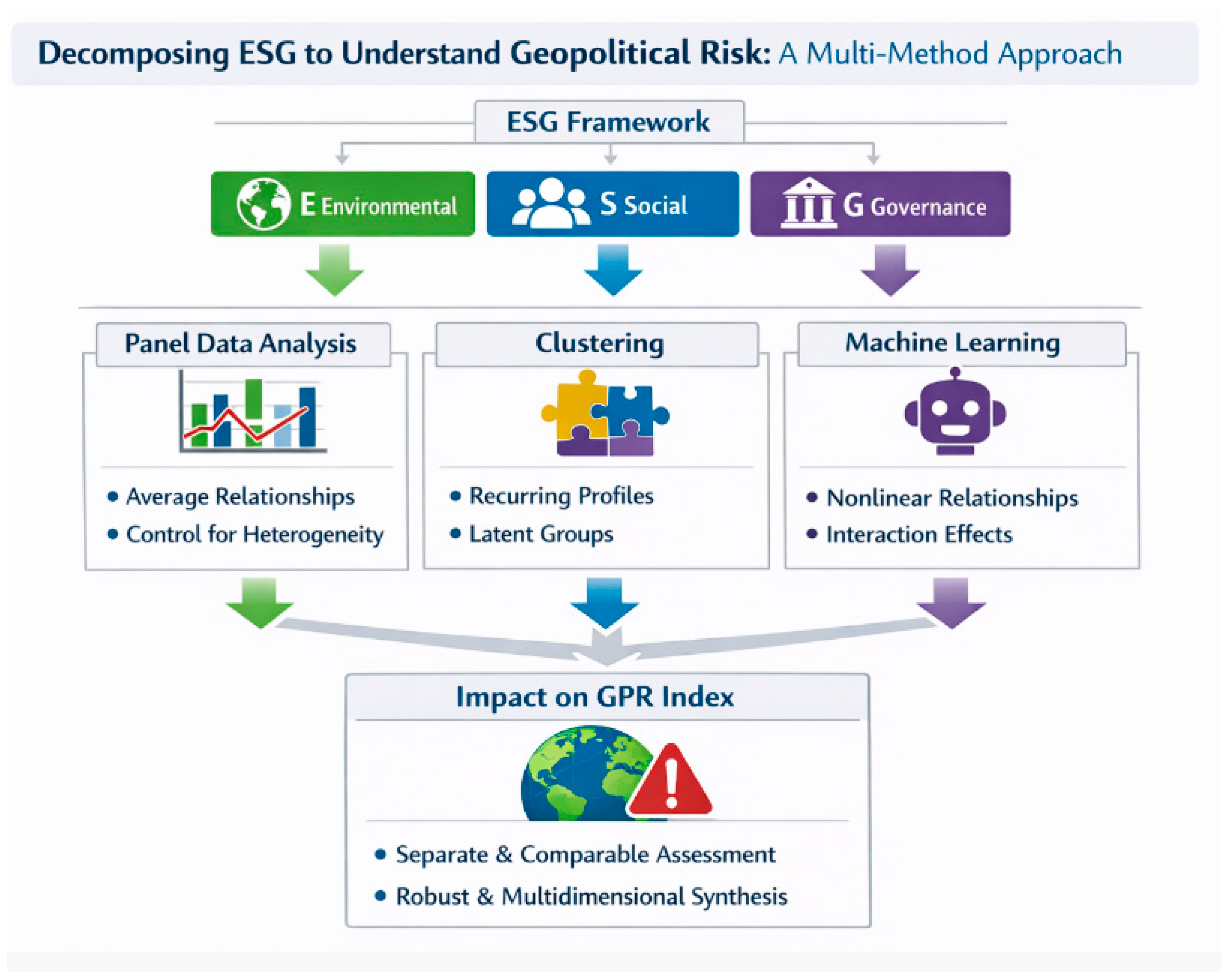
The research follows a methodological approach that clearly breaks down the ESG concept into its three pillars: Environmental (E), Social (S), and Governance (G). This helps examine the individual effects of these ESG aspects on geopolitical risk, as measured by the Geopolitical Risk (GPR) index introduced by Caldara and Iacoviello (2022). Instead of focusing on ESG as an aggregate measure, this analysis distinguishes among the three factors to enable an individual investigation of each. This is because it has been argued that environmental factors, societal factors, and governance factors affect the creation of geopolitical risk in different channels, to say nothing of their relative strength in this regard, especially in the context of structural changes like climate change (Bolton et al., 2020; Kahn et al., 2021). For each ESG factor, these three steps of the methodology are systematically followed. To begin with, panel econometric models are estimated to identify relationships over time and across countries, while accounting for unobserved heterogeneity. This makes it possible to identify statistically significant relationships that are interpretable from an economic theory perspective. This aligns with the empirical literature, which treats geopolitical risk as a measurable phenomenon that changes over time (Caldara & Iacoviello, 2022). Second, the application of clustering methods helps uncover the heterogeneity of the underlying structure and the presence of hidden group memberships of countries based on their ESG characteristics. Clustering allows the exploration of the interconnections among ESG variables, such as environmental vulnerability, social vulnerability, governance capacity, and levels of geopolitical risk. This approach aligns with the perception that systemic risks are driven not only by isolated shocks but also by the interconnections across several dimensions of sustainability (Bolton et al., 2020). Thirdly, machine learning regression techniques are used to capture nonlinear relationships and patterns that cannot be captured by econometric models. Such techniques are particularly useful in analyzing heterogeneous and nonlinear responses to environmental and climate-related variables in macroeconomic and political outcomes (Kahn et al., 2021). The approach combines panel data analysis, machine learning regression, and clustering techniques, each applied separately to each pillar of ESG factors, in a manner that compares results while leveraging their complementary advantages. In summary, this integrated framework for methodologies provides a holistic and robust evaluation of the individual and combined influences of Environmental, Social, and Governance variables on geopolitical risk, and goes beyond reduced forms to a more sustainability-focused perspective on geopolitical instability. See Figure 1.

Data Sources and Harmonization. The empirical analysis uses data from two main sources. Firstly, the Geopolitical Risk (GPR) index, as created by Caldara and Iacoviello, is publicly available in the official repository (https://www.matteoiacoviello.com, accessed on 23 October 2025). Originally released monthly, this index measures geopolitical risks by the proportion of newspaper articles on wars, geopolitical risks, and international conflicts. To use this index in the analysis, the monthly GPR index was aggregated to an annual frequency to match the ESG variables used. ESG-related variables were sourced from the World Bank ESG dataset (https://esgdata.worldbank.org, accessed on 23 October 2025), which provides internationally comparable ESG variables at the country level. No interpolation or extrapolation was performed on the data during harmonization. Data aggregation was performed for the GPR index, whereas the ESG variables were retained at their original annual frequency. A few observations in the dataset were missing and left as is to avoid introducing artificial data adjustments.

Clarifying the Direction of Analysis and the Limits of Causal Identification. The empirical specification used in this current analysis should not be interpreted as establishing strict causal identification within a structural econometric framework. The model does not employ instrumental variables, natural experiments, or quasi-experimental designs that aim to establish exogenous variation in ESG dimensions. Instead, the analysis tests the hypothesis that the Environmental, Social, and Governance dimensions act as structural conditioning factors that are systematically related to cross-country and intertemporal variations in geopolitical risks. Here, the ESG dimensions are conceptualized as foundational dimensions that affect a country’s exposure, sensitivity, and adaptive capacity to global disturbances. While a significant segment of the current literature treats geopolitical risks as exogenous shocks that condition ESG performance, particularly at the corporate/financial levels, this analysis adopts an alternative, converse analytical approach. It tests the hypothesis that sustainability fundamentals co-vary with and possibly influence the structural environment from which geopolitical risks emerge. As such, the analysis focuses on establishing patterned structural relationships rather than establishing causal directionality. As such, the findings should not be interpreted as establishing causal transmission channels between ESG fundamentals and geopolitical risks but rather as establishing conditional influence and embedded structural association between sustainability conditions and geopolitical risks. Within this framework, the panel structure of the dataset implicitly incorporates these common shocks and spillover channels. External disturbances are therefore indirectly embedded in the empirical design, as the model accounts for shared variance and correlated movements across countries. The evidence of cross-sectional dependence strengthens the interpretation of geopolitical risk as a globally networked process shaped by international interdependencies, rather than as a purely endogenous or country-specific political condition.

3.1. Theoretical Mechanisms Linking ESG Pillars to Geopolitical Risk

While the empirical strategy used here does not offer a structural identification of causality in a structural econometric model, the model is grounded in a theoretical structure that defines plausible channels of transmission between the pillars of Environmental, Social, and Governance (ESG) and geopolitical risks. The purpose of this subsection is not to establish claims of causal direction but to establish the structural channels through which the fundamentals of sustainability might affect exposure and vulnerability to geopolitical risks. The pillar of Environmental influences geopolitical risks mainly through channels related to resource scarcity, energy dependency, and climate risks. Nations that exhibit high energy dependency, water scarcity, environmental degradation, and climate risks might face economic stress, commodity-related economic volatility, and fiscal stress. These conditions might lead to high levels of domestic stress, dependency on volatile external sources, and vulnerability to global market disruptions. Environmental vulnerability might also trigger spillovers across borders through channels such as migration, inter-country resource conflicts, and energy security concerns. Hence, environmental vulnerability might act as a structural amplifier, affecting how external geopolitical shocks are absorbed and propagated. The Social Pillar operates through various mechanisms related to domestic cohesion, demographic dynamics, and distributive stability. High levels of inequality, poor healthcare and education facilities, a rigid labor market structure, and unmanaged migration rates are among the factors that may affect social stability within a nation-state. Therefore, if social cohesion within a nation-state is compromised, the likelihood of political polarization and institutional mistrust may increase. As a result, a nation-state’s ability to deal effectively with external shocks may diminish. In such a scenario, external disturbances, such as an energy crisis or international conflicts, may have a greater impact on the nation-state. The Governance Pillar acts as a moderating or filtering factor between various sustainability pressures or shocks and their potential impact on the nation-state. The quality of governance structures is a key determinant of how effectively a nation-state can address environmental or social sustainability pressures or shocks. It is a moderating factor that helps to manage the risks associated with external shocks or sustainability pressures. Therefore, a strong governance structure helps manage risks effectively by maintaining coordination across policies, enhancing crisis management capabilities, and minimizing uncertainty during periods of external stress. The combined effect of all these mechanisms suggests that ESG Pillars must be viewed as a group of interconnected structural conditioning factors rather than individual factors. Geopolitical risks are not created by individual political events; rather, they result from a combination of external disturbances or shocks and the structural sustainability that conditions the risks faced by a nation-state.

3.2. Boundary Conditions and Contextual Moderators of the ESG–Geopolitical Risk Relationship

The theoretical framework advanced in the current research also recognizes that the relationship between ESG dimensions and geopolitical risks is unlikely to be uniform. Instead, it is anticipated that the strength and direction of the relationship will be contingent upon boundary conditions that moderate the transmission channels. To begin with, the economic structure is seen as a critical boundary condition. In resource-dependent economies, particularly those with high reliance on fossil fuels or a commodity export base, the relationship between environmental stress and geopolitical risks may be more pronounced. This is because, in these economies, environmental stress, particularly that linked to climate change, might have a more significant macroeconomic and geopolitical impact, especially when it affects commodity markets. On the other hand, diversified economies with a more diversified production base might be more resilient and able to withstand environmental stress without it translating into geopolitical risks. The other boundary condition advanced in the current research is institutional capacity. The theoretical framework that has guided the current research recognizes that, despite levels of environmental or social stress, economies with high governance, particularly those with transparent institutions, robust regulatory systems, and independent judiciaries, may be able to mitigate the escalation into geopolitical risks. On the other hand, economies with low governance might be more susceptible to environmental or social stress, and instability might be more pronounced. Governance, therefore, plays a role as both a mechanism and a contextual moderator. Third, the development stage and demographic composition might also impact the results. In particular, the impact might be greater for developing economies undergoing rapid urbanization and/or demographic changes. On the contrary, the impact might be smaller for developed economies that enjoy high standards of public services and welfare systems, which could mitigate the destabilizing effects of similar pressures. Fourth, external integration and geopolitical positions also play a role in the ESG–risk nexus. In particular, countries that are highly integrated into the world economy might be more sensitive to external shocks, thereby amplifying the link between sustainability and geopolitical risks. At the same time, regional cooperation might act as a moderator of risk transmission. Therefore, the results obtained should be interpreted in the context of a conditional and context-dependent model. In particular, the relationship between ESG and geopolitical risks is not universal or deterministic. On the contrary, it follows the patterned structural relationships that vary depending on the economic structure, the quality of institutions, the development stage, and the degree of international integration. This, therefore, adds more theoretical content to the model while remaining consistent with the non-causal approach followed.

3.3. Integrated Multi-Method Analytical Strategy

The empirical methodology used here is specifically designed to be an integrated multi-method approach rather than a set of isolated techniques. Panel data analysis, clustering analysis, and machine learning techniques are used here as complementary analytical layers to address different yet related dimensions of the ESG-Geopolitical Risk nexus. To begin with, panel data analysis serves as the first layer of analysis. It estimates the average structural relationships between the pillars of Environmental, Social, and Governance dimensions and Geopolitical Risks across countries and over time. This methodology helps control for unobserved heterogeneity, time effects, and structural changes across countries and over time, thereby establishing structural patterns in the ESG-GPR nexus. It specifically operationalizes the key theoretical proposition that the fundamentals of sustainability act as structural conditioning factors. While this methodology is good at establishing average marginal effects, it is not very good at capturing nonlinear relationships and cross-country heterogeneity. Clustering analysis is introduced here to specifically address cross-country heterogeneity. Instead of relying on average structural relationships, clustering analysis focuses on structural regimes within the dataset. It identifies countries with similar ESG profiles and Geopolitical Risks. This methodology specifically helps observe heterogeneous architectures of sustainability and Geopolitical Risks across countries by empirically examining whether certain combinations of environmental risks, social risks, and good governance quality translate into specific types of Geopolitical Risks. This methodology provides a configurational view of the dataset that complements the variable-centered view provided by the panel data analysis methodology. It provides a structural view of country typologies that is consistent with the theoretical mechanisms established earlier. Third, it employs machine learning methods to expand the analysis’s scope by exploring nonlinear interactions among ESG variables. While panel models can capture linear relationships between variables and clustering can reveal structural regimes, machine learning approaches can uncover complex dependencies and nonlinear interactions between variables, which may not be feasible with traditional methods. This part of the analysis tests the nonlinear relationship between ESG variables and geopolitical risk, thereby corroborating the panel regression models’ findings. Thus, the three parts of the methodology can be considered interconnected and form an integrated whole. While panel regression establishes the baseline structural relationships between ESG variables and geopolitical risk, clustering reveals heterogeneous regime structures, and finally, machine learning approaches reveal nonlinear interaction effects. The consistency of findings across the different approaches provides additional triangulation, affirming the robustness of the theoretical arguments. Instead of being mutually exclusive, the approaches complement each other to create a multifaceted understanding of the relationships between ESG variables and geopolitical risk. The methodology is thus aligned with the theoretical framework of structural sustainability.

4. Environmental ESG Drivers of Geopolitical Risk: Evidence from Panel Models, Clustering, and Machine Learning

This section explores the link between the E dimension of ESG (Environment) and geopolitical risk, as measured by the Geopolitical Risk Index (GPR). The hypothesis is that, beyond being ecological outcomes, environmental conditions serve as structural risk drivers of instability, shaping climate risk, pollution, resource depletion, and energy structure, thereby influencing the magnitude of geopolitical risk, as captured by GPR. To test the link between the two, an empirical model is built that uses the set of E dimension variables to explain GPR values, using a panel of 42 countries from 2000 to 2023. The following subsections fulfill the above aim through three approaches: panel data, which estimates average effects of E dimension variables on GPR; clustering, which identifies groups of countries characterized by similar E dimension patterns, which are associated with varying levels of GPR; finally, machine learning regression, which explores nonlinear patterns of interaction between E dimension variables, which would not be captured through traditional regression models.

4.1. Panel Data Evidence on the Environmental (E) Dimension of ESG and Geopolitical Risk

To analyze the relationship between the E-Environment component of the ESG model and the GPR dimension, i.e., geopolitical risk, we estimated the following equation:

$$\begin{gathered} \mathrm{G}\mathrm{P}\mathrm{R}=\mathsf{\alpha }+{\mathsf{\beta }}_1{\left(\mathrm{N}\mathrm{R}\mathrm{D}\right)}_{\mathrm{i}\mathrm{t}}+{\mathsf{\beta }}_2{\left(\mathrm{E}\mathrm{C}\mathrm{O}\mathrm{A}\right)}_{\mathrm{i}\mathrm{t}}+{\mathsf{\beta }}_3{\left(\mathrm{C}\mathrm{H}4\right)}_{\mathrm{i}\mathrm{t}}+{\mathsf{\beta }}_4{\left(\mathrm{S}\mathrm{M}\mathrm{D}\mathrm{W}\right)}_{\mathrm{i}\mathrm{t}} \\ +{\mathsf{\beta }}_5{\left(\mathrm{R}\mathrm{E}\mathrm{N}\right)}_{\mathrm{i}\mathrm{t}}+{\mathsf{\beta }}_6{\left(\mathrm{T}\mathrm{C}\mathrm{L}\right)}_{\mathrm{i}\mathrm{t}} \end{gathered}$$

where $\mathrm{i}=42$ and $\mathrm{t}=[2000;2023]$.

Specifically, the variables analyzed are described in the following

Table 2. Environmental (E) Variables Used to Analyze the Impact of ESG on Geopolitical Risk.

	Variable	Full Name	Description
Y	GPR	Country GPR—Geo Political Risk	Index measuring a country’s geopolitical risk based on the percentage of news articles related to political tensions, conflicts, and instability.
X	NRD	Adjusted savings: natural resources depletion	Indicator of the reduction in natural capital due to the extraction of resources such as minerals, energy, and forests, expressed as a share of national income.
	ECOA	Electricity from coal	Share of total electricity generation produced from coal-fired power plants.
	CH4	Methane emissions	Amount of methane emissions generated by human activities such as agriculture, waste management, and energy production, a gas with high climate impact.
	SMDW	Safely managed drinking water	Percentage of the population with access to safely managed and continuously available drinking water services.
	REN	Renewable energy consumption	Share of total energy consumption derived from renewable energy sources.
	TCL	Tree Cover Loss	Area of forest cover lost over a given period, used as an indicator of deforestation and environmental degradation.

Note: The table reports the dependent variable and the set of environmental indicators representing the E pillar of ESG. These variables capture natural resource depletion, energy structure, emissions, ecosystem degradation, and access to essential environmental services relevant for explaining geopolitical risk.

.

For the analysis, the dependent variable is Geopolitical Risk (GPR), captured using the Caldara and Iacoviello (2022) index, which measures a country’s geopolitical risk by counting the number of news stories related to conflict, political tension, and institutional instability. This approach has enabled GPR to be treated as a time-varying, measurable macro-political phenomenon with significant economic effects (Caldara & Iacoviello, 2022; Caldara et al., 2020). The research will investigate how well the chosen factors explain differences in GPR levels for a panel data sample of 32 countries for 16–19-year-olds, yielding a total of 600 data points. This is consistent with the growing literature that focuses on the role of climate change, environmental degradation, and the structure of the energy system as sources of economic and political instability (Bolton et al., 2020; Kahn et al., 2021). Four different econometric models were estimated: Pooled OLS, Fixed Effects Model, Random Effects Model via GLS, and Weighted Least Squares. This allows for easy robustness checks under different assumptions regarding the nature of heterogeneity and country-specific structural differences. The Hausman test helped select between fixed- and random-effects models. It produced a p-value of 0.0086 and rejected the null hypothesis of consistency of the GLS estimator. This supported the fixed effects model. The fixed-effects model had an R-squared of 0.92 under the LSDV model. This suggests that GPR is driven mostly by country-specific variables. However, the R-squared of 0.14 under the fixed-effects model suggests low explanatory power for the variables. The coefficients are comparable under the different models. This suggests that the results are robust. Natural Resource Depletion: The coefficient is negative and significant in all models, suggesting that as natural resource depletion increases, geopolitical risk decreases. While this result might seem counterintuitive at first, it could be because resource-exploiting countries tend to adopt rent-based economies, which, in turn, might suppress political instability in the short run, as per political economy theories on resource rents and stability. The electricity from coal has a significantly positive coefficient, indicating that greater reliance on coal for electricity production is associated with higher GPR, suggesting vulnerability to systemic fragility. This implies that countries dependent on fossil fuels are vulnerable to global shocks, global decarbonization, and conflicts over energy resources (Bolton et al., 2020). Methane emissions are among the most significant factors, and they have a positive, highly significant coefficient in all models. An increase in methane emissions could also signal an unsustainable development trend, leading to social unrest, health issues, and climate change, all of which could heighten geopolitical risk. This could also be linked to the fact that environmental stress and emissions have been found to contribute to economic and political instability (Kahn et al., 2021; Miah et al., 2021). Safe Drinking Water also has a positive and significant coefficient. Care should be exercised in interpreting this result, since the availability of safe water is usually a proxy for development, though in some cases it may be related to rapid urbanization and population concentration, which, in institutionally weak environments, may produce a different type of inequality and conflict dynamics (Böhmelt et al., 2014). Results for Renewable Energy Consumption are mixed, as it is positive in the Random Effects, Fixed Effects, and Random & Fixed Effects models, but negative in the Pooled OLS and Weighted Least Squares models. This volatility could indicate endogeneity, as there may be a correlation between Renewable Energy Consumption and country-specific effects. In the more accurate models, the positive sign may indicate that the transition process, especially during the initial stages, is associated with transition costs that increase political uncertainty, as discussed by Bolton et al. (2020). Tree Cover Loss has a positive, significant coefficient, indicating that deforestation is positively associated with geopolitical risk. This is supported by the literature, which links environmental degradation, rural livelihoods, and land-use conflicts, especially in environments with low adaptive capacity (Burke et al., 2018). The fixed-effects model has strong explanatory power, but several econometric issues warrant note. The White test for heteroskedasticity and the Wald test both reject the null of homoskedastic residuals, suggesting heteroskedasticity across countries. The Pesaran CD tests indicate cross-section dependence, suggesting cross-country spillovers: shocks in one country can spill over into others. This may reflect global geopolitical risks in the energy markets (Pesaran & Tosetti, 2011). The Wooldridge test suggests the presence of first-order autocorrelation, while the tests for In sum, the analysis demonstrates that environmental and energy-related dynamics are crucial determinants of GPR. While the use of coal, methane emissions, and forest destruction are related to GPR, the relationship between GPR and the use of natural resources is much more complex and may be mediated by institutional and economic mechanisms. The relationship between the energy transition and GPR is not one-dimensional and may be contingent on various country-specific factors and adjustment costs. The findings of the analysis provide evidence that the role of environmental policy is not limited to its relationship with the environment, as the increasing relevance of environmental disasters to financial and geopolitical risk is well established in the literature, including the role of climate change in shaping global economic policy, including the prevention of global conflicts, as established in Caldara et al. (2020) and Pankratz et al. (2023). In addition, despite the econometric challenges posed by heteroscedasticity, cross-sectional dependence, and endogeneity, the analysis provides clear evidence that environmental sustainability is a structural determinant of GPR and should be mainstreamed into policymakers’ strategies to contribute to long-term GPR. See

Table 3. Environmental (E) Variables Used to Analyze the Impact of ESG on Geopolitical Risk.

Dependent Variable:	GPR
Time-series length	minimum 16, maximum 19
Cross-Sectional units	32
Observation	600
Models	Random-effects (GLS)			Fixed-effects			Pooled OLS			WLS
	Coefficient	Std. Error	z	Coefficient	Std. Error	t-ratio	Coefficient	Std. Error	t-ratio	Coefficient	Std. Error	t-ratio
const	−1.00 ***	0.20	−4.84	−1.30 ***	0.24	−5.41	−0.06 ***	0.08	−0.79	0.02	0.01	1.55
NRD	−0.008 **	0.004	−2.06	−0.009 **	0.004	−2.25	−0.01 **	0.006	−3.07	−0.007 ***	0.001	−4.28
ECOA	0.001 **	0.0007	2.04	0.001 **	0.0007	2.03	0.001 ***	0.0007	2.20	0.001 ***	0.0002	6.62
CH4	0.374 ***	0.04	7.74	0.45 ***	0.05	8.29	0.11 ***	0.03	3.00	0.04 ***	0.01	4.27
SMDW	0.007 ***	0.001	3.93	0.009 ***	0.002	3.91	0.002 ***	0.0007	3.81	0.001 ***	0.0001	6.99
REN	0.005 ***	0.001	3.68	0.007 ***	0.001	4.69	−0.007 ***	0.001	−7.01	−0.004 ***	0.0002	−14.91
TCL	3.11675 × 10−8 **	1.50640 × 10−8	2.06	3.13847 × 10−8 **	1.50946 × 10−8	2.07	1.02196 × 10−7 ***	2.65296 × 10−8	3.85	6.11747 × 10−8 ***	1.11685 × 10−8	5.47

Notes: Standard errors in parentheses. *** p < 0.01, ** p < 0.05.

.

Methodological Robustness and Identification Strategy. The econometric model explicitly addresses the methodological concerns raised by cross-sectional dependence, heteroskedasticity, serial correlation, and endogeneity between environmental, social, and governance (ESG) fundamentals and geopolitical risk (GPR). First, the diagnostic tests for the baseline model with fixed effects indicate robust evidence of cross-sectional dependence (Pesaran’s CD tests are significant at p < 0.001) and heteroskedasticity (White and Wald tests are rejected). This is consistent with the global and interconnected nature of geopolitical risk. To address second-generation panel data problems, the main results were re-estimated with fixed effects and were robust to the Driscoll–Kraay standard errors, which account for heteroskedasticity, serial correlation, and other forms of cross-sectional dependence. The results are consistent, especially for SMDW, CH₄, NRD, and REN, suggesting that the main results are unlikely to be driven by misspecified covariance structures. Secondly, serial correlation was identified by performing the Wooldridge test. The Driscoll–Kraay procedure directly addresses this issue by allowing for autocorrelation up to a specified lag structure. This minimizes bias in inference. The stability of the estimates provides further support for the robustness of the identified associations. Thirdly, endogeneity issues, particularly reverse causality between ESG conditions and GPR, were addressed by employing instrumental-variable panel-data estimators. ECOA, SMDW, and CH₄ were treated as endogenous variables and instrumented with macro-institutional variables such as GDP growth rates, control of corruption, inequality, life expectancy, unemployment rates, internet penetration rates, and population density. The FE-TSLS and RE-TSLS estimates corroborate the statistical significance of the ESG components. This supports the notion that reverse causality does not fully account for the identified associations. While addressing endogeneity issues with instrumental variables provides further assurance regarding the identified associations, we would like to emphasize that structural identification would benefit from the use of dynamic panel data models, particularly system GMM models, which represent an interesting future research direction. Overall, the findings from all three models reinforce the interpretation of the ESG pillars as structural conditioning factors for geopolitical risks rather than an artifact of model misspecification. See

Table 4. Comparison of Instrumental Variables (IV) Panel Estimation Models: FE-TSLS, RE-TSLS, and FE Driscoll–Kraay.

Variable	FE-TSLS	RE-TSLS (G2SLS)	FE (Driscoll–Kraay)
const	−3.08612 *** (0.780516)	−1.81298 *** (0.508133)	−0.944140 *** (0.333461)
ECOA	0.00651966 ** (0.00272257)	−0.000976706 (0.00274878)	—
SMDW	0.0314617 *** (0.00734710)	0.0182224 *** (0.00458437)	0.00853515 *** (0.00239437)
CH4	0.365362 ** (0.179757)	0.405722 *** (0.136278)	0.315042 ** (0.121230)
NRD	—	—	−0.00904700 ** (0.00369897)
REN	—	—	0.00427132 *** (0.00127094)
Endogenous	ECOA, SMDW, CH4	ECOA, SMDW, CH4	—
Instruments (Z)	GDPG, COR, GINI, LEX, UNEM, INT, PDEN	GDPG, COR, GINI, LEX, UNEM, INT, PDEN	—
Observations (N)	526	526	658
Model test	Wald χ2(3) = 22.469 (p = 0.0001)	Wald χ2(3) = 16.628 (p = 0.0008)	F(4, 31) = 4.1675 (p = 0.0081)
R2	0.049	0.063	Within R2 = 0.0858

Notes: Standard errors in parentheses. *** p < 0.01, ** p < 0.05. Driscoll–Kraay (HAC) standard errors are robust to heteroskedasticity, serial correlation, and cross-sectional dependence—indicates variable not included in that specification.

.

4.2. Environmental Risk Regimes and Geopolitical Risk: A Clustering-Based Assessment

The choice of the most appropriate clustering algorithm must be based on a balanced evaluation of several performance indicators, since each metric captures a different aspect of clustering quality (Arbelaitz et al., 2013). In this comparison, all indicators have been normalized so that higher values always correspond to better performance, allowing a coherent cross-algorithm assessment. Among these indicators, particular attention is devoted to the HH index, which measures concentration and balance in cluster sizes and is especially relevant when interpretability and representativeness of clusters are important. Hierarchical clustering clearly stands out in terms of internal cohesion and separation. It achieves the maximum normalized score for minimum separation, Pearson’s γ, Dunn index, and entropy, and also performs very well on the Calinski–Harabasz index. These results indicate that hierarchical clustering produces well-separated and compact clusters with high structural quality (Arbelaitz et al., 2013). However, its HH index is zero, indicating a very high concentration of observations in a small number of clusters. This severe imbalance reduces the practical usefulness of the solution, especially when the objective is to obtain clusters of comparable size or to avoid dominance by a few large groups. K-Means also shows excellent performance on some classical validity indices, particularly Pearson’s γ and the Calinski–Harabasz index, where it reaches the maximum normalized value. Nevertheless, its HH index is extremely low, indicating strong concentration and limited balance in cluster sizes. This makes K-Means less suitable in contexts where cluster size homogeneity is a priority. Density-based methods display the opposite profile. While they perform weakly on separation and compactness metrics, they achieve the maximum score on the HH index. This indicates a very balanced distribution of observations across clusters, which is a desirable property when the goal is to avoid overrepresentation and ensure interpretability; moreover, density-based clustering frameworks are explicitly designed to capture heterogeneous structures and distinguish clusters from noise (Campello et al., 2015). However, the poor performance on most quality indices suggests limited overall clustering structure. Random Forest–based clustering emerges as the most balanced solution. It does not dominate in any single metric, but it consistently performs well across all indicators and shows a high HH index, second only to the density-based approach. This implies a good compromise between cluster quality and size balance. More broadly, machine learning approaches are often preferred in applied settings when the underlying relationships are complex and potentially nonlinear, as they can enhance robustness and discriminative power across high-dimensional feature spaces (Martínez Torres et al., 2019). Considering all indicators jointly, and giving particular weight to the HH index, Random Forest appears to be the most appropriate algorithm, as it provides a robust trade-off between structural quality and balanced cluster composition. See

Table 5. Environmental (E) Variables Used to Analyze the Impact of ESG on Geopolitical Risk.

Metric	Density Based	Fuzzy C-Means	Hierarchical	Model Based	K-Means	Random Forest
Maximum diameter	0.326	0.500	1.000	0.000	0.837	0.674
Minimum separation	0.161	0.000	1.000	0.665	0.238	0.558
Pearson’s γ	0.103	0.017	1.000	0.000	1.000	0.140
Dunn index	0.095	0.000	1.000	0.471	0.232	0.494
Entropy	0.000	0.822	1.000	0.997	0.943	0.601
Calinski–Harabasz index	0.653	0.000	0.816	0.001	1.000	0.509
HH-Index	1.000	0.585	0.000	0.219	0.055	0.743

Note: The table reports the dependent variable and the set of environmental indicators representing the E pillar of ESG. These variables capture natural resource depletion, energy structure, emissions, ecosystem degradation, and access to essential environmental services relevant for explaining geopolitical risk.

.

This study aims to determine the contribution of Environmental dimension variables to ESG ratings in explaining geopolitical risks, as represented by the Geopolitical Risk (GPR) Index. The segregation of countries into clusters based on an extensive database covering environmental issues, energy sources, climate change, and natural resource depletion enables the identification of environmental trends correlated with different levels of geopolitical risk. In this study, Geopolitical Risk is considered to be affected by environmental issues rather than being solely a political construct. It should be noted that geopolitical risks are influenced by environmental issues, in line with the argument that “climate shocks are viewed as systemic risk multipliers” (Bolton et al., 2020; Kahn et al., 2021). The clusters with higher levels of Geopolitical Risk (e.g., clusters 1, 3, 5, 6, and 7) generally indicate adverse environmental trends, including high levels of CO₂ and methane emissions and the use of fossil fuels or coal-based energy production. In some instances, it has also been found to be associated with high Cooling Degree Days, Heat Index, or energy intensity, which may be considered to be indicative of high levels of climate change or stress. This may align with the argument that “Environmental Degradation and Climate Stress are associated with geopolitical risks through their ability to drive up costs, tensions, and reliance upon imported energy supplies” (Bolton et al., 2020; Kahn et al., 2021). Moreover, it may be argued that energy or environmental issues are linked to economic or political issues (Şahin & Chen, 2023). In addition to environmental issues, resource depletion trends may also have played a role in differentiating between clusters; losses in adjusted savings due to resource or forest depletion have been found to be generally higher in clusters with higher levels of Geopolitical Risk. Likewise, Tree Cover Loss and forest cover changes are usually higher in clusters with higher geopolitical risk levels, as increased land degradation or deforestation can increase competition for natural resources and livelihoods (Burke et al., 2018). However, a lower probability of staying in less favorable environments is associated with lower or negative GPR values (e.g., countries 2 and 8). These countries have favorable performances in terms of access to clean fuels and electricity, lower emissions intensity, and a higher share of renewable energy consumption/output, in addition to lower pollution levels (e.g., PM2.5) and stronger performances in terms of water use indicators such as access to safely managed drinking water service and sanitation service. In terms of ESG factors, stronger environmental sustainability is associated with a lower probability of geopolitical risk (Bolton et al., 2020). Climate variability indicators also support the above analysis; regions that experience higher water stress, higher freshwater abstraction rates, and SPEI values are associated with higher levels of GPR. Water scarcity and climate conditions act as risk multipliers, increasing competition for resources and the likelihood of conflict, both within and between nations. The presence of these regions in higher levels of GPR substantiates the relevance of environmental factors in geopolitical events, as emphasized in the literature on the relationship between conflict, cooperation, and water (Böhmelt et al., 2014). In particular, the energy structure appears as a highly significant channel: clusters with high dependence on fossil fuels, coal-based electricity, and energy imports show higher levels of GPR, while greater dependence on renewable energy is associated with lower geopolitical risks. This assertion resonates with the ESG framework, in which the Environmental pillar prioritizes the energy transition and its significance in mitigating and adapting to climate change, addressing global shocks, and managing geopolitical tensions (Bolton et al., 2020; Şahin & Chen, 2023). In conclusion, cluster analysis has confirmed that ESG’s Environmental factor has a strong relationship with GPR. Therefore, it has been identified that nations under considerable environmental pressure due to inefficient energy resources and vulnerability to climate change have a high propensity for GPR. On the other hand, nations making considerable progress in environmental performance, efficient resource management, and energy transition have lower geopolitical risks. The study has emphasized the strategic importance of environmental sustainability for GPR and has supported integrating environmental factors as explanatory variables in the GPR model (Kahn et al., 2021). See

Table 6. Environmental Clusters and Geopolitical Risk (GPR): Cluster-Level Standardized Environmental Indicators.

	GPR	ACF	ELEC	NRD	NFD	AGL	AFF	WAT	CO2	CDD	ECOA	ENI	EINT	ENU
Cluster 1	0.384	−0.701	0.760	−0.667	−0.009	0.476	0.014	−0.412	0.346	0.284	0.470	−0.666	−0.093	0.705
Cluster 2	−0.503	0.800	−0.465	1.725	0.502	−0.961	−0.522	−0.351	−0.744	−0.487	−1.008	1.133	0.027	−0.455
Cluster 3	0.384	−0.535	−1.545	−0.806	0.261	0.721	−0.717	0.648	0.346	−1.164	1.591	0.897	−1.323	−0.356
Cluster 4	0.272	0.306	0.622	−0.564	−0.504	−0.342	0.865	0.703	0.241	0.327	−0.484	−0.706	0.215	−0.405
Cluster 5	0.384	−0.556	−0.589	0.800	−0.122	0.423	1.693	−0.507	0.346	0.570	−0.300	−1.528	1.440	0.429
Cluster 6	0.384	−0.395	0.499	−0.270	−0.288	−0.219	−0.193	−0.730	0.346	0.567	−0.374	−0.104	0.288	−0.333
Cluster 7	0.384	−0.545	−1.061	−0.199	−1.081	0.874	0.663	0.419	0.346	0.598	0.492	1.596	0.606	0.137
Cluster 8	−1.677	1.649	0.537	1.409	−0.403	−1.159	−0.208	−0.370	−1.112	0.045	−1.258	−0.513	0.160	−0.422
Cluster 9	0.356	0.028	−1.196	−0.738	3.784	1.165	−0.296	2.447	−0.109	−0.643	0.778	0.695	0.960	1.095
	FOR	FOS	HI35	HDD	LST	WSTR	CH4	N2O	SMDW	SMSS	PM25	REN	SPEI	TCL
Cluster 1	0.226	−0.322	−0.296	0.304	−0.192	−0.540	−0.508	−0.447	0.612	0.778	−0.011	−0.185	0.035	0.070
Cluster 2	−1.213	0.030	1.054	−0.079	1.289	1.154	0.611	0.568	−0.720	−1.398	−0.325	0.621	−0.693	−0.851
Cluster 3	1.548	−0.350	−1.626	1.560	−0.197	0.071	−1.365	1.449	0.633	0.398	0.622	0.261	−0.673	−0.793
Cluster 4	0.222	−0.350	−0.104	0.065	−0.197	−0.017	0.792	−0.309	0.115	0.020	−0.286	−0.380	0.187	−0.351
Cluster 5	−1.027	−0.214	1.569	−0.742	−0.197	−0.622	0.971	−0.844	0.679	0.515	−0.473	−0.441	4.004	3.111
Cluster 6	−0.414	−0.349	0.471	−0.541	−0.164	−0.635	−0.323	−0.104	0.479	0.187	−0.330	−0.391	−0.073	0.169
Cluster 7	−0.040	−0.143	−0.194	−1.152	−0.197	−0.652	0.358	−0.992	0.588	0.865	0.265	−0.414	0.138	1.234
Cluster 8	−1.149	1.853	1.261	−0.926	−0.115	0.367	0.970	0.237	−2.006	−1.202	0.113	−0.323	0.232	0.489
Cluster 9	2.375	−0.348	−2.065	−0.376	−0.197	2.147	−0.295	−1.005	−0.744	−0.789	0.400	3.221	−0.683	−0.822

Note: Countries under strong environmental pressure, inefficient energy use, and high climate vulnerability exhibit higher GPR, while environmental sustainability, efficient resource management, and progress in clean energy transition reduce geopolitical risk.

.

This analysis uses the Environmental, Social, and Governance (ESG) approach, focusing specifically on the role of the Environmental (E) aspect in relation to geopolitical risk as defined by the Geopolitical Risk (GPR) index. The importance of the individual environmental variables in explaining the GPR index can be understood from the mean decrease in Gini importance, which highlights their role rather than focusing on the direct relationships among the variables. The most important variables in explaining the GPR index are climate and temperature variables: Heating Degree Days (HDD), Land Surface Temperature (LST), Cooling Degree Days (CDD), and Energy Use per capita (ENU) rank among the highest. The results of the analysis imply the importance of the vulnerability of the environment to climate and temperature factors in the explanation of the GPR index, suggesting the vulnerability of the regions to climate and temperature factors, which are also characterized by increased requirements for energy in terms of heating and cooling, indicating increased structural pressures in terms of the infrastructure, financial, and energy sectors of the regions, which can be reflected in increased geopolitical risk vulnerability. The results of the analysis, from the ESG aspect, imply the importance of climate vulnerability in the explanation of political risk, which suggests a direct link to political risk factors, indicating the importance of climate vulnerability in the explanation of political risk factors, which support the idea of the role of weather and climate factors in the explanation of economic and social risk factors (Dong & Tremblay, 2021; Carleton & Hsiang, 2016). Energy-related factors also appear prominently. Energy imports (ENI), energy intensity (EINT), electricity from coal (ECOA), fossil fuel consumption (FOS), and renewable energy consumption (REN) appear prominently. This helps reinforce the idea that energy systems and their efficiencies serve as basic channels for translating environmental performance into geopolitical risk. High levels of energy imports and fossil fuel use increase vulnerability to global risks, while inefficient energy use adds to environmental pressures. The prominence of renewable energy factors suggests that the energy transition has become increasingly important for both environmental impacts and geopolitics, in line with strategic-political economy approaches to climate/green transformation (Saidin & O’Neill, 2022). Depletion and land-use indicators: natural resource depletion (NRD), tree cover loss (TCL), forest area (FOR), and agricultural land (AGL) are also highly ranked. This is evidence that unsustainable use of natural capital can weaken resilience and heighten geopolitical risk through increased competition for land, food, and ecological services. The weight for agriculture, forestry, and fishing value added (AFF) underscores the importance of resource-based economic systems for resilience to environmental and geopolitical shocks, as evidenced by relationships between environmental pressure, biocapacity, and economic resilience (Nathaniel, 2021). The water-related indicators are integral to this framework and include annual water withdrawal (WAT), water stress (WSTR), safely managed drinking water (SMDW), sanitation (SMSS), and water quality (WQG). The importance of water scarcity and mismanagement as risk multipliers and potential causes of social unrest, international conflict, and instability underscores their relevance to GPR and supports the hypothesis that water security and sustainability are inextricably intertwined and carry direct geopolitical significance in regions prone to climate change and governance instability. Indicators of pollution and emissions, such as CO₂, CH₄, N₂O, and PM2.5, also carry significant weight in this context. These variables address not only climate change externalities but also environmental damage that may affect health, efficiency, and social and economic stability. This significance further underscores that not only climate change but also overall environmental degradation are components of geopolitical risk in various ways. Overall, the feature importances provide strong empirical support for the relevance of the Environmental pillar of ESG in explaining geopolitical risk. GPR is clearly associated with climate change, the structure of the energy system, resource depletion, water scarcity, and overall pollution. The fact that some variables have a less strong explanatory power does not mean that they are irrelevant, but that they could be drivers of GPR along paths and processes that are difficult to distinguish from the paths and processes for other types of risk, at least in the short term, while they could be distinguished over the medium and longer term. What the study clearly shows, however, is that considering environmental factors and sustainability issues is essential for understanding geopolitical risk as a whole. The Environmental pillar of ESG clearly represents a key element in explaining GPR and confirms the idea that climate change, resource management, the energy transition, and, more generally, environmental issues form the foundation for building geopolitical resilience and stability. See

Table 7. Feature Importance for Explaining the Geopolitical Risk (GPR) Index: Mean Decrease in Gini.

Feature Importance	Mean Decrease in Gini Index	Feature Importance	Mean Decrease in Gini Index
HDD	38.579	ENI	20.409
LST	35.864	NRD	18.926
ENU	33.333	TCL	18.739
CDD	30.943	REN	18.035
SMDW	27.971	CH4	17.672
WAT	26.039	PM25	16.723
AFF	25.857	N2O	15.744
CO2	25.358	FOS	15.436
WSTR	24.620	EINT	13.549
AGL	24.450	ELEC	13.399
SMSS	24.095	HI35	11.669
FOR	22.500	ECOA	11.394
ACF	20.975	GPR	9.214
SPEI	3.726	NFD	5.262

Note: The table reports feature importance based on the mean decrease in the Gini index from the machine-learning model. Higher values indicate greater explanatory power in predicting the GPR index, highlighting the relative relevance of environmental, energy, and climate-related variables.

.

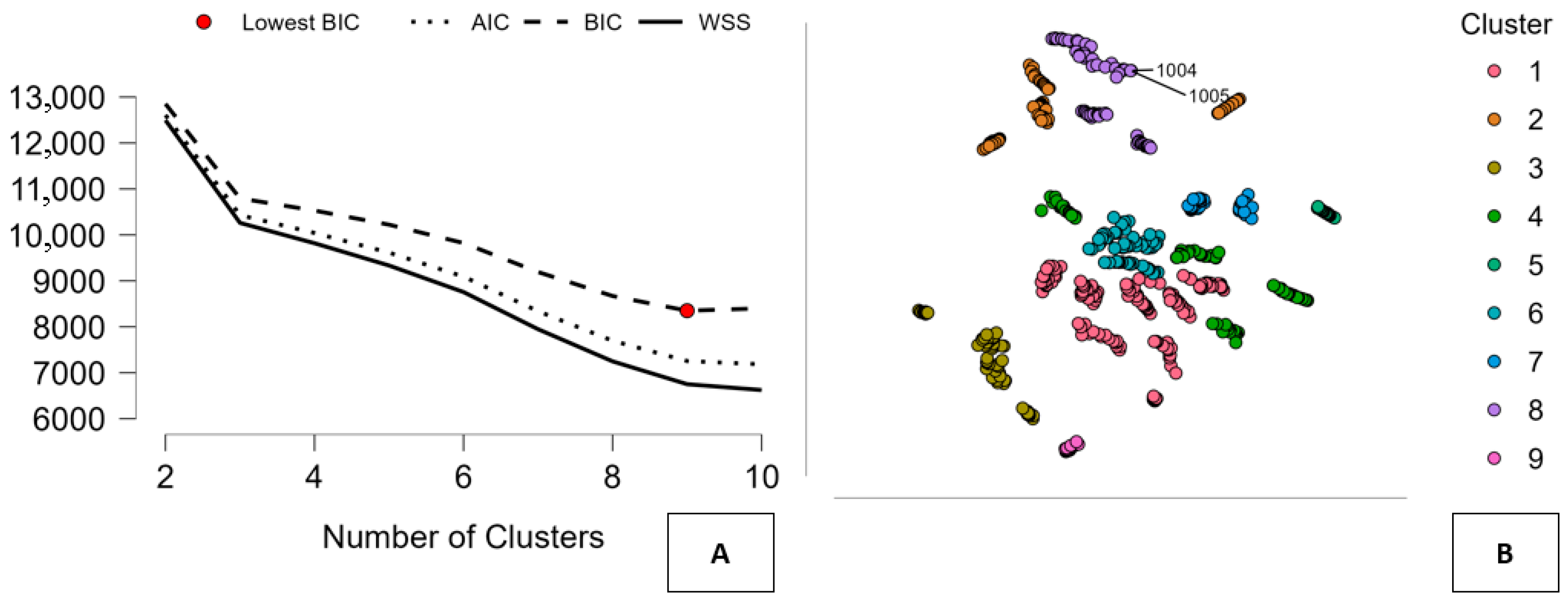
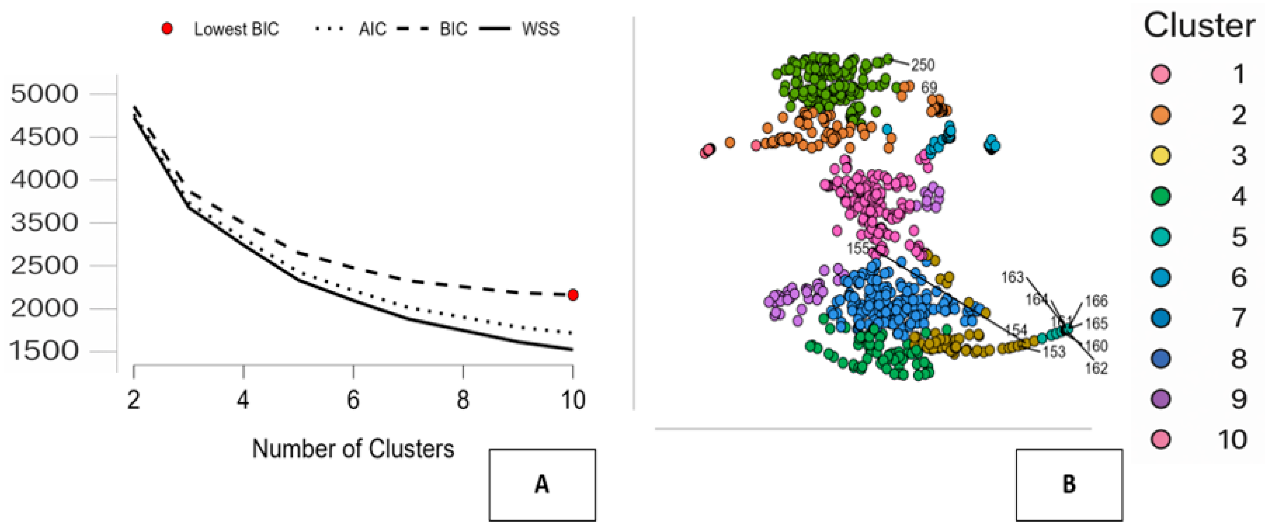
Interpretation and Limitations of Gini-Based Feature Importance. The results of the Random Forest analysis underscore the impact of climate-related variables on the variance in geopolitical risk. In particular, the feature importance scores based on the Mean Decrease in Impurity (MDI) measure indicate that adding environmental stress variables significantly improves the model’s performance. Although these results reaffirm the structural role of climate dynamics in the ESG/geopolitical risk relationship, interpreting the Gini-based feature importance scores should be done with caution. First, the MDI-based feature importance scores are biased toward variables with higher variance or more possible split points. Second, the presence of correlations between the features, which might be the case with the environmental and governance indicators, might lead to the shared importance of the variables across the features. Third, the Gini-based feature importance scores indicate the relative contribution of each feature to the ensemble estimator’s prediction. It should be noted that the Gini-based scores do not indicate the relative contribution to the identification of the underlying relationships. The following shows the results of the Random Forest-based clustering technique on the Environment (E) dimension of ESG, which help understand the impact of ESG on geopolitical risk (GPR). In panel A, the model selection step is depicted, which helps determine the appropriate number of clusters. The graph of the Within-Cluster Sum of Squares (WSS) measure, together with the information criteria AIC and BIC, decreases as the number of clusters increases, thereby indicating an improvement in the model’s fit. However, the BIC graph reaches a minimum at approximately 9 clusters, marked with a red circle. This result helps derive an appropriate balance between model fit, as captured by the model’s explanatory power, and model simplicity, thereby suggesting that nine clusters are sufficient to adequately characterize the underlying data structure without falling prey to model complexity. The strategy of using multiple internal criteria to validate clusters is consistent with the clustering literature, which suggests an appropriate balance between compactness, separation, and simplicity of clusters to adequately characterize the underlying patterns of multidimensional data (Arbelaitz et al., 2013). Panel B above shows a two-dimensional representation of this clustering outcome. Each data point in this graph represents an observation described by a variety of environmental factors, which are grouped by their cluster identities, indicated by different colors. This shows that countries have been effectively grouped or partitioned based on their environmental characteristics using the Random Forest method, indicating that this method can handle a variety of nonlinear relationships in a dataset (Martínez Torres et al., 2019). These groups or regimes represent different factors, such as climate vulnerability, energy systems, resource use, and environmental distress, that fall under the Environmental pillar of ESG analysis. In general, the use of sophisticated machine learning algorithms for representation learning and pattern extraction provides a more complex description of environmental regimes than traditional linear approaches (Ismail Fawaz et al., 2019). The identification of distinct environmental profiles associated with varying degrees of GPR helps interpret the concept of geopolitical risk as an effect driven by environmental sustainability, climate-related stress, and energy dependence. This further emphasizes the importance of the Environmental dimension in the ESG framework analysis of geopolitical risk. See Figure 2.

Environmental Dimension and Geopolitical Risk. The results from environmental clustering indicate a strong relationship between geopolitical risk and the configurations of structural climate and energy risks. In particular, countries that display high dependence on fossil fuels, high emissions intensity, high water stress, and high exposure to climate risk are found to be located in high global geopolitical risk (GPR) regimes. In turn, countries that exhibit high levels of renewable energy penetration, low pollution intensity, and high resource efficiency face much lower geopolitical risk. Hence, the Environmental pillar appears to act primarily through external channels of vulnerability, with environmental degradation and energy dependence increasing geopolitical risk, while sustainability transitions and climate risk reducing it.

4.3. Machine Learning Prediction of Geopolitical Risk from Environmental ESG Indicators: Model Comparison and Key Drivers

Based on the normalized results (on a scale from 0 to 1, with higher values indicating better performance), the KNN model is the best-performing. The objective evidence clearly reveals that for all the tested parameters, such as MSE, scaled MSE, RMSE, MAE/MAD, MAPE, and R², the best possible result of 1.00 has been achieved by the KNN model. It is clear that the model has achieved the minimum possible error and the maximum possible goodness of fit. Moreover, it can also be concluded that there is no trade-off between accuracy and goodness of fit because the minimum error is achieved at the highest value of R². The second-best algorithm here is the Random Forest algorithm. The algorithm’s performance is consistent across all metrics, particularly MSE, RMSE, and R², where it comes very close to the best results achieved by the KNN algorithm. It does not achieve the highest score across all aspects, indicating slightly lower accuracy than the KNN algorithm, though its robustness is very high. Linear Regression and Regularized Linear Models give intermediate results. They display good interpretability but moderate error, which is clearly inferior to the performance of KNN and Random Forest Algorithms, but could be useful if interpretability is of primary importance. Boosting, Decision Tree, and SVM have relatively weaker performances. Specifically, the Decision Tree has close to zero scores for some metrics, indicating that the model lacks the ability to generalize, whereas the SVM model has relatively low scores across most metrics, especially in overall fit. In conclusion, KNN is the best method for predictive accuracy, and Random Forest is a good alternative if robustness and generalization are the main priorities. See

Table 8. Comparative Performance of Machine-Learning Algorithms for Predicting the Geopolitical Risk (GPR) Index.

Metric	Boosting	Decision Tree	KNN	Linear Regression	Random Forest	Regularized Linear	SVM
MSE	0.35	0.00	1.00	0.58	0.96	0.60	0.53
MSE (scaled)	0.51	0.00	1.00	0.68	0.99	0.66	0.24
RMSE	0.25	0.00	1.00	0.45	0.92	0.47	0.40
MAE/MAD	0.14	0.25	1.00	0.12	0.85	0.00	0.23
MAPE	0.36	0.86	1.00	0.18	0.75	0.00	0.30
R2	0.43	0.00	1.00	0.64	0.98	0.61	0.22

Note: The table compares predictive performance across several algorithms using error and goodness-of-fit metrics. KNN achieves the highest overall accuracy, while Random Forest emerges as the second-best method, showing consistently strong performance and high robustness across metrics. Linear and regularized regression models provide intermediate results with greater interpretability but higher errors. Boosting, Decision Tree, and SVM display weaker performance, with the Decision Tree showing limited generalization ability.

.

The results are clear about how various factors contribute to explaining geopolitical risk (GPR) in the ESG model. The emphasis here is on how the KNN model can identify the actual roles of various environmental stressors in explaining geopolitical risk, rather than a linear model-based evaluation of variable importance. The most important variable is annual freshwater withdrawal (WAT), which shows the highest dropout loss in the model. The emphasis on freshwater withdrawal is a clear indicator of how geopolitical risk relates to water availability, and of how a lack of sufficient freshwater can contribute to geopolitical instability in regions where access to it is limited. Water scarcity is a key determinant in explaining geopolitical instability in regions where access to sufficient freshwater is limited (Böhmelt et al., 2014). Variables related to water infrastructure, such as safely managed sanitation service supply (SMSS) and safely managed drinking water service supply (SMDW), are also considered highly important. Similarly, variables related to pollution are considered highly important. Nitrous oxide (N₂O) emissions, fossil fuels (FOS), CO₂ emissions, methane (CH₄) emissions, and pollution related to PM2.5 are seen to have a high level of importance in explaining geopolitical risk in relation to changes in polluting production structures and types of fuels that are sensitive to international climate policy pressures and related adaptation costs in terms of social instability in relation to damage to the environment (Kahn et al., 2021; Şahin & Chen, 2023). Land use/Environmental Degradation also features prominently in the findings. The importance of Tree Cover Loss (TCL), Agricultural Land (AGL), Forest Area (FOR), as well as the value added by Agriculture, Forestry, and Fishing (AFF), is quite high, underscoring the role of unsustainable land use patterns and the reliance on resource-intensive sectors in the determination of geopolitical risk. These factors have been linked to food security risks, subsistence living, and resource-use conflicts, as underscored in research on agricultural ecology and environmental degradation (Chowdhury et al., 2022). Another notable category in the findings concerns the structure of the energy sector, which features prominently in the KNN findings. Renewable Energy Use (REN), Energy Intensity (EINT), Electricity Generated from Coal (ECOA), Energy Use per Capita (ENU), as well as Energy Imports (ENI), all indicate significant importance in the determination of geopolitical risk, underscoring the role of energy generation as well as consumption in the determination of geopolitical risk. The importance of renewables also underscores the significance of the energy transition in geopolitics, especially amid systemic change in the energy sector (Şahin & Chen, 2023). The role of SPEI, Heat Index 35 (HI35), HDD, CDD, and Land Surface Temperature (LST) is significant in determining geopolitical risk, highlighting the impact of climatic risks as shown in research on extreme climatic events and geopolitics (Kahn et al., 2021). Findings strongly affirm the role of the Environmental factor in determining geopolitical risk, underscoring the influence of water stress, emissions, and climatic risks on ESG risk management. The role of the environment in determining geopolitical risk also underscores the importance of environmental sustainability in geopolitical risk management, underscoring sustainability’s role in geopolitics as a phenomenon that extends well beyond the ecological sphere into the realm of risk management. See

Table 9. Environmental Feature Importance from the KNN Model Based on Mean Dropout Loss.

Feature Importance Metrics	Mean Dropout Loss	Feature Importance Metrics	Mean Dropout Loss
WAT	0.190	WSTR	0.083
N2O	0.165	SMSS	0.082
FOS	0.110	NRD	0.081
SPEI	0.109	NFD	0.079
TCL	0.109	ENU	0.079
REN	0.099	HI35	0.078
EINT	0.097	SMDW	0.075
ECOA	0.095	ACF	0.075
AFF	0.092	ELEC	0.074
AGL	0.092	HDD	0.074
PM25	0.088	ENI	0.074
CO2	0.087	LST	0.074
CH4	0.085	CDD	0.074
FOR	0.084

Note: The table reports environmental feature importance derived from the KNN model using mean dropout loss. Emissions, land degradation, energy structure, and climate-related risks emerge as key components of the Environmental pillar of ESG, highlighting environmental sustainability as a core determinant of geopolitical risk rather than a purely ecological concern.

.

As shown in the above table, a local explanation for the GPR model’s predictions based on the KNN model is available, with particular emphasis on the Environmental (E) component of the ESG model. In all five cases, a predicted GPR value is juxtaposed with a baseline value, and individual factors help explain how geopolitical risk is reduced relative to the baseline. While in all five cases the predicted GPR remains below the baseline value of 0.224, this is consistent with an understanding of geopolitical risk as a measurable and dynamic process subject to a range of structural factors but not political factors in the short term (Caldara & Iacoviello, 2022). However, the reduction in geopolitical risk is seen to result from a range of factors within the environmental dimension, rather than a single dimension. Within the energy dimension itself, energy structure and utilization are particularly important in this regard. For instance, factors such as electricity from coal (ECOA), fossil fuels (FOS), and energy use per capita (ENU) frequently contribute negatively across a range of different scenarios, particularly in relation to scenarios 1, 2, and 5. This suggests that lower coal use and a moderate overall energy use are associated with lower geopolitical risk. This is consistent with an ESG perspective that energy systems play a critical role in reducing geopolitical risk (Bolton et al., 2020). Similarly, renewable energy use (REN) often contributes positively across a range of scenarios, particularly in relation to scenario 1. This suggests that a cleaner form of energy is associated with geopolitical stability and is consistent with a range of evidence on climate transition, risk reduction, and resilience building (Pankratz et al., 2023). Water-related channels form another important category. The annual water withdrawal (WAT) and water stress (WSTR) indicators have negative weights, indicating that lower water pressure is associated with lower GPR. However, higher water withdrawal, as in case 5, has a positive effect on GPR, supporting the argument for the role of water scarcity and pressure in the environment as an important risk multiplier. This argument finds support in the literature on the role of water availability and related indicators in political instability and conflict across various parts of the world (Böhmelt et al., 2014). The indicators of emissions and pollution also support the argument of systemic impacts on GPR. Methane emissions (CH₄) have a negative effect on GPR, suggesting lower geopolitical risk in environments with methane. The effect of nitrous oxide (N₂O) emissions on GPR, however, is positive. The effect of carbon dioxide (CO₂) on GPR, though small, is positive, suggesting higher geopolitical risk in environments with higher CO₂ emissions. The effect of particulate matter (PM2.5) on GPR is unclear; it can sometimes have a positive effect, underscoring the role of environmental degradation in the stability of political regimes and its implications for geopolitical risk. This argument finds support in the literature on the macroeconomic and political impacts of climate change and its externalities, which impose systemic costs on the macroeconomy and increase geopolitical risk (Kahn et al., 2021). Land use and ecosystem variables also shape these predictions. Agricultural land (AGL), forest area (FOR), and tree cover loss (TCL) are consistently negative, suggesting better land management helps reduce geopolitical risk. Climate stress variables such as Cooling Degree Days (CDD), Heating Degree Days (HDD), Land Surface Temperature (LST), and Heat Index (HI35) are always present but are smaller contributors, supporting their role as background factors in geopolitical risk (Kahn et al., 2021). As such, these results reinforce the overarching theme presented by the ESG results: that GPR is significantly affected by environmental conditions. Water security, energy type and emissions, land use, and climate variables collectively determine whether a country’s environment exacerbates or reduces GPR. The fact that each of these five cases has a predicted GPR well below the baseline reinforces the argument that environmental upgrades are a net positive contributor to geopolitical risk and that environmental sustainability is a structural component of GPR as part of a larger risk and resilience model (Bolton et al., 2020; Pankratz et al., 2023). See

Table 10. Local Environmental Contributions to Predicted Geopolitical Risk (GPR) Across Five Cases.

Case	Predicted	Base	ACF	ELEC	NRD	NFD	AGL	AFF	WAT	CO2	CDD	ECOA	ENI	EINT
1	0.115	0.224	0.003	0.003	0.006	4.247 × 10−4	−0.036	0.002	8.904 × 10−4	0.004	3.699 × 10−4	−0.062	0.001	0.004
2	0.085	0.224	−8.767 × 10−4	0.004	0.008	4.110 × 10−5	−0.033	−0.003	−0.011	0.003	0.002	−0.003	2.055 × 10−4	−0.017
3	0.190	0.224	0.002	0.003	0.006	0.001	−0.004	−0.002	−0.012	0.004	0.007	−0.008	5.479 × 10−4	0.008
4	0.190	0.224	0.002	0.003	0.008	4.521 × 10−4	−0.012	0.003	0.011	−0.001	0.009	−0.028	0.001	0.009
5	0.185	0.224	0.002	0.005	7.123 × 10−4	0.001	0.010	3.288 × 10−4	0.025	0.003	0.005	−0.070	0.002	0.024
ENU	FOR	FOS	HI35	HDD	LST	WSTR	CH4	N2O	SMDW	SMSS	PM25	REN	SPEI	TCL
−0.008	−0.004	−0.009	−0.001	1.096 × 10−4	−0.005	−0.031	−0.019	0.017	3.151 × 10−4	0.008	−0.009	0.041	−0.009	−0.006
−0.027	−0.006	−0.011	−0.002	−1.096 × 10−4	0.004	−5.479 × 10−5	−0.067	0.017	−6.164 × 10−4	0.002	7.808 × 10−4	0.018	−0.010	−0.007
−0.020	−0.005	0.001	1.507 × 10−4	0.009	0.013	−0.022	−0.060	0.019	−0.002	0.005	0.023	0.004	0.001	−0.008
−0.008	0.013	−0.019	−1.644 × 10−4	0.012	−0.003	−0.038	−0.051	0.019	−0.004	0.008	0.039	0.000	0.002	−0.008
0.011	0.006	−0.029	−9.589 × 10−5	0.002	0.004	−0.008	−0.075	0.019	−9.315 × 10−4	0.002	0.011	−0.001	0.022	−0.011

Note: Geopolitical risk is shaped by environmental conditions: water security, energy mix, emissions, land use, and climate. In all five cases, predicted GPR falls below baseline, underscoring environmental sustainability as a structural stabilizer of geopolitical risk.

.

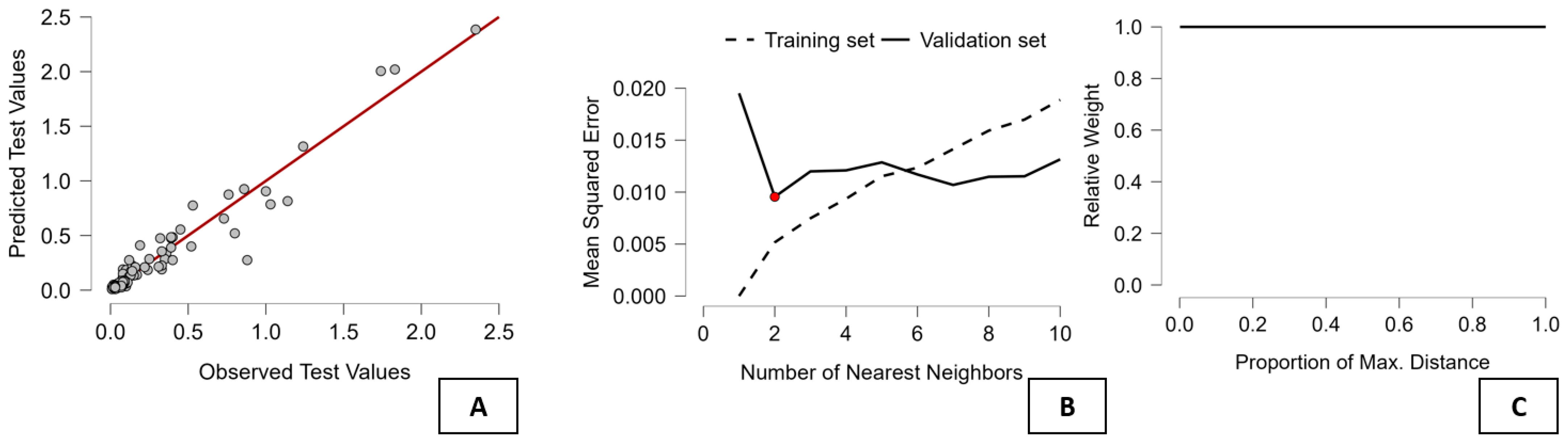
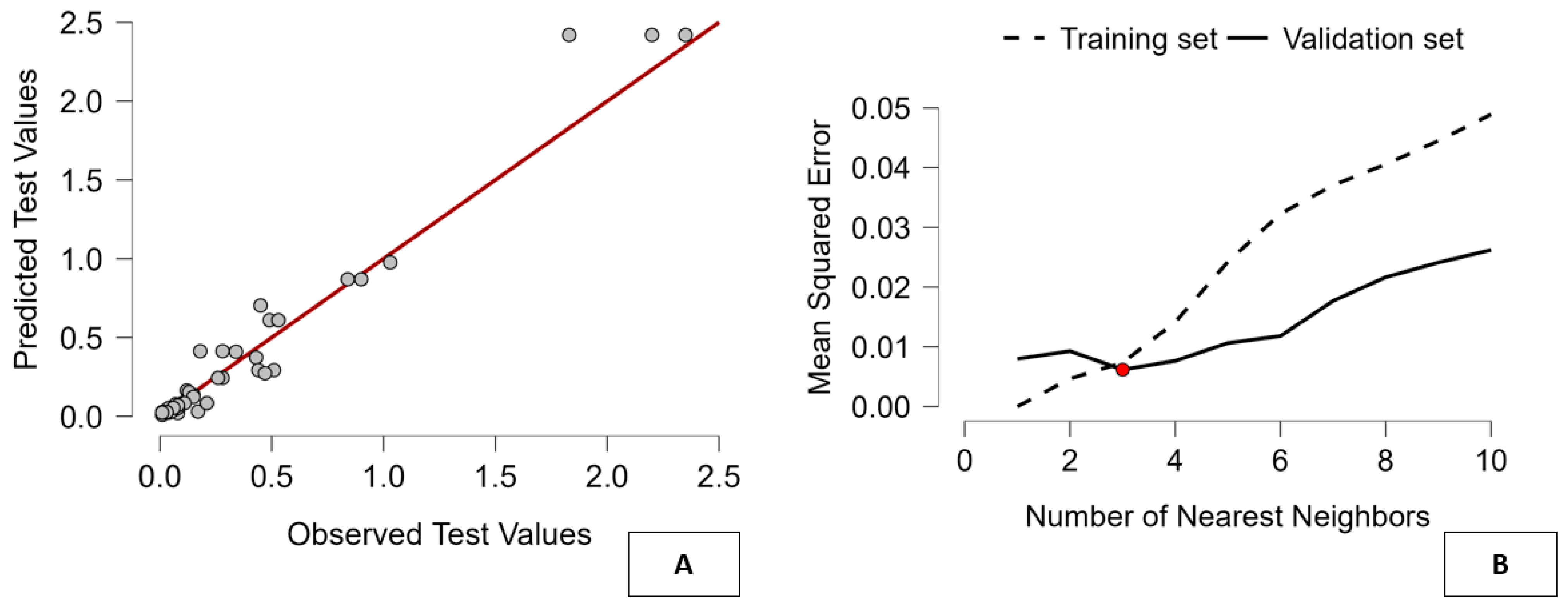
The figure provides a diagnostic summary of the K-Nearest Neighbors algorithm used to estimate geopolitical risk (GPR) based on environmental factors in the ESG model. The three graphs in the figure illustrate the model’s accuracy, the parameter-determination process, and the model’s weighting system. Panel A of the figure illustrates the relationship between the actual GPR values and the model’s predictions for GPR in the test dataset. The scatter diagram in the panel shows a very strong positive linear relationship, with most data points closely aligned along the 45-degree reference line, indicating the model’s ability to accurately reproduce the actual GPR values in the dataset. The deviations from the reference line are small but slightly larger for the data points representing the highest GPR, thus indicating a slight worsening of the model’s prediction accuracy in extreme GPR conditions, which aligns with the expected limitations of the model in extreme conditions based on the established principles of instance-based learning algorithms in model predictions (Kuhn & Johnson, 2019). Panel B focuses on model tuning, plotting the mean squared error against the number of nearest neighbors. The dashed line shows the training error, which increases monotonically with the number of neighbors, as expected with the accompanying increase in bias. The solid line shows the validation error, which decreases to a minimum around 2 nearest neighbors before increasing again. The red dot indicates the optimal value of k that balances bias and variance. This captures the traditional bias-variance trade-off observed in non-parametric machine learning models, indicating that a small neighborhood size is sufficient to identify local data structures (Kuhn & Johnson, 2019). This trend has been observed in applied studies on complex relationships using KNN in machine learning (Garcia Rodriguez et al., 2021). Panel C shows the relative weights of neighbors by distance. The flat line represents uniform weights, which means that each of the selected neighbors has an equal say in the prediction. This selection aligns with the local averaging concept of the KNN algorithm to mitigate the risk of overemphasizing a single observation. From an interpretability perspective, uniform weights make it easier to interpret local predictions. It follows best practices in interpretable machine learning for distance-based algorithms. Together, the above figures show that the KNN model provides calibration, stability, and a strong link between the Environmental aspect of ESG and geopolitical risks. With its high predictability, clear parameters, and weighting, the model is a perfect solution for identifying the nonlinear and specific environmental factors influencing geopolitical risks. See Figure 3.

5. Social Foundations of Geopolitical Risk: An ESG-Based Multi-Method Assessment

In this section, we evaluate the impact of the Social (S) element of the ESG framework on geopolitical risk, as measured by the Geopolitical Risk (GPR) index. The primary research hypothesis is that geopolitical risk stems not only from current political conditions but also from deeper social structures, such as demographically contingent risks, vulnerabilities to labor-market risks, and dynamics of inclusion, which may cumulatively increase a nation’s susceptibility to geopolitical risk. To capture the intricacies of the relationship between these social structures and geopolitical risk, we use a combination of three methods. First, we use a panel data econometric model to estimate a conditional relationship between GPR and a set of social variables such as net migration (MIG), unemployment (UNEM), and population aged 65 years or older (POP65), which are controlled for in a model that also accounts for unobservable country-specific heterogeneity. This allows a meaningful point estimate to be derived, which can be used to evaluate whether a relationship exists between these social factors and the variability of geopolitical risk. Second, we use a clustering analysis to group countries based on additional social factors, such as health, inequality, education, participation, and demographics. These allow for a mean-difference analysis of country-specific groups on GPR to identify which country groups across these additional sets of social factors are associated with varying levels of geopolitical risk. Finally, we use machine learning regression models that focus on non-parametric methods to identify nonlinear relationships between these sets of social factors and geopolitical risk, currently unidentified in standard econometric models.

5.1. Estimating the Social Pillar’s Effect on Geopolitical Risk: A Panel Econometric Approach

To estimate the impact of the S-Social component on geopolitical risk, we estimated the following equation:

$$\mathrm{G}\mathrm{P}{\mathrm{R}}_{\mathrm{i}\mathrm{t}}=\mathsf{\alpha }+{\mathsf{\beta }}_1{\left(\mathrm{M}\mathrm{I}\mathrm{G}\right)}_{\mathrm{i}\mathrm{t}}+{\mathsf{\beta }}_2{\left(\mathrm{U}\mathrm{N}\mathrm{E}\mathrm{M}\right)}_{\mathrm{i}\mathrm{t}}+{\mathsf{\beta }}_3{\left(\mathrm{P}\mathrm{O}\mathrm{P}65\right)}_{\mathrm{i}\mathrm{t}}$$

where $\mathrm{i}$ = 42 and $\mathrm{t}$ = [2000; 2023].

The description of the variables used is given in

Table 11. Social (S) ESG Variables Used in the Geopolitical Risk (GPR) Model.

	Variable	Full Name	Description
Y	GPR	Country GPR—Geo Political Risk	Index measuring a country’s geopolitical risk based on the percentage of news articles related to political tensions, conflicts, and instability.
X	MIG	Net migration	Difference between the number of immigrants and emigrants in a country during a given period, reflecting migration balance and demographic pressure.
	UNEM	Unemployment	Share of the labor force that is without work but actively seeking employment, indicator of economic and social conditions.
	POP65	Population 65+	Percentage of the total population aged 65 years or more, used as a measure of population ageing and demographic structure.

Note: The table defines social variables used to estimate GPR within the ESG framework. Migration, unemployment, and population ageing capture structural social pressures that influence geopolitical risk through demographic dynamics and labor-market conditions.

below.

The study is situated in the Environmental, Social, and Governance (ESG) context, which, in the present day, remains one of the prominent methods for assessing countries’ and their economies’ sustainability and risk profiles (Iwanicz-Drozdowska et al., 2025). The present study focuses primarily on the Social aspect of the Environmental, Social, and Governance criteria and its relationship to demographic and labor-related factors in the context of Geo-Political Risk (GPR). The study uses Geo-Political Risk (GPR) as its dependent variable, which, in turn, serves as an indicator of the number of news articles on conflicts and political instability. The relationship between this GPR and migration rates, unemployment, and an aging population has been used to understand geopolitical risk in terms of social structures (Kharlamova et al., 2025). The panel data consist of 42 countries over 22–24 years, yielding 1006 total data points. Four models have been developed: Fixed Effects, Random Effects GLS, Pooled Ordinary Least Squares, and Weighted Least Squares. The results of the study indicate that the Hausman test overwhelmingly rejects the null hypothesis of GLS estimators, favoring the fixed-effect model, which aligns with the ESG criteria, which state that social factors are mostly explained by differences in institutional structures rather than random variation. The LSDV R-Sq of 0.81 for the fixed-effect model indicates the high explanatory power of structural factors for GPR, and the within R-Sq of 0.02 indicates the importance of short-run social factors. Likewise, joint significance tests for the variables reveal that they are highly significant across all four models, thereby validating the significance of migration, unemployment, and demographic variables for explaining GPR (Onomakpo, 2025). According to the ESG Social perspective, the MIG variable, which stands for net migration, is of particular interest. The migration process is characterized by demographic pressure, labor market opportunities, and social integration capacity (Zatonatskiy et al., 2024). The coefficient for MIG is positive and significant across all models, indicating that net migration is positively correlated with geopolitical risks. This can be explained in different ways: on the one hand, high levels of migration may cause tensions, competition for public resources, and polarization of the electorate in countries with little migration management (Petrović & Vesković Anđelković, 2025). On the other hand, migration may cause conflict, as reflected in geopolitical risks, suggesting a bidirectional relationship between MIG and GPR (Rostetska et al., 2023). The significance of MIG across models highlights the significance of proper migration management within the ESG Social dimension. The coefficient for UNEM, which represents unemployment, is consistently negative and significant across all models, indicating that higher unemployment is associated with lower geopolitical risk. This may seem counterintuitive, but it can be argued that geopolitical risks arise from international tensions rather than internal instability. Countries with lower unemployment may be more engaged in the international economy, which may heighten geopolitical tensions, whereas economic stagnation stemming from high unemployment may lead to lower media coverage, thereby reducing geopolitical risks within the ESG framework. The variable POP65, representing the population aged 65+, has a positive coefficient that is significant in both FE and RE models. Aging populations are usually related to higher levels of geopolitical risk, and this can be attributed to factors such as pressure on welfare, pension, and health systems; intergenerational conflict; lower response to economic changes; and opposition to migration and globalization, which might lead to political instability (Vollset et al., 2020). The importance of POP65 further underscores the role of demographic sustainability in the ESG Social dimension. Diagnostic tests indicate econometric problems with ESG factors. The White and Wald tests indicate rejection of homoskedasticity, suggesting that differences in geopolitical risk are not uniform across countries and are driven by differences in social structures. The Pesaran CD tests are significant, with a p-value close to zero, indicating cross-sectional linkages in factors such as migration crises and labor market shocks, thereby corroborating the ESG Social Pillar’s transnational approach, as discussed in Oliver-Smith (2022). The Wooldridge tests indicate first-order autocorrelation, suggesting a pattern in geopolitical risks over time and indicating that social tensions are cumulative and cannot be easily reversed. Substantively, the findings have several ESG implications. First, it is not possible to consider geopolitical risks in isolation from demographic and labor-market factors, as migration and an aging population are underlying drivers of political instability (Ongan et al., 2025). Second, the S dimension is inextricably linked to political narratives and the media’s perceptions that form the basis of the GPR index. Third, the management of social inclusion and the demographic transition is a primary tool for addressing geopolitical risks. In conclusion, the Social (S) dimension of ESG plays a defining role in managing geopolitical risks. Migration, labor market factors, and an aging population are not simply domestic social factors but also global factors that impact global stability. If countries fail to manage migration, labor markets, and the aging population, political instability may manifest as higher GPR levels. ESG analysis correctly highlights the role of social sustainability in managing geopolitical risks (Kharlamova et al., 2025; Iwanicz-Drozdowska et al., 2025). Improvements in the S dimension of ESG analysis may help reduce geopolitical risks in the globalized world. See

Table 12. Panel Regression Results for the Social (S) ESG Component and Geopolitical Risk (GPR).

Time-Series Length	Minimum 22, Maximum 24
Dependent variable	GPR
Cross-sectional units	42
Observations	1006
Models	Fixed-effects			Random-effects (GLS)			Pooled OLS			WLS
	Coefficient	Std. Error	t-ratio	Coefficient	Std. Error	z	Coefficient	Std. Error	t-ratio	Coefficient	Std. Error	t-ratio
const	0.14 **	0.05	2.57	0.14 *	0.08	1.77	0.26 ***	0.03	7.62	0.11 ***	0.01	8.90
MIG	5.84411 × 10−8 *	3.47289 × 10−8	1.68	8.04722 × 10−8 **	3.43160 × 10−8	2.34	8.12297 × 10−7 ***	3.67460 × 10−8	22.11	2.68920 × 10−7 ***	2.60941 × 10−8	10.31
UNEM	−0.006 **	0.003	−2.21	−0.006 **	0.002	−2.24	−0.01 ***	0.002	−4.03	−0.003 ***	0.0008	−4.37
POP65	0.01 ***	0.003	2.87	0.01 ***	0.003	2.93	−0.001	0.002	−0.57	0.001	0.0007	1.40

Note: The table reports panel estimates linking social factors to geopolitical risk. Migration, unemployment, and population ageing capture social security pressures affecting stability, indicating that improvements in the ESG Social component can mitigate geopolitical risk in a globalized context. *** p < 0.01, ** p < 0.05, * p < 0.10.

.

Addressing Cross-Sectional Dependence, Endogeneity, and Serial Correlation in Panel Models. However, given the global nature of the dataset, with 42 countries observed over 24 years, several econometric problems arise, including cross-sectional dependence, heteroskedasticity, serial correlation, and endogeneity. The concerns are particularly pertinent to geopolitical risks, given their worldwide nature, including global financial crises and migration flows. The presence of cross-sectional dependence is confirmed through diagnostic tests. The CD test statistics robustly reject the null hypothesis of cross-sectional independence (Pesaran CD test statistics z = 38.4238, p-value = 0). The rejection of the null hypothesis suggests that country-specific shocks are not independent but rather correlated, in line with the observed high level of economic and political integration across all countries in our sample. In addition, heteroskedasticity in our panel data is confirmed by distribution-free Wald tests (χ²(42), 668,171, p-value = 0), suggesting that the error term variance varies across cross-sectional units. Serial correlation in panel data is confirmed by the Wooldridge test for autocorrelation (F(1, 41) = 7.32631, p-value = 0.0099), suggesting that the error structure is persistent over time. To address all econometric concerns in our panel data, our primary regression employs a fixed effects (FE) estimator with HAC-robust standard errors to correct for heteroskedasticity and serial correlation. The test for differing group intercepts in our panel data rejects the hypothesis at the 0.01 significance level (Welch F = 44.1097, p-value < 0.001), warranting the use of fixed effects, as it indicates heterogeneity in panel data intercepts. In addition, the Hausman specification test (χ²(3) = 21.6305, p-value < 0.001) rejects the hypothesis that unobservable factors are uncorrelated with regressors in panel data, thus supporting the consistency of fixed effects relative to random effects in panel data analysis. However, though it improves inference quality by using first-generation panel-data estimators and robust standard errors, cross-sectional dependence due to common unobservable factors remains a concern. Therefore, a possible extension of this study could be to expand the model using second-generation panel data methods, such as Common Correlated Effects (CCE) and Driscoll–Kraay standard errors, to correct for cross-section correlations arising from global shocks. The endogeneity of variables, such as the unemployment variable UNEM and the population aging variable POP65, could be affected by geopolitical instabilities. Instrumental variable methods are used for addressing endogeneity and reverse causality concerns using the Fixed Effects 2SLS and Random Effects G2SLS models. Climatic and environmental variables such as SPEI, WSTR, WAT, LST, CDD, and HDD are used as instrumental variables, as they affect social pressures but not geopolitical risks, except through these channels. The TSLS results confirm a positive and significant impact of population aging on geopolitical risks, whereas the impact of the unemployment variable depends heavily on the model specification. However, it is noteworthy that the Wald statistic values are very low. Geopolitical risks, as measured by GPR, still persist, and, given the concern about serial correlation, further improvements could be achieved by using system GMM methods such as the Arellano-Bover/Blundell-Bond estimators, which correct for endogeneity and reverse causality arising from lagged dependent variables. The above study presents a comprehensive model while acknowledging other possible avenues for further exploration in the context of second-generation and dynamic panel data methods. See

Table 13. Panel Regression Results with Fixed Effects and Instrumental Variable Estimators.

Section	Item	Model 1—FE (HAC)	Model 2—FE-TSLS	Model 3—RE-G2SLS
General Info	Observations	1006	861	861
	Cross-sectional units	42	42	42
	Time-series length	22–24	13–21	13–21
	Dependent variable	GPR	y	y
	Estimator	Fixed Effects (LSDV)	Fixed Effects TSLS	Random Effects G2SLS
	Robust SE	HAC	Yes	Yes
	Endogenous variables	—	UNEM, POP65	UNEM, POP65
	Instruments	—	SPEI, WSTR, WAT, LST, CDD, HDD	SPEI, WSTR, WAT, LST, CDD, HDD
Coefficients	const	0.143954 (0.0820808) p = 0.0869	−0.808788 (0.501052) p = 0.1065	−0.358175 (0.277254) p = 0.1964
	UNEM	−0.00674719 (0.00466180) p = 0.1554	0.0583873 (0.0320673) p = 0.0686	0.0257912 (0.0237899) p = 0.2783
	MIG	5.84411 × 10−8 (3.99955 × 10−8) p = 0.1516	—	—
	POP65	0.0108993 (0.00584574) p = 0.0694	0.0487141 (0.0228797) p = 0.0332	0.0318929 (0.0149782) p = 0.0332
Model Fit & Stats	Mean dep. var	0.232197	—	—
	S.D. dep. var	0.457230	—	—
	SSR	38.17959	40.0517	618.942
	S.E. regression	0.199321	—	—
	sigma-hat	—	0.221411 (df = 817)	0.84934 (df = 858)
	sigma-hat (within)	0.13507279	0.22141125	—
	sigma-hat (between)	0.44975072	0.4109164	—
	R-squared	LSDV 0.818283; Within 0.021484	0.001120	0.000998
	Log-likelihood	218.0802	—	—
	Akaike	−346.1605	—	—
	Schwarz	−125.0423	—	—
	Hannan-Quinn	−262.1446	—	—
	rho	0.426115	—	—
	Durbin-Watson	1.079741	—	—
	Wald χ2	—	4.53341 (p = 0.1037)	5.05168 (p = 0.0800)
Diagnostic Tests	Joint test regressors	F(3, 41) = 2.19173 (p = 0.10358)	—	—
	Group intercepts test	Welch F(41,336.2) = 44.1097 (p = 2.7398 × 10−111)	F(41,817) = 67.8359 (p = 0.0000)	—
	Heteroskedasticity	χ2(42) = 668,171 (p = 0)	—	—
	Normality	χ2(2) = 1405.14 (p = 7.53969 × 10−306)	—	—
	Wooldridge autocorrelation	F(1, 41) = 7.32631 (p = 0.00986009)	—	—
	Pesaran CD	z = 38.4238 (p = 0)	—	—

Note. The table reports panel regression estimates using fixed-effects models with HAC-robust standard errors and instrumental variable techniques (FE-TSLS and RE-G2SLS) to address heteroskedasticity, serial correlation, and potential endogeneity in unemployment and population ageing variables.

.

5.2. Clustering Social Structures and Geopolitical Risk: A Comparative Algorithmic Assessment

However, the choice of the best clustering algorithm should be based on a fair consideration of all normalized measures, with a focus on both the quality and the balance of the resulting clusters. Since each metric is normalized so that the best result is higher, it is easy to compare results across algorithms. The hierarchical algorithm shows a marked superiority in the internal quality of the resulting clusters, achieving the highest values for minimum separation, Pearson’s γ, Dunn’s index, and entropy, which are combined indicators of highly compact, well-separated, and internally consistent clusters (Hindupur et al., 2025). This level of superiority comes with a significant disadvantage: the HH index for the hierarchical algorithm is zero, indicating that the data points are highly concentrated around a few clusters. This level of imbalance makes the result less interpretable and less useful, especially for situations that call for a relatively balanced partitioning of the data points. On the contrary, the density-based algorithm shows the greatest balance in cluster sizes, achieving the highest HH index value (Hindupur et al., 2025). This level of balance comes with remarkably low structural superiority across all metrics, which are combined indicators of the level of separation and internal cohesion of the resulting clusters (Hindupur et al., 2025). This indicates that while the algorithm produces a relatively balanced number of data points, the resulting data points are evenly distributed without any clear level of separation and internal cohesion. k-Means performs well on the Calinski-Harabasz index, as well as on Pearson’s γ, but has a rather low HH index, indicating a preference for the concentration of observations into larger clusters. Model-based and Fuzzy C-Means methods yield medium values, neither of which is outstanding in either structural quality or balance. Random Forest-based clustering is clearly the most balanced approach. Although it is not outstanding on any of the individual criteria, it is always close to the best values on all of them. In particular, it combines good separation and compactness (Dunn index, Pearson’s γ, Minimum separation) with an extremely high HH index, an important indicator of a balanced distribution of observations across clusters (Sondag et al., 2025). This is particularly important if the aim is to identify a heterogeneous structure without allowing a single cluster, or a small set of clusters, to dominate the others. Considering both clustering quality and concentration, Random Forest is clearly the best-performing algorithm, providing the best balance among the considered approaches (Sondag et al., 2025; Hindupur et al., 2025). See

Table 14. Comparative Clustering Performance Across Algorithms for the Social (S) ESG Dimension.

Metric	Density Based	Fuzzy C-Means	Hierarchical	Model Based	k-Means	Random Forest
Maximum diameter	0.01	0.58	1.00	0.00	0.80	0.74
Minimum separation	0.07	0.00	1.00	0.56	0.20	0.56
Pearson’s γ	0.00	0.32	1.00	0.08	0.62	0.29
Dunn index	0.02	0.00	1.00	0.35	0.15	0.46
Entropy	0.00	0.56	1.00	0.74	0.55	0.45
Calinski–Harabasz index	0.00	0.31	0.26	0.09	1.00	0.49
HH index	1.00	0.75	0.00	0.56	0.71	0.86

Note: Random Forest clustering offers the best overall balance between cluster quality and concentration, combining strong separation and compactness with a high HH index, ensuring heterogeneous yet well-balanced clusters without dominance by few groups.

.

The results of the Random Forest clustering method indicate that the association between the Social (S) factor of Environmental, Social, and Governance (ESG) ratings and geopolitical risks (GPR) is complex. The model includes various social, demographic, health, and other indicators to segment the countries into groups, highlighting the social characteristics of each group. Standardized scores have been utilized to highlight differences between clusters. Countries in clusters 1 and 6, where geopolitical risks are lower or negative, have stronger social foundations in Economic and Social Rights (ESR), higher access to public services in education and healthcare facilities, lower levels of undernourishment (UND), lower child mortality rates (U5MR), and higher female labor force participation (FLFP). However, life expectancy at birth (LEX) could be lower owing to demographic factors, yet clusters 1 and 6 reveal more cohesive and inclusive social structures. The implications for ESG ratings highlight that more inclusive, less unequal, and more robust social welfare systems could reduce geopolitical risks (Larson et al., 2025; Koumpagioti et al., 2025). In conclusion, the Random Forest clustering analysis supports the view that geopolitical risk is inextricably linked to social structures. Inequality, exclusion, poor health and education infrastructure, and population-related stressors increase vulnerability, while strong and inclusive social structures and development reduce vulnerability (Rao et al., 2023; Gebreegziabher et al., 2024). The most significant result is the importance of the Social (S) element of ESG criteria for rating GPR, with the need for policies that support social equity, health, education, and development for long-term geopolitical stability (Larson et al., 2025; Koumpagioti et al., 2025). See

Table 15. Social (S) ESG Clusters and Geopolitical Risk (GPR): Cluster-Level Standardized Indicators.

	GPR	ESR	FER	FPI	GINI	GEDU	HOSP	INC20	INT	LFP	LEX
Cluster 1	−0.984	0.763	−0.681	−0.310	1.173	1.700	0.410	−0.493	−0.782	−1.563	−0.742
Cluster 2	0.735	−0.196	0.587	−0.089	0.029	−0.213	−0.053	0.795	−0.556	0.151	0.831
Cluster 3	0.539	0.116	0.360	0.159	−0.713	−0.679	1.356	0.276	0.849	0.686	0.519
Cluster 4	−0.395	0.028	−0.652	−0.025	−0.319	0.755	−0.600	1.514	0.056	−0.753	−0.440
Cluster 5	0.909	−0.084	0.889	0.016	−0.237	−1.067	0.379	−0.476	−0.198	1.128	1.037
Cluster 6	−1.935	1.122	−1.299	0.292	1.003	0.183	−0.134	−0.422	−1.164	0.315	−1.806
Cluster 7	0.168	−0.788	0.197	0.260	−0.437	−0.456	−0.921	−0.008	1.536	0.459	0.789
Cluster 8	−0.054	−0.946	0.164	−0.605	−0.164	−0.808	−0.453	−0.403	1.278	0.767	−0.494
Cluster 9	0.341	2.780	0.529	−0.157	1.428	0.801	0.285	0.388	−0.390	−1.259	0.147
Cluster 10	0.453	−1.053	−0.106	0.492	−0.961	0.028	−0.252	−0.384	−0.374	−0.410	−0.208
	U5MR	MIG	POP65	PDEN	OVW	UND	WIP	FLFP	PRIM	GPI	UNEM
Cluster 1	−0.811	−0.312	−0.457	0.719	−0.821	−1.271	0.764	0.915	0.533	−0.122	−0.144
Cluster 2	0.649	0.674	0.538	0.769	−0.098	0.293	−0.356	−0.404	−0.359	−0.128	−0.165
Cluster 3	0.692	−0.465	−0.125	−0.572	0.808	0.627	−0.128	−0.504	−0.359	0.310	0.468
Cluster 4	−0.698	−0.559	1.003	0.210	−0.503	−0.724	−0.340	0.306	−0.340	−0.095	−0.816
Cluster 5	0.619	0.925	−0.209	−0.083	−0.114	0.570	0.012	−0.602	−0.359	−0.312	1.269
Cluster 6	−1.628	−0.724	−0.553	−1.653	0.334	−1.534	0.766	2.112	2.665	−0.745	−1.032
Cluster 7	0.835	0.978	0.369	−0.745	0.837	1.194	−0.031	−0.542	−0.348	−0.642	0.079
Cluster 8	−0.886	−0.771	−0.299	0.425	−0.269	0.225	−0.727	−0.176	−0.359	0.185	−1.077
Cluster 9	0.794	0.020	−0.284	0.358	1.816	−0.775	−1.164	−0.504	−0.359	−0.173	−0.420
Cluster 10	0.762	−0.291	0.027	0.135	−0.031	0.957	0.197	−0.569	−0.359	1.537	0.464

Note: Clusters with higher labor force participation and female-to-male participation show lower GPR. Social inclusion, equality, health, and education reduce vulnerability, while inequality, exclusion, and demographic stress raise geopolitical risk, confirming GPR’s deep social foundations globally.

.

The results of the Random Forest clustering analysis provide insight into the specific role of the Social (S) component in the ESG model relative to geopolitical risk (GPR). The model’s results, as measured by average Gini reduction values, provide insight into which social factors are most important in determining groupings based on geopolitical risk. Rather than a linear relationship between social factors and geopolitical risk, the results suggest that the social factors are most important in determining a country’s geopolitical risk profile. The most important factors relate to health outcomes, population characteristics, and inequality. Notably, the under-5 mortality rate (U5MR) is identified as the most important factor in assessing geopolitical risk. This is consistent with the idea that healthcare is a critical component in determining geopolitical risk. High rates of child mortality are a reflection of poor healthcare systems and a lack of access to essential services, which can contribute to geopolitical instability and risk (Rangachari & Thapa, 2025; Crawshaw & Gray, 2025). The prominence of population ageing (POP65) further supports the connection between demographic imbalance and geopolitical risk (Lakioti et al., 2025). Additionally, a strong link exists between inequality and geopolitical risk, indicated by the Gini index (GINI) and income distribution to the bottom 20 percent (INC20). Increased inequality can foster social instability and compromise political systems, thereby increasing geopolitical risks (Lompo & Diendere, 2025). On the other hand, the emphasis on economic and social rights (ESR) performance and their relationship to increased life expectancy (LEX) suggests a stabilizing effect of social development on geopolitical risk. The emphasis on human capital participation variables confirms these findings. Variables such as internet use (INT), female and total labor force participation (FLFP, LFP), education expenditure (GEDU), school enrollment (PRIM and GPI), and female representation in Parliament (WIP) reflect high social inclusion and access to knowledge, supporting social stability and lower geopolitical risk (Lakioti et al., 2025). Labor market dynamics and demographic factors also shape differences across clusters. The variables unemployment (UNEM), fertility rate (FER), migration (MIG), and population density (PDEN) suggest a high level of resource competition and geopolitical instability in a society characterized by high unemployment and demographic change. Uncontrolled migration can exacerbate geopolitical instability and social and political tensions in a society and globally (Vesco et al., 2025). In conclusion, the Random Forest clustering results affirm the pivotal role of geopolitics in the overall social structure. Health, inequality, demographics, education, and social activities are not peripheral but rather key components of GPR. Within the ESG model, the Social component serves as a foundational base for managing geopolitical risks and complements the Environmental and Governance factors. Policies aimed at improving social progress, equality, health, education, and inclusion are justified on social grounds and necessary to reduce geopolitical risks (Lakioti et al., 2025; Lompo & Diendere, 2025). See

Table 16. Ranking of Social ESG Indicators Influencing Geopolitical Risk (GPR).

Feature Importance	Mean Decrease in Gini Index	Feature Importance	Mean Decrease in Gini Index
U5MR	23.097	GEDU	13.975
POP65	22.210	LFP	13.515
GINI	21.066	PDEN	12.408
ESR	20.532	OVW	12.281
INT	18.356	MIG	11.162
LEX	18.348	PRIM	9.745
INC20	17.162	UNEM	9.303
FLFP	16.647	GPI	8.590
HOSP	16.244	UND	8.250
FER	14.986	GPR	8.102
WIP	14.054	FPI	6.520

.

Figure 4 illustrates the application of Random Forest clustering to the Social (S) aspect of ESG analysis, specifically to investigate its relationship with geopolitical risk (GPR). Together, the two panels in this figure illustrate both the model selection step and the resulting clustering. Panel A illustrates the criteria used to determine the appropriate number of clusters to retain in this analysis. In this panel, note that both the Within Sum of Squares (WSS) and the AIC and BIC measures decrease continuously with an increase in the number of clusters, indicating a corresponding improvement in homogeneity within each cluster. Also, in this panel, a red spot marks the minimum BIC point obtained with 10 clusters. This finding suggests that a ten-cluster solution is preferred for a balance between simplicity and explanatory power, allowing meaningful differentiation in social conditions without overfitting to observations on geopolitical risk (Taye et al., 2025). Panel B in this figure shows a two-dimensional representation of the clustering result obtained using a Random Forest method. Each point in this panel represents an observation characterized by a very large number of social variables, including health metrics, levels of inequality, educational levels, demographic characteristics, and measures of social inclusion. In this panel, different clusters are colored to distinguish them based on their differences in social variables, using a ten-cluster solution derived from a Random Forest method developed in this analysis. These clusters appear compact and well-separated in this panel, indicating that this method has been highly effective at distinguishing different social characteristics (Sahin, 2025). These characteristics differ in terms of varying degrees of vulnerability and resilience that influence differences in geopolitical risk (Taye et al., 2025). From this figure, it is clear that a Random Forest method is highly effective at capturing nonlinear relationships among social variables that contribute to geopolitical risk (Taye et al., 2025). This analysis has distinguished different regimes within a broader ESG analysis, reaffirming the finding that geopolitical risk is deeply embedded in social structures such as those based on inequality, health, education, and demographics (Bendavid et al., 2025; Sahin, 2025). See Figure 4.

Social Dimension and Domestic Stability Mechanisms. The cluster analysis of social dynamics shows that geopolitical risk is embedded in the country’s social structures. Specifically, clusters with high Global Political Risk (GPR) levels are associated with high inequality, demographic pressures, unemployment, undernourishment, and lower health and education standards, whereas clusters with high social rights, high female labor force participation, and better health and education standards consistently exhibit lower GPR levels. Differentiators for critical regimes include child mortality, income distribution, and migration flows. This contrast confirms that lower social cohesion reduces internal resilience and amplifies external geopolitical pressures, while social stability operates mainly through internal mechanisms. Thus, high social resilience reduces GPR levels. In other words, geopolitical risk is tied not only to external factors but also to internal social structures.

5.3. Predicting Geopolitical Risk from Social ESG Factors: A Machine Learning Comparison

As illustrated in the table of normalized performance above, the KNN algorithm performs better than the other algorithms. It should be noted, however, that the normalization was performed so that higher values indicate better performance. Moreover, error-based performance metrics, including MSE, scaled MSE, RMSE, MAE/MAD, and MAPE, have been set to be minimized, and R² has been set to be maximized. According to the results, under a uniform performance evaluation criterion, the best-performing model attains a score of 1.00 across all metrics, indicating optimal performance in terms of error and goodness-of-fit. This aligns with prior studies, which have identified the KNN model as one of the best-performing in various fields, including energy forecasting and epidemiology (Rakshit & Sengupta, 2024; Kaliappan et al., 2021). Thus, the KNN model has been identified as the best-performing model in the competition, without compromising accuracy and interpretability, while the performance of the other models has been found less consistent. Among the alternative models, the Support Vector Machines (SVMs) offer the highest performance in terms of error metrics, where the highest score is 0.92 for MSE, 0.78 for RMSE, 0.76 for MAE/MAD, and 0.63 for MAPE, in addition to the highest performance in terms of explanatory performance, as indicated by the R² score of 0.59. The regularized linear models offer acceptable performance in terms of error metrics, where the highest score is 0.85 for MSE, but poor performance in terms of explanatory performance, where the R² score is 0.28. The Random Forest model shows acceptable explanatory performance (R² = 0.78), but poor performance in other metrics, with the lowest MAPE score of 0.39 compared to the SVM and KNN models. The Linear Regression model shows average performance across all metrics, whereas the Boosting model shows poor performance in scaled MSE and a low R² score under the normalized evaluation criteria (Sibai et al., 2024). The Decision Tree model indicates poor performance, with a score of 0.00 across all metrics. The results suggest that the KNN model should be chosen for the task, given the need to optimize performance across different error metrics and to achieve the highest explanatory performance. The high performance of the KNN model across all metrics is in line with its robustness and suitability for continuous prediction, as well as its error metrics (Rakshit & Sengupta, 2024; Sibai et al., 2024). See

Table 17. Comparative Predictive Performance of Machine-Learning Models for the Social (S) ESG–GPR Framework.

Metric	Boosting	Decision Tree	KNN	Linear Regression	Random Forest	Regularized Linear	SVM
MSE	0.71	0.00	1.00	0.75	0.71	0.85	0.92
MSE (scaled)	0.00	—	1.00	0.76	0.81	0.40	0.69
RMSE	0.52	0.00	1.00	0.56	0.52	0.68	0.78
MAE/MAD	0.46	0.00	1.00	0.43	0.58	0.62	0.76
MAPE	0.54	0.00	1.00	0.43	0.39	0.57	0.63
R2	0.00	—	1.00	0.70	0.78	0.28	0.59

Note: KNN delivers the strongest overall performance, combining the lowest errors with the highest explanatory power. Random Forest shows good fit but weaker error metrics, Linear Regression performs moderately, while Boosting and Decision Tree models display limited explanatory capacity.

.

The above findings highlight the importance of features, as determined by the mean dropout loss, which represents the level of degradation in prediction performance when each feature is removed. As such, the features with higher values indicate the most impactful social factors in explaining Geopolitical Risk (GPR) within the Social (S) dimension of ESG. The results show that net migration (MIG) is the most significant feature by a wide margin, implying that migration trends are among the primary factors influencing Geopolitical Risks. Migration can be an indicator of economic, political, and social pressure in countries, as well as an accelerator of Geopolitical Risks by instigating distributional conflicts, political polarization, and interstate conflicts (Zatonatskiy et al., 2024). Variables such as population density (PDEN), fertility rate (FER), and the proportion of the population that is overweight (OVW) exhibit strong correlations among themselves, suggesting they form a demographic pressure indicator. As such, countries with rapid population growth, high population density, or changes in health/nutrition status tend to have higher levels of geopolitical risk. These factors can be viewed as stressors on the population, exacerbating instability in the country (Conduah & Ofoe, 2025). The importance of labor market indicators and economic inclusion factors should also be recognized as significant. The importance of Unemployment (UNEM), Income Share of the Lowest 20 Percent (INC20), Gini Index (GINI), and Economic and Social Rights (ESR) is considerable, thereby reiterating the centrality of inequality and exclusion as key social determinants of geopolitical risk. Societies characterized by high inequality and limited economic opportunities tend to be more prone to social unrest, institutional trust decay, and political fragmentation (Zatonatskiy et al., 2024). Human capital, characterized by access to services, education, and healthcare, has been recognized as pivotal in shaping geopolitical risk. Government expenditure on education (GEDU), primary school enrollment rate (PRIM), gender parity in education (GPI), number of hospital beds per 1000 population (HOSP), life expectancy at birth (LEX), and under-five mortality rate (U5MR) have been recognized to indicate considerable differences in healthcare and education infrastructure, which have been regarded to considerably affect geopolitical risk. Lastly, inclusion and participation indicators, including internet access (INT), women’s parliament representation (WIP), women’s workforce participation (FLFP), and workforce participation (LFP), have been recognized to highlight the importance of social inclusion. The results have robustly established that the roots of geopolitical risk lie in social structures. Migration, inequality, population, health, education, and workforce participation have been regarded as the key determinants of the Social component of ESG, which defines GPR (Zatonatskiy et al., 2024; Blukacz et al., 2025; Conduah & Ofoe, 2025). See

Table 18. Social (S) ESG Feature Importance for Geopolitical Risk (GPR) Based on Mean Dropout Loss.

Feature Importance Metrics	Mean Dropout Loss	UND	0.089
MIG	0.355	INC20	0.088
PDEN	0.116	INT	0.088
FER	0.111	WIP	0.088
OVW	0.110	U5MR	0.087
UNEM	0.102	POP65	0.086
FPI	0.095	GINI	0.086
GEDU	0.094	ESR	0.086
HOSP	0.093	LFP	0.085
LEX	0.090	FLFP	0.085
GPI	0.089	PRIM	0.085

Note. Social inclusion mitigates geopolitical risk through stronger cohesion. Migration, inequality, population pressure, health, education, and participation emerge as key Social ESG drivers shaping GPR, confirming geopolitical risk as structurally embedded within social systems.

.

The above results can be viewed as providing a localized understanding of the K-Nearest Neighbors (KNN) algorithm’s predictions regarding the role of the Social (S) dimension in the ESG model and its impact on Geopolitical Risk (GPR). As shown in the five cases, the predicted GPR is expressed as a deviation from a standard baseline of 0.210, and the impact of the individual social variables on GPR is similarly expressed. An interesting aspect of the five cases is that the GPR is consistently lower across them, albeit to varying degrees. This implies that the overall impact of the social variables in each case is to reduce the GPR rather than to elevate it. Variables related to education, the economy, and human capital play a prominent role in the ESG model. Variables such as government expenditure in education (GEDU), labor force participation (LFP), primary school enrollment, gender parity in education (PRIM, GPI), and internet usage (INT) make negative contributions to the KNN algorithm’s predictions. This implies that the higher the level of educational development and internet usage, the lower the GPR (Shergill et al., 2025). From an ESG perspective, the above results lend support to the notion that societies with higher levels of human capital are better able to cope with the risks posed by geopolitical events (Seow, 2025). Finally, the state of labor markets and social inclusion is also a critical factor. UNEM, INC20, and FLFP always have a significant impact on reducing GPR expectations, especially when the initial risk is lowest. This further confirms the notion of a more cohesive, unified political system arising from an inclusive and equitable society and labor market. This is also supported by Dincă et al. (2025). Finally, demographic and migration trends also appear to be critical components of this model. MIG has a strong negative impact on GPR expectations across all scenarios, suggesting a positive relationship between effective migration and geopolitical risk. Fertility rates (FERs), population aging (POP65), and population density (PDEN) have a smaller impact on GPR expectations but still confirm a positive relationship between demographic imbalance and GPR. This may not be as direct a relationship as some of the other components on GPR minimization. Finally, measures of health and social well-being, such as life expectancy (LEX), under-five mortality rate (U5MR), and hospital infrastructure (HOSP), are also critical components of minimizing geopolitical risk. This is because they measure a society’s ability to deliver fundamental welfare and care services and to protect its citizens, which can directly affect geopolitical risk. In total, these results confirm that GPR remains closely linked to social factors and that improvements in education, healthcare, and social and demographic well-being can reduce GPR expectations. This is critical to ESG risk assessment because it confirms the Social dimension’s critical role in minimizing geopolitical risk, alongside environmental and governance factors. See

Table 19. Local Social Contributions to Predicted Geopolitical Risk (GPR) Across Five Cases.

Case	Predicted	Base	ESR	FER	FPI	GINI	GEDU	HOSP	INC20	INT	LFP
1	0.020	0.210	−0.008	−0.001	−0.004	−0.002	−0.010	−6.076 × 10−4	−0.014	−8.210 × 10−5	−0.009
2	0.020	0.210	0.007	0.010	−0.013	8.210 × 10−4	−0.010	−1.642 × 10−5	0.020	4.598 × 10−4	−0.017
3	0.077	0.210	−0.004	−0.012	−0.035	0.000	0.002	−0.011	0.005	−0.001	−0.018
4	0.163	0.210	−9.852 × 10−4	−0.004	−0.035	0.052	−0.002	−0.007	−0.008	0.006	−0.018
5	0.040	0.210	−0.015	−4.105 × 10−4	0.005	2.299 × 10−4	−0.027	0.002	0.003	−0.116	−0.026
LEX	U5MR	MIG	POP65	PDEN	OVW	UND	WIP	FLFP	PRIM	GPI	UNEM
−0.006	0.000	−0.041	0.005	−0.020	−0.017	4.433 × 10−4	−0.009	−0.002	−0.037	−0.013	−3.777 × 10−4
0.015	3.284 × 10−5	−0.041	0.010	−0.020	−0.034	8.210 × 10−5	−0.029	−0.001	−0.018	−0.033	−0.035
−0.002	0.001	−0.041	−0.009	0.037	−0.014	1.314 × 10−4	−0.007	−0.004	5.583 × 10−4	−0.015	−0.005
0.001	0.002	−0.041	9.852 × 10−4	0.029	−0.016	8.867 × 10−4	1.806 × 10−4	8.210 × 10−5	9.524 × 10−4	−0.006	2.463 × 10−4
0.019	1.149 × 10−4	−0.045	0.029	−0.022	−0.046	9.195 × 10−4	0.141	−0.011	−0.055	−0.010	0.003

Note. KNN results show GPR is strongly shaped by social conditions. Improvements in education, healthcare, inclusion, and demographic balance consistently reduce GPR, confirming the Social ESG pillar as a core determinant of long-term geopolitical stability.

.

Figure 5 evaluates the performance and parameter tuning of the K-Nearest Neighbors (KNN) algorithm, focusing on the Social (S) dimension within the ESG analysis framework and its role in shaping geopolitical risk (GPR). The two graphs provide complementary insights into the model’s predictive accuracy. Graph A illustrates the relationship between the actual and predicted GPR in the test data. The scatter chart shows an excellent fit of the data points to the 45-degree reference line. This implies that the KNN model has successfully predicted actual levels of GPR in the data (Baihaqi & Fakhriza, 2025). Most data points lie very close to the reference line, especially in the lower-to-medium GPR range. This implies that the model has captured the role of the S dimension in shaping GPR in standard situations. Small departures from the reference line in the high-GPR range indicate uncertainty in the model’s predictions of extreme GPR (Trianda et al., 2025). Panel B focuses on the process of choosing the optimal number of nearest neighbors. The dotted line in the graph marks the training error, whereas the solid line marks the validation error. As expected, the training error tends to increase with the number of neighbors, indicating greater bias, whereas the validation error first decreases and then increases. The minimum point of the validation error, marked by the red spot, typically occurs when the number of neighbors is small. The results indicate that a local model performs best, consistent with the idea that geopolitical risk is a function of country-specific social factors, such as inequality, healthcare, education, and demographics (Saltık, 2024). In general, the figure above supports the use of KNN for modeling the nonlinear, localized impacts of social variables on geopolitical risk within the ESG framework. The use of the ESG framework, which is characterized by its complexity, requires the use of models that have the properties of being able to predict well, being transparent, and being able to respond well to localized conditions, as in the case of the KNN model, which is sensitive to the mentioned properties (Trianda et al., 2025; Baihaqi & Fakhriza, 2025). See Figure 5.

6. Governance as a Structural Driver of Geopolitical Risk: An ESG Perspective

This section analyzes the role of Governance (G) in ESG in the context of Geopolitical Risk (GPR) and further elucidates its relationship with GPR by emphasizing the influence of institutional quality on a country’s susceptibility to GPR. The basic assumption is that a country’s susceptibility to GPR is influenced by both international and political factors, as well as its foundational structures, which shape its overall resilience and position in international politics. The model integrates a holistic approach that combines three methodologies to further elucidate the relationship between GPR and Governance, and how it is influenced by factors such as control of corruption, political stability, and innovation, among others, while controlling for country-specific and time-specific factors. The panel econometric model is used to estimate the average relationship between GPR and key factors in Governance, such as control of corruption, political stability, and innovation, among others, and further assess its relationship with GPR, in order to establish a clear benchmark that can be used to assess if there is a relationship between Governance quality and GPR. The clustering methodology is further used to cluster countries based on a broad range of factors, such as institutional quality and innovation, among others, in order to establish different regimes in Governance and further assess how GPR levels are related to each regime, in a bid to further elucidate the G-Governance → GPR relationship in a structured ESG model that integrates inference, recognition, and prediction.

6.1. Modeling the G–GPR Link: Corruption Control, Political Stability, and Innovation Capacity in Panel Regression

Below we analyse the impact of the G-Governance component within the ESG context on the GPR variable or geopolitical risk through the estimation of the indicated equation:

$$\mathrm{G}\mathrm{P}{\mathrm{R}}_{\mathrm{i}\mathrm{t}}=\mathsf{\alpha }+{\mathsf{\beta }}_1{\left(\mathrm{C}\mathrm{O}\mathrm{R}\right)}_{\mathrm{i}\mathrm{t}}+{\mathsf{\beta }}_2{\left(\mathrm{P}\mathrm{S}\mathrm{A}\mathrm{V}\right)}_{\mathrm{i}\mathrm{t}}+{\mathsf{\beta }}_3{\left(\mathrm{S}\mathrm{T}\mathrm{J}\mathrm{A}\right)}_{\mathrm{i}\mathrm{t}}$$

where i = 42 and t = [2000; 2023]. The variables used in the model are summarized in

Table 20. Governance (G) ESG Variables Used in the Geopolitical Risk (GPR) Model.

Variable	Full Name	Description
GPR	Country GPR—Geo Political Risk	Index measuring a country’s geopolitical risk based on the percentage of news articles related to political tensions, conflicts, and instability.
COR	Control of Corruption	Indicator measuring the extent to which public power is exercised for private gain, including both petty and grand forms of corruption, and the effectiveness of anti-corruption policies.
PSAV	Political Stability	Measure of the likelihood of political instability, government disruption, or violence, including terrorism and social unrest.
STJA	Scientific & Technical Articles	Number of scientific and technical journal articles published, used as a proxy for innovation capacity and knowledge development in a country.

Note. The table defines governance indicators used to assess GPR within the ESG framework. Control of corruption, political stability, and innovation capacity capture institutional quality, highlighting how effective governance structures contribute to lower geopolitical risk and greater resilience.

below.

The current study explores the relationship between geopolitical risk and a range of variables in the Governance dimension of ESG. Geopolitical risk (GPR) is used as a dependent variable, measured as an index of risk in a particular country based on the number of news articles related to political tensions, conflicts, and instability (Ferreira et al., 2023). Explanatory variables include a range of characteristics related to governance in terms of Control of Corruption, Political Stability, and the number of Scientific and Technical Articles, which can be seen as an indicator of capabilities for innovation and development in institutions (Babarinde et al., 2025). The purpose of the current study is to shed light on the relationship between existing governance structures and geopolitical risk resilience (Reyad et al., 2024). The dataset consists of a balanced panel of 42 countries spanning 22 years, yielding 924 data points. Three different econometric models are estimated: Weighted Least Squares, GLS with RE, Pooled OLS, and Fixed Effects. The results of the Hausman test indicate a p-value of 1.4 × 10⁻⁸, which rejects the null of GLS consistency and suggests a better fit for a fixed-effects model. This aligns with the argument that governance characteristics are embedded at the national level and should not be included as country-level random effects (Laureti et al., 2023). The fixed-effects (LSDV) model has an R-squared of 0.78, indicating that a significant portion of GPR is explained by country-specific factors and governance characteristics. The within-R-squared value is 0.08, indicating that while governance attributes have a dynamic impact on GPR, cross-section effects are more dominant (X. Guo et al., 2024). All three joint tests for regression coefficients are highly significant, indicating that the Governance factor is highly significant in explaining GPR. The Control of Corruption variable has a strongly positive, significant coefficient across all models. This may initially appear counterintuitive since a robust control of corruption would intuitively reduce GPR. However, it must be noted that GPR measures media representation of geopolitical issues, not governance quality. Robust control of corruption could have a spillover effect, raising the level of public discourse and engagement, which, in turn, could increase the salience of geopolitical tensions (Onomakpo, 2025). Reform processes related to anti-corruption may occur in a context of political tension and could temporarily increase GPR (Budanov et al., 2025). Political Stability has a negative, highly significant coefficient in all models. This aligns with the Governance dimension of ESG theory, which holds that countries with high political stability—even with low violence risk and strong institutions—have lower GPR (Yılmaz, 2024). The coefficient’s magnitude also suggests it is a key factor in determining GPR in the model (Almulla et al., 2025). This supports the importance of governance in addressing international uncertainty and tension. Scientific and Technical Articles have a significant, positive coefficient in all models. This suggests that higher research output—a proxy for national innovation capacity—correlates with greater geopolitical risk (A. Alam et al., 2024). This may result from highly advanced economies integrating into the global political and economic system (Almulla et al., 2025), thus exposing nation-states to international conflict (Babarinde et al., 2025). The ESG analysis suggests that technological innovation may have a complex relationship with the importance of Governance (X. Guo et al., 2024). Diagnostic tests indicate that several econometric issues need to be addressed. The White and Wald tests indicate heteroscedasticity by country, possibly due to the diversity of governance samples, as noted by Laureti et al. (2023). The Pesaran CD test shows that there is a significant cross-section dependence, with a p-value that is approximately zero, indicating the presence of spillovers from shocks related to governance, possibly because of the interconnected nature of political systems in the modern world and the spread of institutional crises, as indicated in Ferreira et al. (2023). The Wooldridge test indicates the presence of first-order autocorrelation in the error term, possibly because this type of risk is cumulative rather than dissipating, as indicated by Reyad et al. (2024). The normality of the error term is rejected in all tests, although this is not a significant issue given the sample size. The Breusch-Pagan test confirms that individual effects are significant, indicating that a panel-data approach is more suitable than OLS, as reported. The test for individual-specific intercepts strongly rejects a common intercept, possibly because each country has a unique level of this type of risk, possibly because of its unique level of past institutionalization, as indicated in Budanov et al. (2025). Governance quality was identified as one of the key factors in GPR determination, with political stability significantly reducing GPR, consistent with the assumption that effective institutions are key to global security (Yılmaz, 2024; Almulla et al., 2025). The relationship between Control of Corruption and GPR was found to be complex, with transparency, reform, and media attention mediating between them (Onomakpo, 2025). The relationship between the ESG dimension of innovation capacity, as measured by scientific output, and global competitiveness was also identified (Babarinde et al., 2025). The high level of cross-country correlation in GPR suggests that ESG practitioners are considering global cooperation in managing GPR (Budanov et al., 2025; Reyad et al., 2024). ESG practitioners should consider both environmental and institutional factors in ESG analysis, with the latter being particularly relevant in the global context (X. Guo et al., 2024). The analysis concludes that the ESG model has value for analyzing the geopolitical environment, with the Governance dimension as a key factor. A stable political environment has been found to have a positive effect in reducing geopolitical risks through the mitigation of corruption and adverse effects of technology (Laureti et al., 2023; Ferreira et al., 2023), supporting the view that ESG analysis has value in analyzing geopolitical risks in the world environment and that the governance dimension has value in ESG analysis in the increasingly interconnected world (A. Alam et al., 2024; Almulla et al., 2025). See

Table 21. Governance (G) ESG Panel Regression Results for Geopolitical Risk (GPR).

Models	WLS			Random-Effects (GLS)			Pooled OLS			Fixed-Effects
Time-series length				22
Dependent variable	GPR
Cross-Sectional Units	42
Observations	924
	Coefficient	Std. Error	t-ratio	Coefficient	Std. Error	z	Coefficient	Std. Error	t-ratio	Coefficient	Std. Error	t-ratio
const	0.02 ***	0.003	8.02	0.09 **	0.04	2.27	0.01	0.01	1.36	0.10 ***	0.02	3.91
COR	0.06 ***	0.004	12.91	0.17 ***	0.0	5.55	0.13 ***	0.01	7.85	0.19 ***	0.04	4.53
PSAV	−0.09 ***	0.005	−16.76	−0.17 ***	0.02	−7.42	−0.17 ***	0.02	−8.33	−0.17 ***	0.02	−7.05
STJA	2.46654 × 10−6 ***	1.32101 × 10−7	18.67	1.08737 × 10−6	1.81757 × 10−7	5.98	3.21973 × 10−6 ***	1.22395 × 10−7	26.31	6.24325 × 10−7 ***	1.93110 × 10−7	3.23

Note. Results show governance quality reduces geopolitical risk: controlling corruption, political stability, and technological capacity significantly lower GPR. This confirms the ESG framework’s effectiveness and highlights governance as a strategic asset for risk mitigation globally. Asterisks indicate levels of statistical significance: *** p < 0.01, ** p < 0.05.

.

Governance Determinants of Geopolitical Risk: Robustness, Identification, and Panel Estimation Challenges. Empirical results obtained from Governance (G) model specifications have implications for methodological issues such as cross-section dependence, heteroskedasticity, serial correlation, and endogeneity. With respect to robustness, results obtained from the baseline fixed effects model are robust when using robust HAC standard errors. Political stability (PSAV) has a negative, significant coefficient, indicating a positive relationship between improvements in political stability and geopolitical risk. Moreover, control of corruption (COR) shows a positive, marginally significant relationship, and scientific and technical articles (STJA) show a positive, significant relationship with geopolitical risk (GPR). However, diagnostic tests indicate significant cross-section dependence, heteroskedasticity, and serial correlation, suggesting a non-spherical error distribution with common panel shocks. While heteroskedasticity and serial correlation are addressed by robust HAC standard errors, cross-section dependence across panel groups is not, and results from the baseline model must be interpreted with caution due to global shocks such as financial crises or global political concerns. To mitigate endogeneity and reverse causality between governance and geopolitical risk, instrumental-variable estimation techniques, fixed-effects two-stage least squares, and random-effects generalized method of moments were applied. Climatic and environmental factors were used as instrumental variables for estimation, based on their ability to structurally limit governance capacity without directly affecting geopolitical risk when fixed effects are controlled for. Results from instrumental variables estimation indicate that the POLSTAB variable is consistently negative and statistically significant across all estimation methods used in this paper. Therefore, a robust relationship between political stability and geopolitical risk is established. However, the COR variable is no longer statistically significant in fixed-effects estimation using TSLS but remains significant in random-effects estimation using G2SLS. This suggests that the relationship between corruption control and geopolitical risk depends on the estimation techniques used. However, the STJA variable is no longer statistically significant in instrumental-variable estimation. Therefore, a supposedly positive relationship between technological capacity and geopolitical risk is spurious. Although instrumental variables estimation techniques improve on fixed effects estimation in identifying relationships between governance variables and geopolitical risk, Wald tests indicate low R-squared values in both estimation techniques. Additionally, Durbin-Watson statistics below unity suggest the presence of serial correlation in the estimation results. Although a Hausman test statistically favors fixed effects over random effects in panel data models, the presence of cross-sectional dependence and serial correlation suggests that system GMM estimation techniques could yield better results for identifying relationships between variables. Overall, the results in this paper support the theoretical premise that governance quality is a key determinant of geopolitical risk, while underscoring the need to use advanced panel data techniques to identify relationships between ESG factors and geopolitical risk, accounting for international linkages and reverse causality in panel data models. See

Table 22. Governance (G) and Geopolitical Risk (GPR): Panel Estimation Results Using FE and Instrumental Variable Models.

Item	FE (HAC)	FE–TSLS (IV)	RE–G2SLS (IV)
Observations	924	822	822
Cross-sectional units	42	42	42
Time length	22	13–20	13–20
Dependent variable	GPR	y	y
Estimator	FE (LSDV)	FE–TSLS	RE–G2SLS
Robust SE	HAC	Yes	Yes
Endogenous	—	COR, PSAV, STJA	COR, PSAV, STJA
Instruments	—	SPEI, LST, CDD, HDD, HI35, WAT, WSTR	SPEI, LST, CDD, HDD, HI35, WAT, WSTR
const	0.100682 (0.0455) p = 0.0325 **	0.177652 (0.1197) p = 0.1379	0.0619539 (0.0741) p = 0.4028
COR	0.199479 (0.1017) p = 0.0566 *	0.0312068 (0.1833) p = 0.8648	0.270435 (0.1243) p = 0.0296 **
PSAV	−0.171314 (0.0683) p = 0.0161 **	−0.237204 (0.0951) p = 0.0127 **	−0.268397 (0.1210) p = 0.0266 **
STJA	6.24325 × 10−7 (2.53 × 10−7) p = 0.0178 **	9.57605 × 10−7 (8.56 × 10−7) p = 0.2631	5.26659 × 10−7 (1.10 × 10−6) p = 0.6322
Mean dep. var	0.227771	—	—
S.D. dep. var	0.452484	—	—
SSR	40.81468	19.8286	798.051
S.E. regression	0.215483	—	—
sigma-hat	—	0.159748	0.987731
sigma-hat (within)	—	0.15974805	—
sigma-hat (between)	—	0.3653933	—
R-squared	0.784022 (Within 0.078325)	0.048306	0.075313
Log-likelihood	130.1884	—	—
Akaike	−170.3769	—	—
Schwarz	46.91517	—	—
Hannan-Quinn	−87.47462	—	—
rho	0.562045	—	—
Durbin-Watson	0.902322	—	—
Wald χ2	—	10.2833 (p = 0.0163)	6.01699 (p = 0.1108)
Joint regressors	F(3,41) = 9.81385 (p = 5.27 × 10−5)	—	—
Group intercepts	Welch F = 32.75 (p = 2.57 × 10−89)	F(41,777) = 34.71 (p = 0.0000)	—
Heteroskedasticity	χ2(42) = 177,244 (p = 0)	—	—
Normality	χ2(2) = 6898.27 (p = 0)	—	—
Wooldridge	F(1,41) = 60.96 (p = 1.22 × 10−9)	—	—
Pesaran CD	z = 34.07 (p = 2.05 × 10−254)	—	—

Notes: The table reports panel regression estimates examining the relationship between governance indicators and geopolitical risk using fixed-effects and instrumental variable estimators. The models address endogeneity, heteroskedasticity, and serial correlation in governance–risk dynamics. Asterisks indicate levels of statistical significance: ** p < 0.05, * p < 0.10.

.

6.2. Governance Regimes and Geopolitical Risk: Evidence from Multicriteria Clustering Analysis

Based on the normalized values of the metrics used, K-Means is shown to be the best-performing algorithm, providing a good balance among structural cluster quality, separation, compactness, and cluster balance (Abadi et al., 2025). Hierarchical clustering provides excellent values for several structural parameters, such as the Maximum Diameter, the Pearson γ statistic, and the Dunn Index, highlighting the algorithm’s superior ability to produce compact, well-separated clusters (Aselnino & Wijayanto, 2024). However, the poor value of the HH Index for the algorithm indicates a higher level of concentration, leading to unbalanced clusters that are less apt to be used when the aim is to produce clusters that are both structurally good and evenly distributed. Density-Based clustering performs excellently on separation and entropy measures, which highlight superior internal cohesion and a lack of disorder. However, their poor performance on the Calinski-Harabasz and HH indices indicates an inferior global structure and unbalanced clusters, which may be challenging to interpret globally. Model-Based clustering yields the highest HH Index value, indicating a superior balance between cluster sizes. However, their poor performance on several structural parameters, such as Pearson γ, Dunn Index, and entropy, indicates that balance is achieved at the cost of inferior cluster structure and separation. Fuzzy C-Means provides a superior balance, as indicated by a high HH Index. However, their poor performance on several compactness and separation parameters highlights their inferiority in distinguishing between groups effectively (Sihombing et al., 2022). Random Forest clustering provides a decent balance between parameters and moderate structural parameters. However, their inferiority to K-Means on global validity parameters highlights their inferiority on a number of parameters. K-Means is superior because it yields the highest Calinski-Harabasz Index, performs well on the Maximum Diameter criterion, provides decent separation, and yields a very high HH Index (Abadi et al., 2025). These parameters indicate that the clusters are structurally superior, interpretable, and well-balanced. Therefore, K-Means is considered the most robust and reliable algorithm among the tested algorithms (Aselnino & Wijayanto, 2024; Sihombing et al., 2022). See

Table 23. Comparative Clustering Performance for the Governance (G) ESG Dimension.

Metric	Density Based	Fuzzy C-Means	Hierarchical	Model Based	K-Means	Random Forest
Maximum diameter	0.11	0.16	1.00	0.09	0.79	0.00
Minimum separation	1.00	0.00	0.35	0.02	0.15	0.09
Pearson’s γ	0.63	0.20	1.00	0.00	0.40	0.07
Dunn index	1.00	0.00	0.77	0.00	0.42	0.07
Entropy	1.00	0.11	0.58	0.00	0.09	0.21
Calinski–Harabasz index	0.00	0.33	0.42	0.30	1.00	0.34
HH Index	0.00	0.89	0.64	1.00	0.95	0.88

Note. K-Means outperforms alternative clustering methods by combining strong structural quality, high interpretability, and balanced cluster sizes, as indicated by superior Calinski–Harabasz and HH indices, making it the most robust approach for governance-based clustering.

.

The above results are a compilation of the clusters generated by the KNN algorithm to gauge the effects of the Governance (G) factor within the ESG approach on geopolitical risk (GPR). All values are standardized; therefore, the results focus more on relative differences than on absolute values. One of the most important observations from the above result is that GPR varies widely across governance structures. Clusters 1, 2, and 4 have positive GPR values, indicating higher geopolitical risk. However, clusters 3, 5, 6, 8, and 9 have negative GPR values, indicating lower geopolitical risk. This shows that the governance structure is directly connected to geopolitical risk but not in a linear way (Cheng et al., 2025). Those with high GPR have been observed to have strong institutional capacity and high innovation intensity. For example, cluster 1 has high GPR, as well as high government effectiveness (GOV), regulatory quality (REG), rule of law (ROL), R&D expenses (RDG), and scientific and technical articles (STJA). Likewise, cluster 4 shows high GPR, accompanied by high political stability (PSAV), regulatory quality, rule of law, and governance effectiveness. This suggests that countries with developed institutions and governance structures are usually those with higher geopolitical visibility or relevance, and thus higher geopolitical risk (Kim et al., 2025). On the other hand, those with a low or strongly negative GPR, such as clusters 3, 5, 8, and 9, have weak governance fundamentals. These groups record negative indices for control of corruption (COR), government effectiveness, regulatory quality, rule of law, and voice and accountability (VAC). Also, innovation indices such as patents (PAT) and scientific achievements (STJA) are low in these groups. This indicates vulnerability and poor global integration with possibly lower geopolitical risk but increased country vulnerability (Iwanicz-Drozdowska et al., 2025). A case of intermediate interest is cluster 6, which exhibits low GPR while having very high innovation indicators (PAT and STJA). This is an indication that innovation, per se, is not necessarily a guarantee of lower GPR if the latter is combined with a lack of political stability or good governance, as in the case of cluster 6, which also exhibits a lack of voice and accountability, as well as mixed indicators of good governance, according to Maghami (2024). In summary, the KNN clustering method indicates that the Governance dimension of ESG is a significant driver of GPR across multiple channels. High-quality governance and innovation are positively related to international relevance and exposure and can raise GPR levels, while low-quality governance is related to a lack of visibility but can also hide structural vulnerabilities and thus are significant drivers in ESG-based GPR studies (Cheng et al., 2025; Kim et al., 2025; Iwanicz-Drozdowska et al., 2025; Maghami, 2024). See

Table 24. Governance (G) ESG Clusters and Geopolitical Risk (GPR): Cluster-Level Standardized Indicators.

	GPR	COR	GDPG	GOV	PAT	PSAV	REG	RDG	ROL	STJA	VAC
Cluster 1	0.748	−0.175	0.879	4.779	1.385	0.263	1.043	0.903	0.948	3.847	0.615
Cluster 2	0.900	−0.453	0.847	0.636	0.355	0.636	0.882	0.829	0.907	0.451	0.744
Cluster 3	−0.912	1.267	−0.866	−0.171	−0.034	−0.431	−0.730	−1.022	−0.852	−0.014	−1.981
Cluster 4	1.337	−0.263	1.271	−0.366	−0.261	1.144	0.756	1.153	1.218	−0.278	1.051
Cluster 5	−1.347	0.258	−1.489	0.161	−0.215	−1.439	−0.736	−1.496	−1.504	−0.291	−1.422
Cluster 6	−0.830	1.092	−0.419	0.874	7.280	−0.613	0.520	−1.197	−0.952	4.936	−2.325
Cluster 7	0.120	0.253	0.476	0.258	0.174	−0.628	2.265	0.436	0.375	−0.191	0.173
Cluster 8	−0.912	0.429	−0.905	−0.357	−0.263	−0.894	−0.906	−0.837	−0.923	−0.333	−0.452
Cluster 9	−0.774	−2.285	−0.793	−0.313	−0.256	−0.417	−0.661	−0.814	−0.789	−0.258	−0.310
Cluster 10	0.041	0.070	0.054	−0.387	−0.238	0.480	−0.441	0.268	0.161	−0.276	0.357

Note. The table reports standardized governance-related indicators across clusters. Variations in corruption control, political stability, institutional quality, and innovation capacity explain substantial cross-cluster differences in GPR, highlighting the nonlinear and structural role of governance in shaping geopolitical risk.

.

Figure 6 illustrates the application of the K-Nearest Neighbors (KNN) algorithm to analyze the Governance (G) aspect of the ESG factor regarding Geopolitical Risk (GPR), incorporating model selection diagnostics and the clustering outcome. This sequence of analysis and modeling aligns with the latest trends in ESG analysis, where machine learning algorithms are applied to capture the complex, nonlinear nature of the underlying governance phenomena (Seow, 2025). Panel A of the figure illustrates the trajectory of several model selection statistics: Within Sum of Squares (WSS), Akaike Information Criterion (AIC), and Bayesian Information Criterion (BIC), as the number of clusters increases. It is evident that all three statistics exhibit a downward trend as the number of clusters increases; however, the rate of decrease slows significantly beyond a certain number of clusters. The red dot in the graph points to the number of clusters corresponding to the minimum BIC value; hence, it seems that there is an optimal number of clusters that strikes a balance between goodness of fit and model simplicity. This aspect assumes greater importance when analyzing governance, since an overly fine-grained classification may lead to a loss of interpretability without adding much to the explanation of the phenomenon itself (Saraswati et al., 2024). Panel B of the figure illustrates the clustering outcome in a lower-dimensional space. It is evident that the points are well-clustered and distinct from one another; hence, the application of the KNN technique appears effective in accounting for the heterogeneity of variables related to the phenomenon of governance. The spatial distribution of the points suggests the presence of several governance regimes, ranging from those characterized by high levels of institutional quality and regulatory effectiveness to those characterized by low levels of the aforementioned and a high degree of instability. The points highlighted in the figure indicate the boundary points of the respective regimes and are typical of the KNN technique; thus, they indicate countries that lie close to the boundaries of the regimes (Morelli et al., 2025). The figure above illustrates the application of the KNN technique and its effectiveness in deriving meaningful insights into the phenomenon of governance and its impact on GPR. The application of an evidence-based technique to select the number of clusters and the transparent cluster topology adds to the robustness of the results. The results of the analysis above are consistent with the idea that the characteristics of the phenomenon of governance affect the phenomenon of GPR in a complex and nonlinear manner and that the KNN technique provides a flexible and effective tool for analyzing the phenomenon (Seow, 2025; Saraswati et al., 2024; Morelli et al., 2025). See Figure 6.

Governance Dimension and Nonlinear Exposure Dynamics. As far as the Governance clustering results are concerned, it is evident that the relationship with geopolitical risk is not only nonlinear but also far more complex. Unlike the Environmental and Social pillars, the governance regimes do not follow a monotonic relationship. It is evident that some clusters, characterized by high institutional quality, regulatory strength, and innovation potential, are also associated with high geopolitical risk. This indicates that the globally integrated and institutionally advanced nations are the same ones characterized by high geopolitical risk. On the other hand, the clusters with low governance and innovation potential are also those with low geopolitical risk. The Governance pillar is seen as having a dual effect: enhancing resilience and crisis management capacity while simultaneously increasing international interconnectedness.

6.3. Machine Learning Evidence on Governance and Geopolitical Risk: KNN Dominance and Nonlinear Effects

As shown in the normalized metrics for all evaluation criteria, K-Nearest Neighbors (KNN) is a better-performing model than all other models evaluated in this paper. Across all evaluation metrics, KNN achieves the highest scores, indicating high predictive accuracy and explanatory power (Iaousse et al., 2023). In terms of error-based evaluation metrics, for mean squared error (MSE), scaled MSE, root mean squared error (RMSE), mean absolute error/mean absolute deviation (MAE/MAD), and mean absolute percentage error (MAPE), KNN is seen to maintain a score of around 1.00 or exactly 1.00. Normalization indicates lower forecasting error, and a high model score indicates a greater ability to minimize both absolute and relative error compared to other models. Notably, for both MAE/MAD and MAPE metrics, a score of exactly 1.00 is obtained for KNN, thereby indicating a high level of robustness in capturing local structures and reducing extreme values—a desirable feature for analyzing a complex and heterogeneous phenomenon such as geopolitical risk (Hajirahimova & Aliyeva, 2023). Further, a high normalized R² score of 1.00 is obtained for KNN, indicating a high level of explanatory power compared to all other models evaluated in this paper. Such a high score indicates that not only are accurate predictions made, but also a high level of variance is captured in the dependent variables—a feature difficult to obtain with a single model, thereby supporting the use of KNN in this model (Priyanto et al., 2025). Although not perfect in all respects, Decision Trees and Regularized Linear models are seen to perform better in specific respects within this paper. However, in terms of overall error-based metrics, KNN shows higher stability. Although both boosting and support vector machine (SVM) models achieve reasonable accuracy, they do not exhibit the same level of stability as KNN (Iaousse et al., 2023; Hajirahimova & Aliyeva, 2023; Priyanto et al., 2025). See

Table 25. Comparative Predictive Performance of Models for Governance (G) ESG and Geopolitical Risk (GPR).

Metric	Boosting	Decision Tree	KNN	Linear Regression	Random Forest	Regularized Linear	SVM
MSE	0.44	1.00	0.96	0.49	0.00	0.82	0.64
MSE (scaled)	0.52	0.67	1.00	0.00	0.66	0.78	0.70
RMSE	0.36	1.00	0.93	0.41	0.00	0.72	0.59
MAE/MAD	0.27	0.68	1.00	0.00	0.53	0.36	0.48
MAPE	0.00	0.77	1.00	0.00	0.88	0.00	0.63
R2	0.53	0.69	1.00	0.00	0.68	0.82	0.69

Note. KNN shows the most stable and balanced performance across error and fit metrics, capturing significant variation in GPR. Other models perform well on specific criteria but lack KNN’s overall robustness and consistency.

.

An analysis of importance reveals a complex correlation between the Governance (G) factor of ESG and Geopolitical Risk (GPR). The ordered ranking, derived from mean dropout loss, shows that variables related to governance are most relevant to country-level geopolitical risk. The most significant factor is Scientific and Technical Articles (STJA), which has an importance value significantly higher than all other factors. This implies that countries with a strong knowledge base, high scientific output, and advanced innovation infrastructure are more vulnerable to geopolitical risks (Ferreira et al., 2023). This may be attributed to their global stature, strategic importance, and participation in global tech competitions, among other considerations. Political Stability (PSAV) is the second most crucial determinant. The significance of the variable is supported by the fact that political instability, government disruption, or the possibility of violence and unrest are among the most crucial factors in the formation of GPR. A state experiencing political instability is most prone to higher GPR, due to both internal and external perceptions of threats (Almulla et al., 2025). The relevance of innovation capability is again supported due to the significance of R&D expenditure (RDG) and patents (PAT). Although the significance of patents is less than that of RDG and STJA, the relevance of the variable in the formation of GPR is supported, as the presence of a technology-driven economy or the presence of technological competition is most closely related to GPR, specifically in strategic areas (Ding et al., 2025; Babarinde et al., 2025). The most important factors for institutions—Control of Corruption (COR), Government Effectiveness (GOV), Regulatory Quality (REG), and Rule of Law (ROL)—are of equal magnitude. The results suggest that sound institutions matter systematically, not mechanistically, for GPR. Sound institutions can counter domestic challenges and leverage international connectivity, thus potentially adding to the rise in GPR (Ferreira et al., 2023; Almulla et al., 2025). In addition, Voice and Accountability (VAC) and GDP growth (GDPG) are of secondary but not-insignificant importance, suggesting that democracy and economic growth matter for GPR, though to a lesser extent than political stability and innovation factors. The results suggest that GPR is primarily a function of governance and innovation capability, further emphasizing the fundamental importance of the ESG pillar as a driving factor for GPR (Babarinde et al., 2025; Ding et al., 2025). See

Table 26. Governance (G) ESG Feature Importance for Geopolitical Risk (GPR) Based on Mean Dropout Loss.

Feature Importance Metrics	STJA	PSAV	RDG	COR	GOV	ROL	REG	GDPG	VAC	PAT
Mean dropout loss	0.489	0.371	0.183	0.170	0.164	0.159	0.157	0.156	0.152	0.150

Note. Governance and innovation dominate GPR determination. Political stability and scientific capacity are the strongest drivers, while corruption control and economic growth play secondary roles, confirming the Governance pillar as a key structural determinant of geopolitical risk.

.

The outcome presented in this study provides a precise analysis of the extent to which the Governance (G) factor in the ESG set contributes to the variance in Geopolitical Risk (GPR) at the individual case level. The table above breaks down the predicted GPR into a baseline and the marginal contributions of the most important governance factors, allowing for a precise analysis. Across the five cases considered together, the predicted GPR is consistently below the baseline at 0.231, indicating that the net impact of the governance factors reduces geopolitical risk relative to the standard level. Among the governance indicators, Political Stability (PSAV) is the most significant. In cases 1, 2, and 3, the positive and significant contribution of PSAV reduces GPR, thereby validating the relationship between higher political stability and lower geopolitical risk. In cases 4 and 5, the negative contribution of PSAV to GPR increases perceived geopolitical risk, thereby validating the idea that moderate instability can easily lead to a rise in perceived geopolitical risk. The set of institutional quality indicators, namely Control of Corruption (COR), Government Effectiveness (GOV), Regulatory Quality (REG), and Rule of Law (ROL), has a relatively small negative contribution. This implies that institutions moderate geopolitical risk, though the effect is relatively small. The innovation-related variables of Scientific and Technical Articles (STJA), R&D expenditure (RDG), and Patent applications (PAT) are the major negative contributors to GPR here, indicating that innovation capacity is more closely related to resilience than to geopolitical vulnerability (A. Alam et al., 2024). Finally, GDP growth (GDPG) and Voice and Accountability (VAC) show weaker but significant effects, and again confirm the assumption of a second-order effect of short-term economic growth on democratic participation (Reyad et al., 2024; Almulla et al., 2025). On the whole, the above findings affirm the Governance pillar of ESG as a determinant of GPR in a variety of ways, with political stability and institutional quality having been established as pivotal factors in reducing the risk of geopolitics (A. Alam et al., 2024; Almulla et al., 2025; Reyad et al., 2024). See

Table 27. Local Governance Contributions to Predicted Geopolitical Risk (GPR) Across Five Cases.

Case	Predicted	Base	COR	GDPG	GOV	PAT	PSAV	REG	RDG	ROL	STJA	VAC
1	0.040	0.231	−0.013	−0.108	−0.013	−0.008	0.175	−0.113	−0.022	0.003	−0.081	−0.010
2	0.040	0.231	−0.040	−0.004	−0.061	−0.005	0.164	−0.098	−0.004	−0.040	−0.086	−0.017
3	0.020	0.231	−0.044	−0.001	−0.036	−0.006	0.143	−0.101	−0.009	−0.039	−0.093	−0.024
4	0.090	0.231	0.018	−0.018	−0.014	−0.008	−0.050	0.005	−0.004	0.010	−0.088	0.006
5	0.080	0.231	0.018	−0.010	−0.017	−0.014	−0.050	0.008	0.002	−0.012	−0.087	0.010

Note. The table decomposes predicted GPR into baseline and governance contributions. Political stability and institutional quality most strongly reduce GPR, while GDP growth and voice and accountability show weaker, second-order effects, confirming governance as a core ESG driver of geopolitical risk.

.

Figure 7 below presents an evaluation of the K-Nearest Neighbors algorithm, focusing on its predictions and the main hyperparameter, k (number of neighbors). Panel A of the figure compares observed and predicted test values. Most points are closely aligned along a straight line at a 45-degree angle, indicating a strong fit and KNN’s ability to approximate true values. The points are in line, indicating that the algorithm can identify local trends and approximate true values effectively (Ekinci & Ozturk, 2025). However, some points deviate from the straight line, particularly those with high observed test values. This indicates that KNN might underestimate or overestimate those points (Gunawan & Ihsan, 2024). Panel B focuses on model calibration, showing the mean squared errors for both the training and validation data as a function of k. When k is small, the training error is low, but the validation error remains high, indicating overfitting. As k is increased, the validation error decreases, reaching a minimum at k ≈ 3–4, marked by the red dot, which is the best compromise between bias and variance (Inyang et al., 2023). After that, the training and validation errors increase, indicating underfitting: the model is too smooth, losing local information. In general, the graph confirms that KNN is a good algorithm if properly parameterized. With an intermediate number of neighbors, the algorithm strikes a good balance between accuracy and generalization, making it a good, reliable algorithm for the task at hand (Ekinci & Ozturk, 2025; Gunawan & Ihsan, 2024; Inyang et al., 2023). See Figure 7.

7. Integrated Discussion of Results: ESG Components and Geopolitical Risk

This study provides a comprehensive assessment of how the Environmental (E), Social (S), and Governance (G) dimensions of the ESG framework influence geopolitical risk (GPR) by combining panel data econometrics, unsupervised clustering, and machine-learning regression models. See Figure 8.

The design is particularly conducive to both causal inference and pattern recognition. Consequently, a complete picture of GPR is achieved. From an econometric point of view, panel data models consistently identify ESG factors as statistically significant determinants of geopolitical risk. In terms of the Environmental dimension, fixed effects models suggest that greenhouse gas emissions (CH₄, CO₂), fossil fuels (coal-fired power plants), deforestation (TCL), and water stress are all important contributors to geopolitical risk, while renewable energy sources have an ambiguous relationship. In other words, renewable energy is a mixed bag when it comes to geopolitical risk. However, transition costs in the short run may be a contributing factor here (Onomakpo, 2025; Akadiri & Özkan, 2026). Notably, the rejection of the Hausman test is particularly strong in all models. Consequently, a structural national effect is present in all models. In other words, a national-level mechanism exists to convert environmental risk into geopolitical instability. In terms of the Social dimension, migration flows and aging populations are both important contributors to geopolitical risk. Unemployment is a particularly complex relationship in terms of geopolitical risk. However, unemployment is distinguished between social unrest and publicly observable geopolitical tensions. In terms of Governance, political stability, regulatory quality, control of corruption, and innovation capacity, all reduce geopolitical risk. Consequently, these factors corroborate the notion of governance as a geopolitical risk stabilizer (Dipierro et al., 2025). Finally, cluster analysis provides valuable insights. In all three ESG dimensions—Environmental, Social, and Governance—Random Forest is invariably the best-performing algorithm in terms of balancing cluster cohesion and size homogeneity. In other words, HH indices are invariably high in all models. Environmentally vulnerable groups are associated with higher geopolitical risk. However, groups that prioritize social inclusion and governance capacity are associated with lower geopolitical risk. In addition, the accuracy of machine-learning regression model results, especially the KNN model, is highest across all ESG dimensions. The KNN model’s supremacy suggests that the ESG-GPR relationship is highly nonlinear and context-dependent. The feature importance analysis and local explanation results affirm that climate-related stress, water scarcity, inequality, migratory flows, and governance capabilities all contribute to GPR, thereby validating its multidimensional nature (Dipierro et al., 2025). The above results collectively affirm that GPR is deeply embedded in ESG frameworks, where negative factors across all ESG dimensions are strong risk multipliers, and sustainability, inclusiveness, and strong institutions are buffers against GPR. The ESG framework, therefore, is a sustainability perspective and a strategic framework for GPR mitigation (Onomakpo, 2025; Akadiri & Özkan, 2026). See

Table 28. Integrated ESG Evidence on Geopolitical Risk (GPR) Across Empirical Approaches.

ESG Component	Panel Data Models	Clustering Analysis	ML Regression Models
E—Environment	Environmental variables display a strong and statistically significant impact on GPR. Higher emissions (CO2, CH4), fossil fuel dependence, deforestation, and water stress increase geopolitical risk, while renewable energy shows mixed short-term effects. Fixed-effects dominance indicates that environmental risks are deeply embedded in country-specific structural characteristics.	Clustering reveals distinct environmental risk profiles. Clusters characterized by high pollution, climate stress, and resource depletion are consistently associated with higher GPR. Random Forest clustering produces the most balanced and interpretable environmental regimes, highlighting systemic environmental vulnerability as a geopolitical risk multiplier.	ML regressions, particularly KNN, confirm the nonlinear relationship between environmental stress and GPR. Water scarcity, climate extremes, emissions, and land degradation emerge as the most influential predictors, indicating that localized environmental pressures strongly affect geopolitical risk dynamics.
S—Social	Social indicators show a significant but heterogeneous relationship with GPR. Migration flows, population ageing, inequality, and access to basic services affect geopolitical risk differently across countries. Unemployment and demographic pressures are relevant, but their effects depend on structural and institutional contexts.	Social clustering identifies groups with contrasting vulnerability profiles. Clusters with high inequality, demographic stress, and weak access to services tend to exhibit higher GPR, while socially inclusive clusters show lower risk. Balanced cluster structures suggest that social fragility operates through combined effects rather than isolated indicators.	ML regression highlights the importance of migration, inequality, health outcomes, and education. KNN results indicate strong local and nonlinear effects, confirming that social instability and exclusion are key drivers of geopolitical risk when interacting with other societal factors.
G—Governance	Governance variables have a robust and stabilizing effect on GPR. Political stability, rule of law, regulatory quality, corruption control, and government effectiveness significantly reduce geopolitical risk. Innovation-related governance indicators (R&D, scientific output) also play a relevant role, sometimes increasing exposure due to higher global relevance.	Governance clustering separates countries into distinct institutional regimes. Strong-governance clusters are associated with lower GPR, while weak-governance clusters exhibit higher risk. The clustering results confirm that governance quality is a central structural determinant of geopolitical stability.	ML regression models show governance as one of the strongest predictors of GPR. Political stability and institutional quality dominate feature importance rankings. KNN captures nonlinear interactions, revealing that both very strong and very weak governance configurations are associated with distinct geopolitical risk patterns.

Note. The table synthesizes panel, clustering, and machine-learning evidence, showing that environmental sustainability, social inclusion, and governance quality jointly enhance countries’ ability to resist geopolitical risk, confirming ESG as a strategic framework for risk mitigation.

.

Cross-Sectional Dependence and International Spillover Dynamics of Geopolitical Risk. Furthermore, a significant amount of cross-sectional dependence is found, as validated through the Pesaran CD test statistics. This shows that geopolitical risk exhibits strong spillovers across countries in the panel dataset. The rejection of the null hypothesis of cross-sectional independence suggests that all countries are exposed to common global disturbances and that their risks are interdependent. This is consistent with the Geopolitical Risk (GPR) index’s feature of capturing globally transmitted risks, as reflected in the coverage of international media outlets. Indeed, a crisis of global proportions, such as a global energy crisis, a war between nations, strategic rivalries among major world powers, trade wars, or a climatic catastrophe, will elicit spillovers across multiple countries simultaneously.

8. Policy and Stakeholder Implications: ESG-Based Strategies for Enhancing Geopolitical Resilience

The study’s findings also have significant implications for various stakeholders, demonstrating the complex relationship between geopolitical risk and the Environmental, Social, and Governance (ESG) factors that form part of the ESG model (Reyad et al., 2024; Kharlamova et al., 2025). To mitigate geopolitical risks, it is essential to adopt a multidisciplinary approach that goes beyond conventional measures for ensuring national security and foreign policy (A. Alam et al., 2024). From the point of view of national governments, the findings of the study point to the following environmental, social, and governance risks, which form the core part of the geopolitical risk landscape: climate change, water scarcity, deforestation, and the use of fossil fuels, which form the core part of the geopolitical risk landscape. In the context of the European Union, the findings point to the diversification of energy sources, the gradual phasing out of coal and oil, and the development of renewable energy, which form part of the strategic rather than the environmental agenda (Akadiri & Özkan, 2026). In the context of infrastructure development, the efficient use of water resources assumes immense significance, especially for countries vulnerable to the effects of climate change. In the context of land use, the development of strategies for the efficient use of land resources is also of immense significance, as they can mitigate the effects of environmental degradation that would otherwise threaten national stability. For international and regional institutions, the findings indicate that ESG indicators have the potential for acting as early warning indicators for underlying structural geopolitical risks. Improving international cooperation in climate governance, migration policies, and sustainable development reduces spillovers from environmental and social stressors (Reyad et al., 2024). For social policy authorities and social administration, it is crucial to address issues like inequality, migration, healthcare, education, and basic services. Labor policies that have the potential to respond to social grievances and demographic changes help reduce internal instability that might otherwise develop into geopolitical risks. Social cohesion policies, particularly when implemented regionally in the context of migration and labor policies, have a positive effect on stability (Reyad et al., 2024). For governance authorities and regulatory institutions, the findings have confirmed that governance quality is the most significant factor in the ESG model for building stability. High levels of institutional quality are positively associated with low levels of geopolitical risk (Kharlamova et al., 2025). Anti-corruption policies, judicial independence, regulatory efficiency, and transparency should be key pillars for building resilience. As a result, technological advancements and regulatory openness, which might otherwise negatively affect globalization and international risks, can help build resilience (Akadiri & Özkan, 2026). The findings indicate that, unlike traditional security policy measures, geopolitical risks should be addressed through long-term structural policies that focus on ESG indicators. The foundation for building geopolitical resilience and reducing risks is a combination of environmental sustainability, social integration, and governance (A. Alam et al., 2024; Kharlamova et al., 2025).

9. Limitations of the Empirical Framework and Data Constraints

Furthermore, the analysis reveals some of the following limitations, which should be taken into account while drawing any conclusion about the relationship between environmental, social, and governance factors, on one hand, and geopolitical risks, on the other hand: First, even though the data is rich, the panel data specifications reveal the presence of heteroscedasticity, autocorrelation, and cross-sectional dependence. These econometric properties indicate significant cross-country shock transmission and temporal persistence in geopolitical risks, which may lead to biased standard errors (Khatib et al., 2025). Although robust standard-error estimation techniques and alternative panel-data specifications are used, the properties of the data suggest that more advanced models, such as spatial or common-factor models, might be employed to improve the robustness of the findings. Second, there may be concerns about endogeneity, as variables such as migration, energy composition, and environmental degradation may both cause and be consequences of geopolitical risks. Although panel data estimation, clustering, and machine learning techniques can control for biases in linear models, endogeneity makes it difficult to identify the relationship between variables. Third, the geopolitical risks analyzed are based on media representations of the respective countries. This may indicate biases in the findings and unexpected patterns in the variables, which may be attributed to the data used for the analysis (Khatib et al., 2025). Fourth, even though clustering analysis, as well as machine learning models, can be effectively used for identifying relationships between variables, there might be biases associated with the analysis, which may be attributed to the lack of transparency of the models used for the analysis, as well as their sensitivity to the normalization techniques applied, which may reduce the level of transparency of the findings, as well as the ability of drawing any conclusion about the relationship between variables (Drago et al., 2025). Lastly, although the ESG framework used for the analysis is robust, there might be some institutional, cultural, or geopolitical variables that may not be reflected within the analysis, which should be taken into account while drawing any conclusion about the relationship between variables, indicating the robust relationship between ESG factors and geopolitical risks, which should be further explored.

10. Conclusions

This article rethinks what geopolitical risk means by moving beyond the usual view that treats it as a mere chain of exogenous political shocks. Rather, it considers it a function of underlying structural factors linked to sustainability issues. In this regard, this study examines the relationship between Environmental, Social, and Governance (ESG) factors and the Geopolitical Risk (GPR) Index through an integrated analysis. The study considers 42 countries in its sample over the 2000 to 2023 time horizon, using panel econometric models, clustering methods, and machine learning techniques. The study finds that all three ESG factors play a role in accounting for variations in geopolitical risks, but through different mechanisms. Environmental factors are strongly correlated with issues such as climate change, greenhouse gas emissions, water scarcity, land degradation, and energy systems across countries. These factors are found to have implications for how each country structurally responds to economic and political shocks, including issues such as climate change and energy transitions. The social factors are found to have implications for geopolitical risks through mechanisms like social cohesion and equality issues. Societies that are more prone to issues like inequality and lower social cohesion are more likely to face geopolitical risks and external shocks. Among the three ESG factors, governance has been found to be the most important in accounting for geopolitical risks across countries. This is due to the importance that governance attaches to issues like innovation capacity and regulatory transparency in each society. The important contribution of this paper is in its disaggregated analysis of the ESG framework. Unlike other papers that use aggregate scores for ESG factors, this paper examines each factor individually and its constituent variables. Such an approach provides a much clearer understanding of how factors such as institutional quality, innovation systems, and governance structures affect geopolitical risk. Another important aspect of this paper is its use of a combination of econometrics, clustering, and machine learning techniques. Such an approach provides a much clearer understanding of how data-driven models can help in understanding macro-level political phenomena. In terms of policy relevance, this paper argues that investments in environmental sustainability, social resilience, and strong governance institutions should be seen not only as drivers of sustainable development but also as tools for managing geopolitical risk. Finally, in terms of limitations, while the paper provides a good understanding of how ESG factors affect geopolitical risk, the potential endogeneity between ESG factors and geopolitical risk cannot be fully eliminated. However, in terms of overall relevance and applicability, this paper provides a much-needed understanding of geopolitical risk from a sustainability perspective. In a world where climate change is an important issue and where energy transition is a key challenge for all nations, ESG factors emerge as important drivers of geopolitical stability. In this sense, the inclusion of ESG factors in the analysis of geopolitical risk is not only an analytical refinement but also an essential step toward understanding systemic risk in an increasingly complex global scenario.

References

1. Abadi, A. M., Fauzan, M., Caturiyati, C., Mahardika, B. W., Yazid, M. F., & Septianto, Y. (2025). Determining river water quality in the special region of yogyakarta using k-means and fuzzy c-means clustering. TEM Journal, 14(2), 1695–1706. [Google Scholar] [CrossRef]
2. Acemoglu, D., Golosov, M., & Tsyvinski, A. (2011). Power fluctuations and political economy. Journal of Economic Theory, 146(3), 1009–1041. [Google Scholar] [CrossRef]
3. Akadiri, S. S., & Özkan, O. (2026). Navigating uncertainty: The impact of ESG factors on clean energy markets and investment dynamics. Corporate Social Responsibility and Environmental Management, 33(1), 1270–1285. [Google Scholar] [CrossRef]
4. Alam, A., Banna, H., Alam, A. W., Bhuiyan, M. B. U., & Mokhtar, N. B. (2024). Climate change and geopolitical conflicts: The role of ESG readiness. Journal of Environmental Management, 353, 120284. [Google Scholar] [CrossRef] [PubMed]
5. Alam, M., Ansari, Z. A., & Jafar, S. H. (2025). The technological landscape of AI and sustainable finance: An exploration. In Green horizons: Role of AI in sustainable finance (pp. 37–53). Springer. [Google Scholar]
6. Al Amosh, H., & Khatib, S. F. A. (2025). Adversity and accountability: Unravelling the nexus between geopolitical risks and ESG performance in the USA. Competitiveness Review. Advance online publication. [Google Scholar] [CrossRef]
7. Almulla, S., Albaity, M., & Al-Tamimi, H. A. H. (2025). The effects of ESG and institutional quality on financial stability: Evidence from GCC banks. International Journal of Economics and Financial Issues, 15(2), 309. [Google Scholar] [CrossRef]
8. Al-Yafei, W. B., & Bennasr, H. (2025). The impact of geopolitical risk on trade credit. International Journal of Finance & Economics. Advance online publication. [Google Scholar] [CrossRef]
9. Arbelaitz, O., Gurrutxaga, I., Muguerza, J., Pérez, J. M., & Perona, I. (2013). An extensive comparative study of cluster validity indices. Pattern Recognition, 46(1), 243–256. [Google Scholar] [CrossRef]
10. Aselnino, P., & Wijayanto, A. W. (2024). Analisis perbandingan metode hierarchical dan non-hierarchical dalam pembentukan cluster provinsi di indonesia berdasarkan indikator women empowerment. Indonesian Journal of Applied Statistics, 6(1), 57–68. [Google Scholar] [CrossRef]
11. Babarinde, G. F., Orugun, F. I., Abdulmajeed, T. I., & Maldama, A. Y. (2025). Drivers of green innovation in ni-geria: Evidence from governance quality. AKSU Journal of Management Sciences, 10(1), 241–252. [Google Scholar] [CrossRef]
12. Bai, S., He, H., Han, C., Shang, W.-L., & Fan, W. (2025). What is the focus of energy supply chain relationship management during geopolitical risks? Evidence from the stock market based on transaction cost economics. Energy Economics, 148, 108629. [Google Scholar] [CrossRef]
13. Baihaqi, A. A., & Fakhriza, M. (2025). K-nearest neighbors (KNN) to determine BBRI stock price. SISTEMASI, 14(2), 969–984. [Google Scholar] [CrossRef]
14. Bajra, U. Q., Aliu, F., & Prenaj, V. (2025). Connectivity of green financial assets under geopolitical risks and market-implied volatility. Finance Research Letters, 76, 107037. [Google Scholar] [CrossRef]
15. Barman, S., & Mahakud, J. (2025). Assessing the impact of policy uncertainty, geopolitical risk, and sustainable disclosure on corporate performance. Asia-Pacific Financial Markets, 32(1), 167–203. [Google Scholar] [CrossRef]
16. Ben Ameur, H., Ftiti, Z., & Louhichi, W. (2025). Do ESG investments improve portfolio diversification and risk management during times of uncertainty? Journal of International Financial Markets, Institutions and Money, 103, 102199. [Google Scholar] [CrossRef]
17. Benammar, R., Mohammed, K. S., & Arfaoui, N. (2026). Exploring the impact of geopolitical risk and global uncertainty on ESG-based sustainability uncertainty: Evidence from Vietnam. Finance Research Letters, 89, 109323. [Google Scholar] [CrossRef]
18. Bendavid, E., Littleton, A. K., Mejía-Guevara, I., Fenyo, M., & Miller, G. (2025). A global analysis of within-country health inequalities. In JAMA health forum (Vol. 6, No. 10, p. e253611). American Medical Association. [Google Scholar]
19. Blukacz, A., Oyarte, M., Cabieses, B., & Díaz, J. (2025). Education as a social determinant of the health of international migrants and locals in Chile between 2013 and 2022. Journal of Migration and Health, 11, 100320. [Google Scholar] [CrossRef] [PubMed]
20. Boccaletti, S., Maranzano, P., Morelli, C., & Ossola, E. (2026). ESG performance and stock market responses to geopolitical turmoil: Evidence from the Russia–Ukraine war. Economic Modelling, 154, 107380. [Google Scholar] [CrossRef]
21. Bolton, P., Despres, M., Da Silva, L. A. P., Samama, F., & Svartzman, R. (2020). The green swan. BIS Books. [Google Scholar]
22. Bose, S., Akhtaruzzaman, M., Zaman, R., & Abbassi, W. (2025). Global cybersecurity, cyber risks and firm value: International evidence. The International Journal of Accounting, 2542007. [Google Scholar] [CrossRef]
23. Bouzguenda, M., & Jarboui, A. (2025). Navigating the green frontier: Dynamic risk and return transmission between clean energy ETFs and ESG indexes in emerging markets. Journal of Risk and Financial Management, 18(10), 557. [Google Scholar] [CrossRef]
24. Böhmelt, T., Bernauer, T., Buhaug, H., Gleditsch, N. P., Tribaldos, T., & Wischnath, G. (2014). Demand, supply, and restraint: Determinants of domestic water conflict and cooperation. Global Environmental Change, 29, 337–348. [Google Scholar] [CrossRef]
25. Budanov, K., Vereshchak, V., Kudriavtsev, V., Mokliak, S., & Rubel, K. (2025). A strategy for global engagement. Revista de Cercetare și Intervenție Socială, 89, 48–60. [Google Scholar] [CrossRef]
26. Burke, M., Alampay Davis, W. M., & Diffenbaugh, N. S. (2018). Large potential reduction in economic damages under UN mitigation targets. Nature, 557(7706), 549–553. [Google Scholar] [CrossRef]
27. Caldara, D., & Iacoviello, M. (2022). Measuring geopolitical risk. American Economic Review, 112(4), 1194–1225. [Google Scholar] [CrossRef]
28. Caldara, D., Iacoviello, M., Molligo, P., Prestipino, A., & Raffo, A. (2020). The economic effects of trade policy uncertainty. Journal of Monetary Economics, 109, 38–59. [Google Scholar] [CrossRef]
29. Campello, R. J., Moulavi, D., Zimek, A., & Sander, J. (2015). Hierarchical density estimates for data clustering, visualization, and outlier detection. ACM Transactions on Knowledge Discovery from Data (TKDD), 10(1), 1–51. [Google Scholar] [CrossRef]
30. Carleton, T. A., & Hsiang, S. M. (2016). Social and economic impacts of climate. Science, 353(6304), aad9837. [Google Scholar] [CrossRef] [PubMed]
31. Cheng, P., Wang, M., Li, K., Choi, B., & Chen, W. (2025). The impact mechanism of geopolitical risks on ESG performance: The moderating effects of investor attention and government subsidies. PLoS ONE, 20(1), e0311659. [Google Scholar] [CrossRef]
32. Chowdhury, S., Khan, S., Sarker, M. F. H., Islam, M. K., Tamal, M. A., & Khan, N. A. (2022). Does agricultural ecology cause environmental degradation? Empirical evidence from Bangladesh. Heliyon, 8(6), e09750. [Google Scholar] [CrossRef] [PubMed]
33. Conduah, A. K., & Ofoe, S. H. (2025). Intersecting impacts of ageing, migration, and socioeconomic disparities on health equity: A post-pandemic policy review. International Journal for Equity in Health, 24(1), 304. [Google Scholar] [CrossRef]
34. Crawshaw, P., & Gray, J. (2025). Health inequalities in crisis times: Questions for global health governance. International Journal of Social Determinants of Health and Health Services. Online ahead of print. [Google Scholar] [CrossRef]
35. Cui, J., & Maghyereh, A. (2025). Higher-order moment spillovers among global ESG stock markets: The impacts of geopolitical risks, sustainability uncertainty and climate policy uncertainty. International Journal of Finance & Economics. Advance online publication. [Google Scholar] [CrossRef]
36. Das, N., Pradhan, R. P., & Janjua, L. R. (2026). Climate commitments and market risks: Analysing the drivers of sovereign green bond issuance in India. Finance Research Letters, 90, 109365. [Google Scholar] [CrossRef]
37. Dincă, M. S., Ciotlăuși, V., & Akomeah, F. (2025). Estimating the impact of esg on financial forecast predictability using machine learning models. International Journal of Financial Studies, 13(3), 166. [Google Scholar] [CrossRef]
38. Ding, Y., Yin, F., Chin, L., Zhou, K., Taghizadeh-Hesary, F., & Li, Y. (2025). Can government R&D expenditure promote innovation? New evidence from 37 OECD countries. Technological and Economic Development of Economy, 31(2), 572–596. [Google Scholar]
39. Dipierro, A. R., Barrionuevo, F. J., & Toma, P. (2025). Predicting ESG controversies in banks using machine learning techniques. Corporate Social Responsibility and Environmental Management, 32(3), 3525–3544. [Google Scholar] [CrossRef]
40. Doğan, M., & Zeren, F. (2025). Do geopolitical shocks threaten ESG sustainability uncertainty? Insights from individual G7 economies via wavelet and quantile-based approaches. Journal of Environmental Management, 395, 127744. [Google Scholar] [CrossRef]
41. Dong, M., & Tremblay, A. (2021). Does the weather influence global stock returns? Critical Finance Review, 10(2), 207–249. [Google Scholar] [CrossRef]
42. Drago, C., Arnone, M., & Leogrande, A. (2025). A machine learning and panel data analysis of N2O emissions in an ESG framework. Sustainability, 17(10), 4433. [Google Scholar] [CrossRef]
43. Ekinci, G., & Ozturk, H. K. (2025). Forecasting wind farm production in the short, medium, and long terms using various machine learning algorithms. Energies, 18(5), 1125. [Google Scholar] [CrossRef]
44. Erzurumlu, Y. O., Gozgor, G., Lau, C. K. M., Soliman, A. M., & Turkkan, M. (2025). The effects of geopolitical and political risks on corporate ESG practices. Journal of Environmental Management, 386, 125747. [Google Scholar] [CrossRef] [PubMed]
45. Fabozzi, F. J. (2025). ARMOR-CAP investing: Building resilient portfolios for a geopolitical era. The Journal of Portfolio Management, 51(10), 153–167. [Google Scholar] [CrossRef]
46. Ferreira, J. J., Gomes, S., Lopes, J. M., & Zhang, J. Z. (2023). Ticking time bombs: The MENA and SSA regions’ geopolitical risks. Resources Policy, 85, 103938. [Google Scholar] [CrossRef]
47. Garcia Rodriguez, M. J., Rodriguez Montequin, V., Aranguren Ubierna, A., Santana Hermida, R., Sierra Araujo, B., & Zelaia Jauregi, A. (2021). Award price estimator for public procurement auctions using machine learning algorithms: Case study with tenders from Spain. Studies in Informatics and Control, 30(4), 67–76. [Google Scholar] [CrossRef]
48. Gebreegziabher, E., Bui, D., Cummings, K. J., Frederick, M., Nguyen, A., Collins, C., Melton, D., Yang, A., Jain, S., & Vergara, X. (2024). Demographic changes in COVID-19 mortality during the pandemic: Analysis of trends in disparities among workers using California’s mortality surveillance system. BMC Public Health, 24(1), 1822. [Google Scholar] [CrossRef]
49. Gheorghe, C., Panazan, O., Alnafisah, H., & Jeribi, A. (2025). ETF resilience to uncertainty shocks: A cross-asset nonlinear analysis of AI and ESG strategies. Risks, 13(9), 161. [Google Scholar] [CrossRef]
50. Guenichi, H., Omri, N. A., & Khaskhoussi, T. (2025). Geopolitical risk, economic and climate policy uncertainty and ESG disclosure: Evidence from US firms. Management of Environmental Quality: An International Journal, 36(7), 1758–1785. [Google Scholar] [CrossRef]
51. Guj, P., & Schodde, R. (2025). Will future copper resources and supply be adequate to meet the net zero emission goal? Geosystems and Geoenvironment, 4(1), 100320. [Google Scholar] [CrossRef]
52. Gunawan, A. B. M., & Ihsan, A. F. (2024, July). Implementation of the K-Nearest Neighbor Algorithm for Forecasting the Operational Conditions of Natural Gas Pipeline Transmission Networks. In 2024 International Conference on Data Science and Its Applications (ICoDSA) (pp. 439–444). IEEE. [Google Scholar]
53. Guo, X., Cheng, P., & Choi, B. (2024). Impact of corporate environmental uncertainty on environmental, social, and governance performance: The role of government, investors, and geopolitical risk. PLoS ONE, 19(8), e0309559. [Google Scholar] [CrossRef]
54. Guo, Z., Liang, Y., Yang, R., & Zhang, J. (2025). The impact of geopolitical risks on the ESG performance of Chinese multinational enterprises: The moderating role of firm-specific advantages and country-specific advantages. Sustainability, 17(23), 10748. [Google Scholar] [CrossRef]
55. Gupta, S., & Yan, H. (2025). Using large language models to estimate novel risk: Impact on volatility. The Journal of Portfolio Management, 51(7), 230–247. [Google Scholar] [CrossRef]
56. Hajirahimova, M. S., & Aliyeva, A. S. (2023). Development of a prediction model on demographic indicators based on machine learning methods: Azerbaijan example. International Journal of Education and Management Engineering, 13(2), 1. [Google Scholar] [CrossRef]
57. Halim, A. H. A., Razif, N. F. M., & Ali, A. K. (2025). Sadd al-Zarai’ and Fath al-Zarai’ approaches in islamic financial risk management: Implications for sustainability. Global Journal Al Thaqafah, 15(2), 258–274. [Google Scholar]
58. Haseeb, M., Usman, M., & Fan, F. (2025). Understanding financial stability through the lens of geopolitical risk in China: The influence of policy uncertainty on climate change. Finance Research Letters, 85, 107944. [Google Scholar] [CrossRef]
59. Hau, L., Xue, W., & Liu, Q. (2025). Multiscale information network among fossil energy, renewable energy and ESG investment under the Russo–Ukrainian conflict. Research in International Business and Finance, 80, 103154. [Google Scholar] [CrossRef]
60. Hindupur, J. T. K., Navaneeth, A. D., PH, H. F., & Sharma, S. (2025, February 7–9). Analyzing clustering algorithms for non-linear data to evaluate robustness and scalability. International Conference on Futuristic Technology, Pune, India. [Google Scholar]
61. Huo, X., & Shi, H. (2025). Geopolitical risk and ESG rating divergence: Global evidence. Finance Research Letters, 86, 108483. [Google Scholar] [CrossRef]
62. Iacoviello, G. (2025). Editorial: New frontiers in risk governance—From ESG disclosure to geopolitical risk. Risk Governance and Control: Financial Markets and Institutions, 15(2), 4–5. [Google Scholar] [CrossRef]
63. Iaousse, M., Jouilil, Y., Bouincha, M., & Mentagui, D. (2023). A comparative simulation study of classical and machine learning techniques for forecasting time series data. iJOE, 19(08), 57. [Google Scholar] [CrossRef]
64. Inyang, U. G., Ijebu, F. F., Osang, F. B., Afolorunso, A. A., Udoh, S. S., & Eyoh, I. J. (2023). A dataset-driven parameter tuning approach for enhanced K-nearest neighbour algorithm performance. International Journal on Advanced Science, Engineering & Information Technology, 13(1), 380–391. [Google Scholar]
65. Ismail Fawaz, H., Forestier, G., Weber, J., Idoumghar, L., & Muller, P. A. (2019). Deep learning for time series classification: A review. Data Mining and Knowledge Discovery, 33(4), 917–963. [Google Scholar] [CrossRef]
66. Iwanicz-Drozdowska, M., Lament, M., & Witkowski, B. (2025). ESG performance and economic growth in Europe. Sustainable Development, 33(6), 9180–9196. [Google Scholar] [CrossRef]
67. Kahn, M. E., Mohaddes, K., Ng, R. N., Pesaran, M. H., Raissi, M., & Yang, J. C. (2021). Long-term macroeconomic effects of climate change: A cross-country analysis. Energy Economics, 104, 105624. [Google Scholar] [CrossRef]
68. Kaliappan, J., Srinivasan, K., Mian Qaisar, S., Sundararajan, K., Chang, C. Y., & C, S. (2021). Performance evaluation of regression models for the prediction of the COVID-19 reproduction rate. Frontiers in Public Health, 9, 729795. [Google Scholar] [CrossRef]
69. Karkowska, R., & Urjasz, S. (2025). How does the volatility of ESG stock indices spill over in times of high geopolitical risk? New insights from emerging and developed markets. Journal of Sustainable Finance & Investment, 15(3), 577–623. [Google Scholar] [CrossRef]
70. Kaufmann, D. (2007). The worldwide governance indicators project: Answering the critics (Vol. 4149). World Bank Publications. [Google Scholar]
71. Kharlamova, G., Shchur, D., & Humenna, O. (2025). S + ESG as a new dimension of resilience: Security at the core of sustainable business development. Sustainability, 17(18), 8425. [Google Scholar] [CrossRef]
72. Khatib, S. F., Abbas, A. F., Igwe, M. N., Yue, S., & Sulimany, H. G. H. (2025). Mind the tides: A Systematic review of the geopolitical risk literature. Politics & Policy, 53(3), e70028. [Google Scholar] [CrossRef]
73. Kim, J. H., Kwak, J., & Park, H. K. (2025). ESG as a nonmarket strategy to cope with geopolitical tension: Empirical evidence from multinationals’ ESG performance. Strategic Management Journal, 46(3), 693–722. [Google Scholar] [CrossRef]
74. Koumpagioti, D., Moriki, D., Boutopoulou, B., Perdikaris, P., & Douros, K. (2025). Social determinants of health in pediatric asthma and allergic diseases: A systematic review. Epidemiologia, 6(3), 56. [Google Scholar] [CrossRef] [PubMed]
75. Kuai, Y., & Wang, H. (2025). Geopolitical risk and corporate ESG performance: Evidence from China. Emerging Markets Finance and Trade, 61(4), 1010–1029. [Google Scholar] [CrossRef]
76. Kuhn, M., & Johnson, K. (2019). Feature engineering and selection: A practical approach for predictive models. Chapman and Hall/CRC. [Google Scholar]
77. Kuzina, R., & Steiner, B. E. (2025). Barriers to progress: How geopolitical risks affect the EU’s SDG agenda. In Bridging governance, public support, innovation and transparency: A combined approach to sustainable development in Europe (pp. 133–170). Springer. [Google Scholar]
78. Lakioti, E., Pagonis, N., Flegkas, D., Itziou, A., Moustakas, K., & Karayannis, V. (2025). Social factors and policies promoting good health and well-being as a sustainable development goal: Current achievements and future pathways. Sustainability, 17(11), 5063. [Google Scholar] [CrossRef]
79. Larson, S., John, S., Gowrisankar, S., Zhao, M., Piner, B., Dallasta, I., & Marsh, E. B. (2025). Social determinants of health framework identifies patients at risk for loss to follow-up after stroke. Journal of the American Heart Association, 14(9), e040986. [Google Scholar] [CrossRef]
80. Laureti, L., Costantiello, A., & Leogrande, A. (2023). The role of government effectiveness in the light of ESG data at global level. Preprints. [Google Scholar] [CrossRef]
81. Lei, X., Wang, N., Liu, X., Zhang, B., & Wang, X. (2025). Enhancing corporate sustainability under uncertainty: The roles of geopolitical risks and carbon market in shaping ESG performance. Journal of Environmental Management, 395, 127881. [Google Scholar] [CrossRef] [PubMed]
82. Li, J., Guo, Y., Wei, L., Niu, X., & Li, W. (2026). Patient capital and supply chain resilience in manufacturing enterprises: An analysis from the perspectives of funding, governance, and innovation. International Review of Financial Analysis, 110, 104905. [Google Scholar] [CrossRef]
83. Lin, C.-Y., Tseng, T.-L., & Xu, H. (2025). GPT-augmented Bayesian reinforcement learning framework for multi-objective supplier selection. IEEE Transactions on Engineering Management. Advance online publication. [Google Scholar] [CrossRef]
84. Lompo, A. V., & Diendere, A. A. (2025). Effect of political instability on income inequality within the west African economic and monetary union. Journal of Public Finance and Public Choice, 1–21. [Google Scholar] [CrossRef]
85. Loukil, S., Zulfiqar, N., Paparas, D., & Ghosh, B. (2025). The dynamic volatility nexus of blue-green economy, cryptocurrency and gold indices during uncertain times. International Journal of Energy Economics and Policy, 15(1), 281–291. [Google Scholar] [CrossRef]
86. Ma, Y., Yin, Z.-J., & Fu, Q. (2025). A national blue-ESG index: Measurement of marine sustainability. Innovation and Green Development, 4(4), 100274. [Google Scholar] [CrossRef]
87. Macpherson, M., & Rimmel, G. (2025). Financial market perspective on sustainability reporting. In Accounting for sustainability (2nd ed., pp. 255–274). Routledge. [Google Scholar]
88. Maghami, M. (2024). New Global Governance and overreaching frameworks: Reimagining the rule of law, AI and ESG for the betterment of the world. Denning LJ, 33, 177. [Google Scholar] [CrossRef]
89. Martínez Torres, J., Iglesias Comesana, C., & García-Nieto, P. J. (2019). Machine learning techniques applied to cybersecurity. International Journal of Machine Learning and Cybernetics, 10(10), 2823–2836. [Google Scholar] [CrossRef]
90. Miah, M. D., Hasan, R., & Usman, M. (2021). Carbon emissions and firm performance: Evidence from financial and non-financial firms from selected emerging economies. Sustainability, 13(23), 13281. [Google Scholar] [CrossRef]
91. Morelli, C., Boccaletti, S., Maranzano, P., & Otto, P. (2025). Multidimensional spatiotemporal clustering–an application to environmental sustainability scores in europe. Environmetrics, 36(2), e2893. [Google Scholar] [CrossRef]
92. Muddasir, M., & Ramon-Llorens, M. C. (2025). Impact of macroeconomic factors on the S&P Europe 350 ESG Index during the Russo–Ukrainian war. Scientific Annals of Economics and Business, 72(1), 145–164. [Google Scholar] [CrossRef]
93. Nagararan, C., Ananth, I., & Ramasubramaniam, M. (2025). Designing for resilience: A comparative analysis of the ports of Mundra and Tanjung Pelepas. In National competitive advantage amid rapid global transformation (pp. 351–381). Springer. [Google Scholar]
94. Nathaniel, S. P. (2021). Biocapacity, human capital, and ecological footprint in G7 countries: The moderating role of urbanization and necessary lessons for emerging economies. Energy, Ecology and Environment, 6(5), 435–450. [Google Scholar] [CrossRef]
95. Newaz, M. K., & Aslam, A. (2025). Geopolitical risks and ESG bonds: Portfolio implications for sustainable investing. Journal of Environmental Management, 395, 127750. [Google Scholar] [CrossRef]
96. Oliver-Smith, A. (2022). The social construction of disaster: Economic anthropological perspectives on the COVID-19 pandemic. Economic Anthropology, 9(1), 167–171. [Google Scholar] [CrossRef]
97. Ongan, S., Işık, C., Aydın, R., Alvarado, R., & Ahmad, M. (2025). Measuring sustainability under uncertainty: Introducing net ESG (N-ESG) performance. Business Strategy and the Environment. Advance online publication. [Google Scholar] [CrossRef]
98. Onomakpo, H. O. (2025). Determinants of renewable energy investment: An integrated analysis of ESG, geopolitical risk, and finance. Preprints. [Google Scholar] [CrossRef]
99. Özkan, O., Naimoğlu, M., & Dam, M. (2025). The impact of ESG-related, financial, and geopolitical uncertainties on the renewable energy transition in the United States. Business Strategy and the Environment, 34(6), 7864–7877. [Google Scholar] [CrossRef]
100. Pankratz, N., Bauer, R., & Derwall, J. (2023). Climate change, firm performance, and investor surprises. Management Science, 69(12), 7352–7398. [Google Scholar] [CrossRef]
101. Papathanasiou, S., Kenourgios, D., Koutsokostas, D., & Christopoulos, A. (2025). Unveiling the 60/40 portfolio’s network centrality: A study of diversification in extreme weighting scenarios. Euromed Journal of Business. Advance online publication. [Google Scholar] [CrossRef]
102. Pedersen, L. H., Fitzgibbons, S., & Pomorski, L. (2021). Responsible investing: The ESG-efficient frontier. Journal of Financial Economics, 142(2), 572–597. [Google Scholar] [CrossRef]
103. Pesaran, M. H., & Tosetti, E. (2011). Large panels with common factors and spatial correlation. Journal of Econometrics, 161(2), 182–202. [Google Scholar] [CrossRef]
104. Petrović, I., & Vesković Anđelković, M. (2025). Immigration between needs and fears–attitudes of serbian citizens toward immigrants. In International scientific conference ”new divisions, struggles and solidarities in south east Europe” book of proceedings (pp. 173–191). Sociološko Naučno Društvo Srbije. [Google Scholar]
105. Pham, T. T. (2025). Global information uncertainty and real estate stock valuation in emerging markets: An integrated behavioral–theoretical and machine learning framework. In Real estate management and valuation. Springer. [Google Scholar]
106. Priyanto, A., Listari, E. S. A., Maisa, K. N., Hapidin, D. A., & Khairurrijal, K. (2025). Novel estimation of nanofiber diameter from sem images using deep feature embeddings and machine learning models. Advanced Theory and Simulations, 8, 2401489. [Google Scholar] [CrossRef]
107. Rakshit, S., & Sengupta, A. R. (2024). Comparison of machine learning and deep learning models performance in predicting wind energy. EAI Endorsed Transactions on Energy Web, 12, 1–10. [Google Scholar] [CrossRef]
108. Rana, A., Sahu, A. K., & Debata, B. (2025). Managerial sentiment, life cycle and corporate investment: A large language model approach. International Journal of Managerial Finance, 21(1), 87–110. [Google Scholar] [CrossRef]
109. Rangachari, P., & Thapa, A. (2025). Impact of hospital and health system initiatives to address Social Determinants of Health (SDOH) in the United States: A scoping review of the peer-reviewed literature. BMC Health Services Research, 25(1), 342. [Google Scholar] [CrossRef]
110. Rao, N., Bala, M., Ranganathan, N., Anand, U., Dhingra, S., Costa, J. C., & Weber, A. M. (2023). Trends in the prevalence and social determinants of stunting in India, 2005–2021: Findings from three rounds of the national family health survey. BMJ Nutrition, Prevention & Health, 6(2), 357. [Google Scholar] [CrossRef] [PubMed]
111. Reyad, H. M., Ayesha, M., Iqbal, M. M., & Zariyawati, M. A. (2024). The role of ESG in enhancing firm resilience to geopolitical risks: An eastern European perspective. Business Strategy & Development, 7(4), e70027. [Google Scholar]
112. Rostetska, S., Shvets, S., & Ilkiv, O. (2023). Formation of a new paradigm of global political and migration processes under the influence of military activities in Ukraine. Baltic Journal of Economic Studies, 9(5), 241–251. [Google Scholar] [CrossRef]
113. Sahin, B. (2025). Gender knowledges, cultures of equality, and structural inequality: Interpreting female employment patterns in manufacturing through interpretable machine learning. Social Sciences, 14(9), 545. [Google Scholar] [CrossRef]
114. Saidin, M. I. S., & O’Neill, J. (2022). Climate change and the diversification of green social capital in the international political economy of the Middle East and North Africa: A review article. Sustainability, 14(7), 3756. [Google Scholar] [CrossRef]
115. Saini, M., Yadav, M., Agoba, A., Danso, A., & Adu-Ameyaw, E. (2025). Geopolitical risk, market indices, and ESG performance during crises. Business Strategy and the Environment, 34(7), 9421–9440. [Google Scholar] [CrossRef]
116. Saltık, Ö. (2024). Algorithmic approaches to unraveling ESGC impact on financial performance based on the ethical investing in the energy sector. International Journal of Pure and Applied Sciences, 10(2), 459–517. [Google Scholar] [CrossRef]
117. Saraswati, E., Ghofar, A., Atmini, S., & Dewi, A. A. (2024). Clustering of companies based on sustainability performance using ESG materiality approach: Evidence from Indonesia. International Journal of Energy Economics and Policy, 14(2), 112–125. [Google Scholar] [CrossRef]
118. Seow, R. Y. C. (2025). Transforming ESG analytics with machine learning: A systematic literature review using TCCM framework. Corporate Social Responsibility and Environmental Management, 32(6), 7358–7389. [Google Scholar] [CrossRef]
119. Sha, F., Meng, J., Zheng, X., & Jiang, Y. (2025). Sustainability under fire: How China–US tensions impact corporate ESG performance? Finance Research Letters, 85, 107882. [Google Scholar] [CrossRef]
120. Shen, Y., Cui, X., Zhu, Y., & Cai, Y. (2025). The causal dynamics between geopolitical risks, climate risks, and global ESG equity & green bond balanced index. Finance Research Letters, 85, 107775. [Google Scholar] [CrossRef]
121. Shergill, M., Durant, S., Birdi, S., Rabet, R., Ziegler, C., Ali, S., Buckeridge, D., Ghassemi, M., Gibson, J., John-Baptiste, A., Macklin, J., McCradden, M., McKenzie, K., Naraei, P., Owusu-Bempah, A., Rosella, L. C., Shaw, J., Upshur, R., Mishra, S., … Pinto, A. D. (2025). Machine learning used to study risk factors for chronic diseases: A scoping review. Canadian Journal of Public Health, 117, 125–139. [Google Scholar] [CrossRef]
122. Sibai, F. N., El-Moursy, A., & Sibai, A. (2024). Forecasting the consumer price index: A comparative study of machine learning methods. International Journal of Computing and Digital Systems, 15(1), 487–497. [Google Scholar] [CrossRef]
123. Sihombing, P. R., Yuda, Y. P. A. C., Busminoloan, B., & Islam, I. H. N. (2022). Komparasi performa K-means dan fuzzy C-means: Studi kasus: Indeks pembangunan ekonomi inklusif Indonesia. Jurnal Bayesian: Jurnal Ilmiah Statistika dan Ekonometrika, 2(2), 125–132. [Google Scholar] [CrossRef]
124. Soltani, H., & Abbes, M. B. (2025). Does U.S. financial instability matter for clean, green, and sustainable investment indices? Evidence from TVP-VAR and wavelet coherence approaches. Asia-Pacific Financial Markets. Advance online publication. [Google Scholar] [CrossRef]
125. Sondag, M., Meinecke, C., Collaris, D., Von Landesberger, T., & Elzen, S. V. D. (2025). Cluster-based random forest visualization and interpretation. arXiv, arXiv:2507.22665. [Google Scholar] [CrossRef]
126. Sovbetov, I. (2025). The price of backlash: Performance of Israeli firms post–Gaza war. Borsa Istanbul Review, 25(6), 1486–1506. [Google Scholar] [CrossRef]
127. Su, X., Razi, U., Zhao, S., Gu, X., & Yan, J. (2025). Geopolitical risk and energy markets in China. International Review of Financial Analysis, 103, 104187. [Google Scholar] [CrossRef]
128. Şahin, U., & Chen, Y. (2023). Assessing the current and future effects of Covid-19 on energy related-CO2 emissions in the United States using seasonal fractional grey model. Energy Strategy Reviews, 50, 101234. [Google Scholar] [CrossRef]
129. Taye, E. A., Woubet, E. Y., Hailie, G. Y., Zegeye, A. T., Arage, F. G., Zerihun, T. E., & Kassaw, A. T. (2025). Random forest algorithm for predicting tobacco use and identifying determinants among pregnant women in 26 sub-Saharan African countries: A 2024 analysis. BMC Public Health, 25(1), 1506. [Google Scholar] [CrossRef]
130. Trianda, D., Hartama, D., & Solikhun, S. (2025). Comparison of hyperparameter tuning methods for optimizing K-nearest neighbor performance in predicting hypertension risk. Jurnal Teknik Informatika, 18(1), 111–121. [Google Scholar] [CrossRef]
131. Vesco, P., Baliki, G., Brück, T., Döring, S., Eriksson, A., Fjelde, H., Guha-Sapir, D., Hall, J., Knutsen, C. H., Leis, M. R., Mueller, H., Rauh, C., Rudolfsen, I., Swain, A., Timlick, A., Vassiliou, P. T., von Schreeb, J., von Uexkull, N., & Hegre, H. (2025). The impacts of armed conflict on human development: A review of the literature. World Development, 187, 106806. [Google Scholar] [CrossRef]
132. Vivoda, V., Overland, I., & Vakulchuk, R. (2025). Navigating ASEAN’s critical materials future: Opportunities, risks and strategic imperatives. Mineral Economics. Advance online publication. [Google Scholar] [CrossRef]
133. Vollset, S. E., Goren, E., Yuan, C. W., Cao, J., Smith, A. E., Hsiao, T., Bisignano, C., Azhar, G. S., Castro, E., Chalek, J., Dolgert, A. J., Frank, T., Fukutaki, K., I Hay, S., Lozano, R., Mokdad, A. H., Nandakumar, V., Pierce, M., Pletcher, M., … Murray, C. J. (2020). Fertility, mortality, migration, and population scenarios for 195 countries and territories from 2017 to 2100: A forecasting analysis for the Global Burden of Disease Study. The Lancet, 396(10258), 1285–1306. [Google Scholar] [CrossRef] [PubMed]
134. Xie, Y., Kang, S. B., & Zhao, J. (2025). ESG practices and corporate financial performance: Evidence from the airline industry during the Russian–Ukrainian war. Economics Bulletin, 45(3), 1421–1430. [Google Scholar]
135. Yılmaz, A. (2024). Do geopolitical risks and political stability drive foreign direct investments? new evidence from dynamic panel CS-ARDL model. Ekonomi Politika ve Finans Araştırmaları Dergisi, 9(1), 61–87. [Google Scholar] [CrossRef]
136. Zambelli, M. (2025). International banking law and regulation. Springer. [Google Scholar]
137. Zatonatskiy, D., Leonov, S., Cieśliński, W., & Vasa, L. (2024). Determinants of global migration: The impact of ESG investments and foreign direct investment. Economics & Sociology, 17(1), 215–235. [Google Scholar] [CrossRef]
Figure 1. Integrated ESG–Geopolitical Risk Framework: A Multi-Method Analytical Approach. Note: The figure illustrates how environmental, social, and governance (ESG) factors jointly shape geopolitical risk through interconnected structural channels. The empirical analysis applies a multi-method framework combining panel econometric models, clustering techniques, and machine learning methods to examine the relationships between ESG pillars and geopolitical risk. These analytical methods are applied jointly across the three ESG dimensions rather than being associated with individual pillars.
Economies 14 00096 g001
Figure 2. Random Forest–Based Clustering of the Environmental (E) ESG Dimension. Note. Panel (A) shows cluster selection using WSS, AIC, and BIC, with the BIC minimum indicating nine optimal clusters. Panel (B) visualizes the resulting environmental regimes, highlighting nonlinear patterns in climate stress, energy structure, and resource use relevant to GPR.
Economies 14 00096 g002
Figure 3. KNN Model diagnostics and calibration for environmental ESG and geopolitical risk. (A) Predicted versus observed test values showing strong agreement between predicted and actual GPR values, indicating good model predictive performance. (B) Mean squared error as a function of the number of nearest neighbors. The dashed line represents training error and the solid line represents validation error. The red dot indicates the optimal number of neighbors (k = 2), where the validation error reaches its minimum, illustrating the bias–variance trade-off used for model tuning. (C) Relative weights of neighbors by distance, showing uniform weighting where all selected neighbors contribute equally to the prediction.
Economies 14 00096 g003
Figure 4. Random Forest–Based Clustering of the Social (S) ESG Dimension. Note. Panel (A) shows cluster selection using WSS, AIC, and BIC, supporting a ten-cluster solution. Panel (B) visualizes compact, well-separated social clusters, indicating that Random Forest effectively captures nonlinear social structures linked to vulnerability, resilience, and geopolitical risk.
Economies 14 00096 g004
Figure 5. KNN model performance and neighbor selection for the Social (S) ESG dimension. (A) Relationship between observed and predicted test values of geopolitical risk (GPR), indicating strong predictive performance of the KNN model. The red line represents the reference line of perfect prediction. (B) Mean squared error (MSE) as a function of the number of nearest neighbors. The dashed line represents the training error and the solid line represents the validation error. The red point marks the optimal number of neighbors (k ≈ 3), where validation error reaches its minimum, illustrating the bias–variance trade-off in KNN model tuning.
Economies 14 00096 g005
Figure 6. KNN-Based Clustering of Governance (G) ESG Regimes and Geopolitical Risk. Panel (A) shows evidence-based cluster selection using WSS, AIC, and BIC. Panel (B) reveals distinct governance regimes, from high institutional quality to unstable systems. Boundary points highlight countries near regime thresholds, underscoring governance’s nonlinear influence on geopolitical risk.
Economies 14 00096 g006
Figure 7. Panel (A) compares observed and predicted test values, showing a strong fit with minor deviations at higher values. Panel (B) illustrates the bias–variance trade-off as the number of nearest neighbors (k) varies. The dashed line represents training error and the solid line represents validation error. The red point marks the optimal value of k (≈3–4), where validation error is minimized.
Economies 14 00096 g007
Figure 8. ESG Pathways to Geopolitical Risk: Environmental, Social, and Governance Channels. Note. The figure summarizes how environmental stress, social fragility, and governance capacity jointly shape geopolitical risk. It illustrates the multidimensional, nonlinear ESG–GPR nexus identified through panel models, clustering, and machine-learning approaches. Source: Author’s elaboration generated using Notebook ML.
Economies 14 00096 g008