Abstract
This study applies Gradient Boosting Machines (GBMs) and principal component regression (PCR) to forecast the closing price of the Johannesburg Stock Exchange (JSE) All-Share Index (ALSI), using daily data from 2009 to 2024, sourced from the Wall Street Journal. The models are evaluated under three training–testing split ratios to assess short-term forecasting performance. Forecast accuracy is assessed using standard error metrics: mean absolute error (MAE), root mean square error (RMSE), mean absolute percentage error (MAPE), and mean absolute scaled error (MASE). Across all test splits, the GBM consistently achieves lower forecast errors than PCR, demonstrating superior predictive accuracy. To validate the significance of this performance difference, the Diebold–Mariano (DM) test is applied, confirming that the forecast errors from the GBM are statistically significantly lower than those of PCR at conventional significance levels. These findings highlight the GBM’s strength in capturing nonlinear relationships and complex interactions in financial time series, particularly when using features such as the USD/ZAR exchange rate, oil, platinum, and gold prices, the S&P 500 index, and calendar-based variables like month and day. Future research should consider integrating additional macroeconomic indicators and exploring alternative or hybrid forecasting models to improve robustness and generalisability across different market conditions.
1. Introduction
1.1. Overview
Stock market forecasting is a critical area in finance, particularly for understanding and predicting the movements of major indices like the Johannesburg Stock Exchange All-Share Index (JSE ASI). The JSE ASI serves as a benchmark for the South African equity market, reflecting the performance of companies across various sectors (Carte, 2009). Financial markets’ dynamic and nonlinear nature, influenced by many macroeconomic factors such as commodity prices, exchange rates, political developments, and investor sentiment, poses challenges for traditional forecasting methods (Patel et al., 2015).
Historically, technical and fundamental analysis methods have been the cornerstone of stock market predictions. Fundamental analysis evaluates a company’s viability based on financial health, while technical analysis examines market data, including price trends and trading volumes (Qin et al., 2013). However, the increasing complexity and volatility of financial markets have rendered these traditional methods insufficient, with their predictive accuracy declining in recent years (Balusik et al., 2021). Consequently, machine learning (ML) has emerged as a promising alternative, offering the ability to model nonlinear patterns and uncover hidden insights within large datasets (Nabipour et al., 2020).
Among ML techniques, ensemble methods such as Gradient Boosting Machines (GBMs) have demonstrated exceptional performance, particularly in time-series forecasting tasks. GBMs leverage multiple weak learners to improve predictive accuracy, making them an ideal choice for tackling the complexities of financial data (Shrivastav & Kumar, 2022a). Studies have shown that tree-based ensemble methods often outperform even advanced deep learning models and traditional statistical approaches, highlighting their potential for robust financial forecasting (Nabipour et al., 2020; Shrivastav & Kumar, 2022a).
This research aims to harness the power of GBMs to develop an accurate and reliable short-term forecasting model for the JSE ALSI, covering the period from 2009 to 2024. This study intends to address the limitations of traditional statistical approaches, such as regression models and time-series analysis, which often fail to capture the inherent nonlinearities in stock market data (Vaisla et al., 2010). By training and testing the GBM model with various data splits, this study will evaluate its predictive power and reliability across different configurations.
The significance of this research lies in its potential to contribute valuable insights into financial forecasting, enabling improved decision-making for investors, analysts, and policymakers. ML-based approaches like the GBM are better equipped to handle the nonlinear nature of stock market movements, providing practical tools for risk management and investment strategy optimisation (Vaisla et al., 2010). Furthermore, this study builds upon the growing body of literature exploring ML applications in financial markets, offering implications for enhancing market stability and operational efficiency. Through this research, stakeholders can better understand the JSE ALSI’s short-term trends, ultimately supporting the development of more informed and effective market strategies.
1.2. Literature Review
1.2.1. Traditional vs. Machine Learning Methods
The recent literature offers compelling evidence for the superiority of machine learning techniques over traditional technical and fundamental analysis in stock market forecasting. For instance, Olorunnimbe and Viktor (2023) demonstrate that deep learning architectures such as Convolutional Neural Networks (CNNs) and Long Short-Term Memory (LSTM) networks are more effective at capturing the complex, nonlinear patterns in financial time series than conventional static indicators. Likewise, Peng and de Moraes Souza (2024) report that machine learning models tend to outperform traditional rule-based strategies, especially during periods of heightened market volatility, such as the Russia–Ukraine war. Pashankar et al. (2024) directly compare technical analysis methods with machine learning approaches like Random Forest (RF) and Support Vector Regression (SVR), concluding that ML models deliver higher predictive accuracy in both U.S. and Chinese markets. In a broader context, reviews by Soni et al. (2022) and Sadorsky (2023) emphasize that traditional models like ARIMA and GARCH often fall short when handling noisy and nonlinear stock data, whereas machine learning models consistently show stronger adaptability and performance.
1.2.2. Short-Term Forecasting of the Stock Market Indices
The area of stock market prediction has captured scholars’ interest, especially with the introduction of machine learning techniques. Traditional methods for forecasting stock values include time-series analysis and statistical models. However, more advanced algorithms are being explored because of the complexity and nonlinearity of financial data (Dey et al., 2016). Predicting stock values is a difficult task due to their unpredictability over time.
Nabipour et al. (2020) highlighted that the outdated market theory suggests that predicting stock prices is challenging, as stocks tend to move unpredictably. However, current technical analysis demonstrates that most stock values correspond to those in records, indicating that movement trends are crucial for predicting values effectively. Several economic factors influence stock market fluctuations. Stock values are dynamic, non-parametric, and nonlinear, making it difficult for traditional statistical methods to anticipate movements and values accurately.
Nabipour et al. (2020) are further supported by Chowdhury et al. (2024) by emphasising that the stock market is a complex and constantly changing environment, where investors must navigate shifting trends and unexpected fluctuations. Accurately predicting stock prices amidst this volatility remains a tough problem, particularly given the inherent nonlinearity of market data. Traditional ways of analysing stock market movements, such as statistical models and technical indicators, may not fully capture the complex patterns and rapid changes.
Since 1998, traditional statistical techniques have been used to anticipate financial market movements. Financial market data has been analysed using time-series approaches like the ARIMA model to anticipate stock prices (Hargreaves & Leran, 2020). Techniques for optimisation, like principal component analysis (PCA), have been applied for predicting stock prices in the short term (Shen & Shafiq, 2020).
In recent years, numerous proposed solutions have combined machine learning and deep learning techniques, building on past efforts. Stock forecasting models often incorporate machine learning methods, including support vector machines (SVMs), neural networks (NNs), and deep learning techniques like Long Short-Term Memory (LSTM). Artificial neural networks (ANNs) have been effectively employed for time-series modelling and forecasting in various areas (Demirel et al., 2021). The study Demirel et al. (2021) highlighted that the MLP model, an artificial neural network technique, surpasses the SVM and LSTM models in forecasting opening stock prices. However, the LSTM model performs better than the MLP and SVM models in predicting closing stock prices (Demirel et al., 2021). Among the models analysed in this study, SVM demonstrated the weakest predictive capability for both opening and closing stock values. We conclude that MLP and LSTM models effectively forecast stock prices over time. Unlike previous studies suggesting SVM as a viable option for financial time-series forecasting, this research indicates that SVM still requires refinement for predictive applications.
Furthermore, D. Kumar et al. (2022) compared forecasting accuracy between traditional statistical methods like autoregressive integrated moving average and clustering and machine learning techniques like the SVM, NN, and genetic adversarial network (GAN) based on the mean absolute percentage error, root-mean-squared error, and mean absolute error, and machine learning outperformed statistical techniques.
1.2.3. Principal Component Regression
Principal component regression (PCR) combines the dimensionality reduction capabilities of principal component analysis (PCA) with the predictive power of linear regression. Although PCR is less frequently used in financial forecasting compared to modern machine learning models like Gradient Boosting Machines (GBMs), it has shown considerable value in certain contexts particularly when the data exhibits strong linear relationships and multicollinearity among features. While the literature specifically applying PCR to the Johannesburg Stock Exchange (JSE) All-Share Index remains limited, its ability to effectively handle multicollinearity and high-dimensional data makes it an appealing approach for financial forecasting. Previous studies highlight PCA as a highly effective method for variable selection and dimensionality reduction in financial datasets (Castro & Silva, 2024). Green and Romanov (2024) further emphasize PCR’s advantage in capturing the underlying data structure by translating it into principal components for subsequent regression analysis.
Supporting these observations, El-Shal and Ibrahim (2020) applied PCA and PCR to forecast the Egyptian Stock Exchange’s EGX 30 index. Their study found that the first three principal components explained 83% of the data’s variability and identified the most influential stocks. The PCR model built on these components demonstrated excellent predictive accuracy, achieving an R-squared value of 0.98 in forecasting EGX 30 index movements, underscoring PCR’s potential as a robust tool for financial time-series forecasting.
1.2.4. Stock Market Indices Forecasting Using Gradient Boosting Machines
The JSE is Africa’s oldest stock exchange and leads in market capitalisation, trade volume, and number of listed companies among African stock markets. It is also recognised as one of the largest stock exchanges globally regarding market capitalisation (Mokoaleli-Mokoteli et al., 2019). According to Russell (2017), the FTSE/JSE All-Share Index accounts for 99% of all ordinary stocks listed on the main board of the JSE, excluding investability weightings, and is subject to minimum free-float and liquidity rules.
Short-term stock price forecasting has proven problematic, with traditional methods like autoregressive moving average (ARMA), autoregressive integrated moving averages (ARIMAs), autoregressive conditional heteroscedasticity (ARCH), and generalised autoregressive conditional heteroscedasticity (GARCH), predicting future stock prices based on past prices, showing minimal success (G. Kumar et al., 2021). GBMs employ a learning approach that trains new models to improve the accuracy of response variable estimates. This method aims to develop new base learners that closely align with the negative gradient of the loss function associated with the entire ensemble (Natekin & Knoll, 2013). The GBM has shown promise in various fields. For instance, GBMs have been successfully applied in predicting short-term wind power outputs (Park et al., 2023).
Recent studies have shown that the GBM effectively forecasts stock market indices (Shrivastav & Kumar, 2022b). In the stock market index, the GBM has produced better predictions (Shrivastav & Kumar, 2022b). For instance, in the study, the GBM achieved the highest accuracy of 98%, with a minimal error, as reflected by an RMSE of 0.85, outperforming both deep learning models and the autoregressive integrated moving average (ARIMA) approach (Shrivastav & Kumar, 2022b). This highlights the effectiveness of the GBM in capturing the complex relationships and nonlinear patterns inherent in stock market data, which linear models may not adequately capture.
Nevasalmi (2020) predicted daily returns of the S&P 500 using various machine learning methods for short-term horizons. A new multinomial classification approach was introduced to forecast daily stock returns. It compares five machine learning models based on classification accuracy and their profit-generating potential in a real-world trading simulation. The findings revealed that the GBM outperformed the other models, achieving the highest classification accuracy on the validation and test sets. Moreover, the top-performing GBM generated returns that were 80% greater than those of the conventional buy-and-hold strategy. Additionally, GBM has demonstrated potential in forecasting stock market indices.
The literature supports the effectiveness of the GBM and PCR in short-term exchange rate forecasting. Their ability to capture complex relationships, manage high-dimensional data, and outperform traditional models makes them valuable tools in this field.
1.3. Contribution and Research Highlights
The most important result of this study is that the Gradient Boosting Machine (GBM) performs much better than principal component regression (PCR) in short-term prediction of the JSE All-Share Index on various train–test splits. Research highlights of the present study are as follows:
- The GBM performed better than PCR in all train–test splits with significantly better forecasting accuracy.
- The performance gap between PCR and the GBM reduced with larger training sets, particularly at the 97% split, indicating that PCR is competitive as more data are available.
- The ability of the GBM to exploit nonlinearities and interactions makes it well-suited to capture complex financial time series.
2. Models
We chose to compare Gradient Boosting Machines (GBMs) and principal component regression (PCR) because they offer very different ways of tackling the forecasting problem. The GBM is a newer, powerful machine learning method that handles complex, nonlinear patterns really well and often gives very accurate predictions. On the other hand, PCR is a traditional statistical method that deals with lots of related variables by simplifying them into fewer components before modelling. By comparing the two, we can see how a modern machine learning technique stacks up against a classic approach when it comes to predicting stock market movements.
2.1. Gradient Boosting Machines
Gradient boosting is the primary model of this study. In order to understand the GBM, one requires knowledge of bagging and boosting, base learners, loss functions, and gradient boosting (GB). These are discussed in Section 2.1.1, Section 2.1.2, Section 2.1.3 and Section 2.1.4, respectively.
2.1.1. Bagging and Boosting
Bagging was initially introduced by Breiman (1996), also known as bootstrap aggregating, to reduce predictor variance. According to Quinlan (1996), bagging and boosting modify the training data to produce different classifications. Bagging creates replicate training sets by sampling and replacing data from the training instance. Boosting assigns a weight to each occurrence in the training set according to its importance. Adjusting the weights allows the learner to prioritise various instances, resulting in different classifiers, and for unsteady procedures, bagging works effectively (Breiman, 1996).
2.1.2. Base Learner
A base learner is a simple model, such as a decision tree, trained to predict a target variable using bootstrapped data subsets. Decision trees aim to split input variables into homogeneous rectangles using a tree-based rule framework. Each tree split corresponds to an if–then rule based on some input variables. A decision tree with only one split (two terminal nodes) is called a tree stump (Natekin & Knoll, 2013).
2.1.3. Loss Function
This loss function is defined as the difference between a model’s predicted values and the actual value in the data and is essential for guiding the algorithm’s changes. Gradient boosting seeks to improve the model’s predictive performance by minimising the loss function. Friedman (2001) introduced methods for different loss functions using a common framework. The regression task’s loss function contains the following:
Squared-Error
Absolute Error
2.1.4. Gradient Boosting
Gradient boosting is a machine learning approach introduced by Friedman (2001). Gradient boosting is a machine learning technique used for both regression and classification. It constructs a prediction model by integrating weak prediction models, typically decision trees. The model is constructed incrementally, similar to existing boosting strategies, and it expands on these methods by allowing the optimisation of any differentiable loss function (Dey et al., 2016). Gradient boosting allows for variable selection in each iteration, combining model fitting and variable selection into a single algorithmic approach (Thomas et al., 2018). Algorithms of gradient boosting are given by Friedman (2002).
Algorithm 1: Gradient Boosting Algorithms (Friedman, 2002). Where:
- : Initial prediction model, set to minimise the overall error in the beginning.
- : Loss function measuring the error between the actual target and the model prediction .
- Loop to M: Iterative loop where a new tree is added at each iteration to improve the model step-by-step.
- : Pseudo-residuals, representing the errors (negative gradients) from the previous model’s predictions, used as targets for the next tree.
- : Terminal nodes in the new L-leaf tree, grouping data points based on residuals.
- : Optimal weight for each terminal node, minimising the error within each region of the new tree.
- Update : The new model prediction is obtained by adding the weighted contribution of the new tree.
- is the shrinkage factor that controls the learning rate. A small reduces overfitting (Qin et al., 2013).
- Learning rate (): This controls the contribution of each tree to the final model. A smaller learning rate generally improves performance but requires more trees.
- Tree depth (interaction depth): Controls the maximum depth of each decision tree, which determines how complex the model can become by allowing the capture of higher-order interactions.
- Number of trees (M): Refers to the total number of boosting iterations and must be chosen carefully to balance underfitting and overfitting.
- Minimum number of observations in a node (n.minobsinnode): Ensures that splits occur only if a node contains enough data, helping to regularise the model.
| Algorithm 1: Gradient_TreeBoost |
|
1: 2: for to M 3: 4: 5: 6: 7: end for |
2.2. Principal Component Regression
The benchmark model for this project is the principal component regression (PCR). The principal component regression combines linear regression and principal component analysis. The principal component analysis (PCA) transforms highly linked independent variables into uncorrelated principal components (Liu et al., 2003). PCA assumes approximate normality of the input space distribution, can still produce a good low-dimensional projection even if the data is not normally distributed, relies on linear assumptions and orthogonal transformations of the original variables, and assumes that the input data is real and continuous. PCR begins with decomposing the predictor matrix X() into scores and loadings by principal component analysis (PCA) (Yaroshchyk et al., 2012). The equation is given by Mevik and Wehrens (2015):
where T denotes orthogonal scores and P loadings. Now regressing Y on the scores leads to
2.3. Forecast Evaluation Metrics
2.3.1. Mean Absolute Error
The mean absolute error (MAE) is a metric used to assess the accuracy of a forecasting model by measuring the average absolute difference between expected and actual values. The calculation involves averaging the absolute error values, representing the difference between expected and actual values for each data point. The mean absolute error is given by the following equation:
where is the forecasted value, is the actual value, and n is the number of observations. The smaller the MAE, the more accurate the predictive model.
2.3.2. Root Mean Squared Error
The root mean squared error (RMSE) measures the average magnitude of the errors between predicted and actual values. The RMSE is given by the following equation:
where is the actual value for observation t, is the predicted value, and n is the number of observations. The lower the RMSE, the more accurate the predictive model.
2.3.3. Mean Absolute Percentage Error
The mean absolute percentage error (MAPE) calculates the average percentage error. It is a measure of prediction accuracy, particularly for trend estimation. The MAPE loss function is commonly employed for regression models in machine learning due to its intuitive explanation of relative error. The MAPE is given by the following equation:
where is the actual value for observation t, is the projected value for observation t, and n is the number of observations. A lower MAPE value indicates better prediction accuracy since projections closely match actual results.
2.3.4. Mean Absolute Scaled Error
The mean absolute scaled error (MASE) is a useful alternative to percentage errors, making comparing forecast accuracy across datasets with varying units easier. This approach involves scaling the errors by the mean absolute error (MAE) from a simple baseline forecast calculated on the training data. For time series with seasonality, the MASE is specifically defined in the following way:
where is the actual value at time t, is the forecasted value at time t, and is the actual value at time .
3. Empirical Results
3.1. Exploratory Data Analysis
3.1.1. Data Source
This study employs secondary data for the FTSE/JSE All-Share Index from 1 January 2009 to 8 August 2024. The freely accessible data is sourced from the website https://www.wsj.com/market-data/quotes/index/ZA/XJSE/ALSH/historical-prices (accessed on 7 October 2024).
3.1.2. Data Characteristics
We use different proportions of the dataset for training and validation to effectively evaluate the performance and reliability of machine learning models. Specifically, we consider three training–validation splits: 97% of the dataset is used for training and 3% for validation, 90% for training and 10% for validation, and 80% for training and 20% for validation. These splits were chosen to simulate practical forecasting scenarios where most historical data is utilised for training while a small portion is reserved for short-term validation. The slight variation in training sizes allows us to assess model stability and performance sensitivity as the amount of training data decreases. This approach reflects the real-world context of forecasting the JSE All-Share Index, where recent data is critical for evaluating predictive accuracy. While these splits provide valuable insights, future work may explore additional partitioning methods, such as rolling windows or cross-validation, to further assess model robustness. The response variable in this dataset is the JSE ASI Close price, which we want to predict or analyse in our modelling.
The selection of input features was guided by domain knowledge and exploratory data analysis to capture key drivers of stock price movements. Temporal variables such as Day and Month were included to account for seasonal effects and calendar-based patterns in market behaviour. Lagged differences, specifically diff1, diff2, and diff5, were incorporated to reflect short-term price dynamics, including momentum and mean reversion. Under macroeconomic factors, the USD/ZAR exchange rate was selected to represent the influence of currency fluctuations on the South African market. For global factors, the S&P 500 index was used to capture global equity market trends, while commodity prices, namely gold, platinum, and WTI crude oil, were included due to their relevance to South Africa’s resource-driven economy. These features were chosen to provide the predictive models with informative covariates that capture both temporal patterns and broader economic influences, thereby improving forecasting performance. The following variables are the explanatory variables from the dataset:
- diff1—the logarithmic difference between the closing price of the JSE ASI at time t and .
- diff2—the logarithmic difference between the closing price of the JSE ASI at time t and .
- diff5—the logarithmic difference between the closing price of the JSE ASI at time t and .
- UsdZar—the exchange rate between the US dollar and South African rand.
- Oilprice(WTI)—the price of West Texas Intermediate crude oil.
- Platprice—the international market price of platinum.
- Goldprice—the international market price of gold.
- S&P500—the closing price of the S&P 500 index.
- Month—represents the months of the year.
- Day—represents the day of the week.
The additional covariates used in the model, including gold, platinum, crude oil prices (WTI/Brent), and the USD/ZAR exchange rate, were obtained from the following website:
- Gold: https://www.investing.com/commodities/gold-historical-data (accessed on 7 October 2024)
- Platinum: https://www.investing.com/commodities/platinum-historical-data (accessed on 7 October 2024)
- Crude Oil (WTI/Brent): https://www.investing.com/commodities/crude-oil-historical-data (accessed on 7 October 2024)
- USD/ZAR exchange rate: https://www.investing.com/currencies/usd-zar (accessed on 7 October 2024)
3.1.3. Summary Statistics
Table 1 presents the summary statistics for the JSE All-Share Index (ASI) closing prices from 2009 to 2024. During this period, the minimum closing price was 25,756, and the maximum was 80,791, indicating a broad range in market performance. The median closing price was 52,485, and the mean was 51,792. These two measures of central tendency are closely aligned, suggesting that the distribution of the closing prices is approximately symmetric. This symmetry is further confirmed by a skewness value of −0.0245, which is very close to zero, indicating a nearly symmetrical distribution of values around the mean. The interquartile range, calculated as the difference between the third quartile Q3 = 58,965 and the first quartile Q1 = 40,594, is 18,371. This demonstrates a moderate spread within the central 50% of the data, reflecting consistent variability in the market over time. Additionally, the excess kurtosis value of −0.7891 suggests a platykurtic distribution. This implies that the data distribution is flatter than normal, with lighter tails and fewer outliers. In other words, extreme closing price values were relatively rare during this period. These summary statistics provide a comprehensive overview of the distribution and variability of the JSE ASI closing prices, highlighting a stable and moderately dispersed market behaviour over the long term.

Table 1.
Summary statistics.
3.2. Data Processing
Dataset Description
Time-series plots provide a comprehensive view of how the sample data looks and how the process changes over time. Figure 1 below shows the ASI of the JSE closing prices from 1 January 2009 to 8 August 2024, resulting in 3776 observations. The visual inspection of Figure 1 shows that the data are not stationary. The KPSS test performed in R for stationarity yielded a test statistic of 33.4929, significantly higher than a critical value of 0.463 at the 5% significance level. Consequently, we reject the null hypothesis, indicating that the JSE ALSI Close price is not stationary. In early 2020, the peak drop is likely due to the onset of the COVID-19 pandemic which led to widespread lockdowns, reduced economic activity, and massive uncertainty across global markets. This caused a sharp decline in stock prices worldwide, including the JSE.
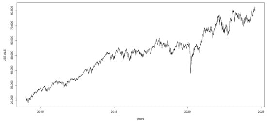
Figure 1.
Plot of the All-Share JSE stock index (2009–2025).
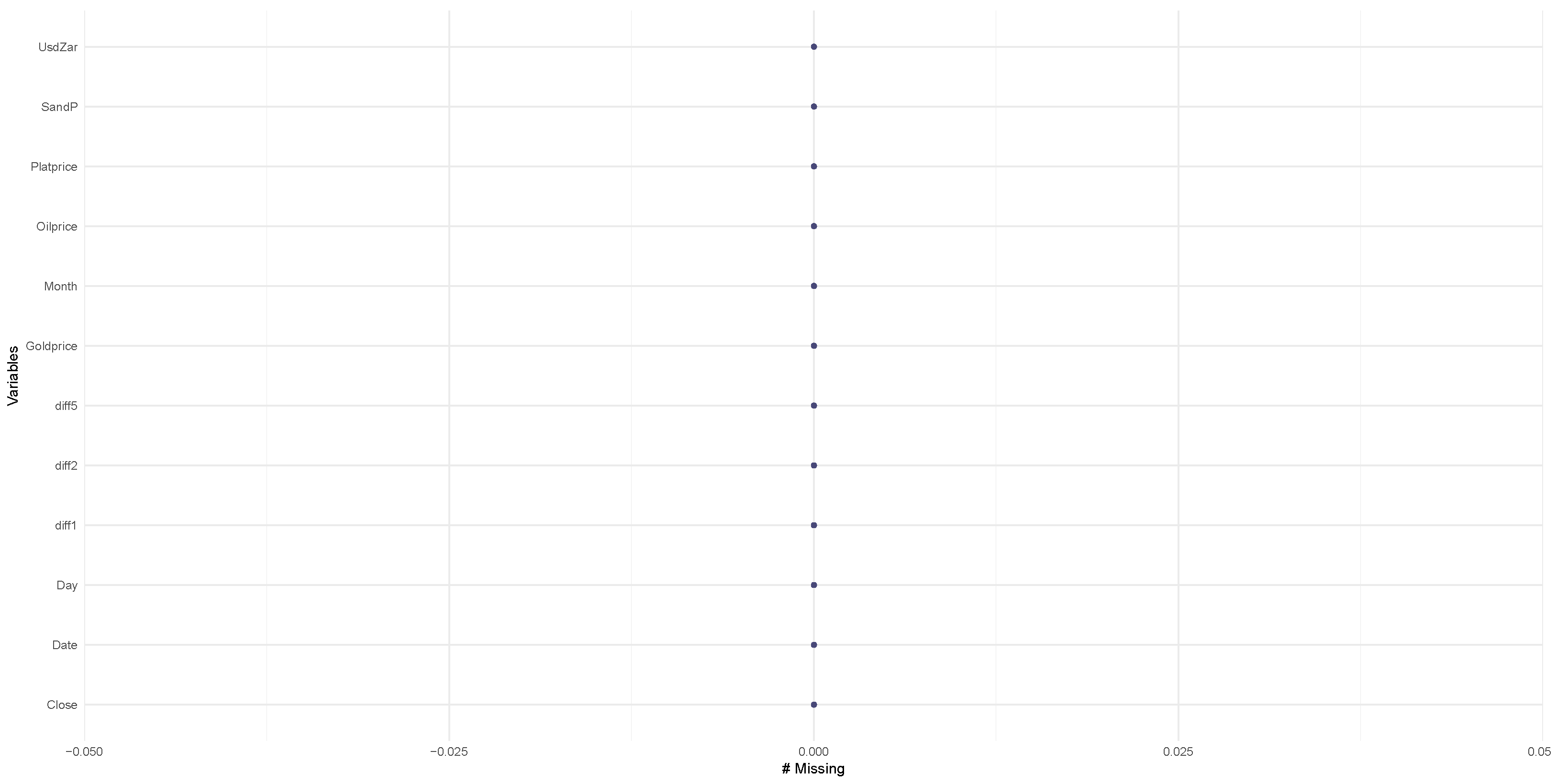
Figure 2 shows that the data has no missing values.
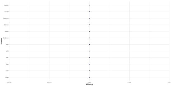
Figure 2.
Missing data plot.
3.3. Results
Variables Importance
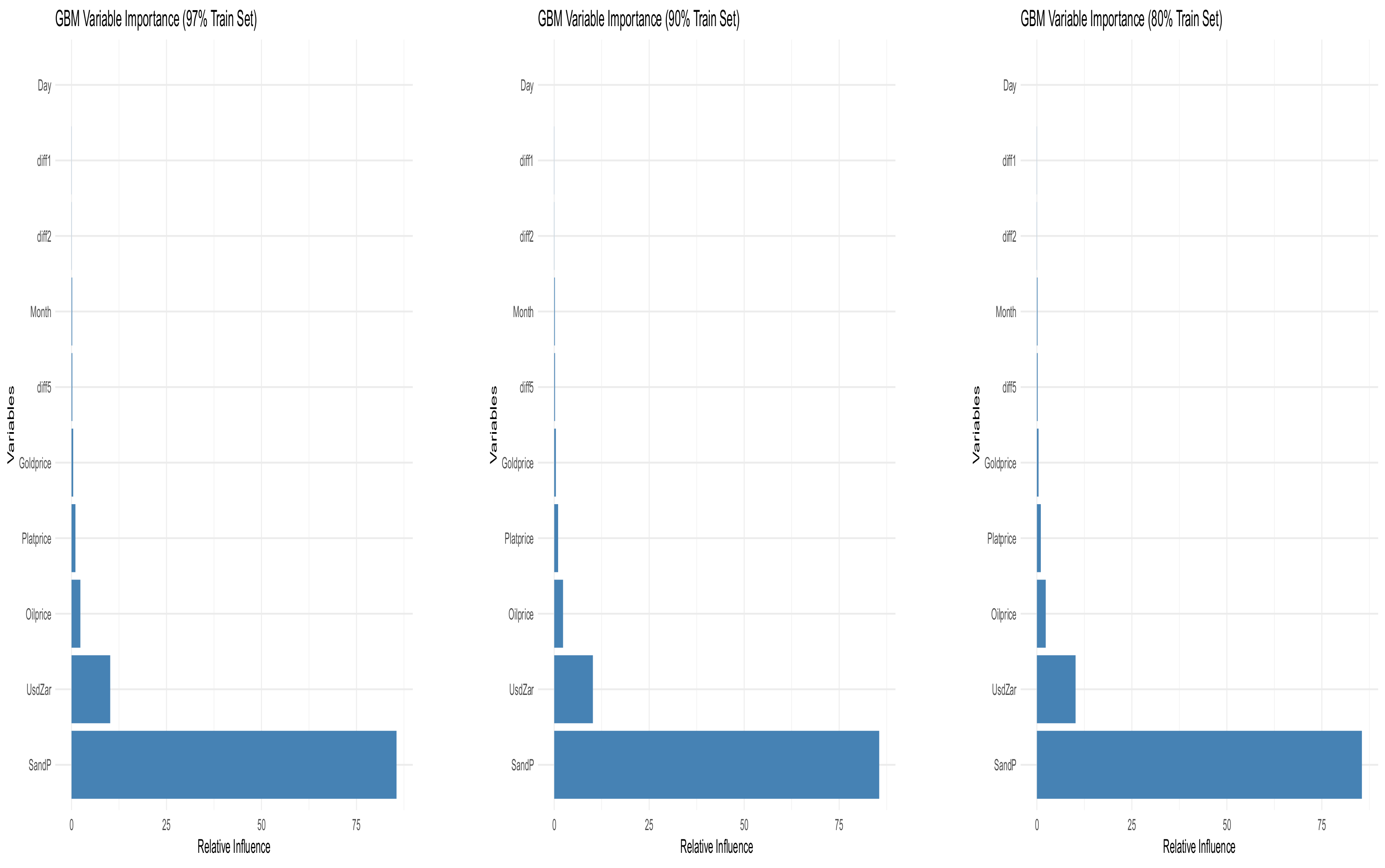
Figure 3 presents the graphical depiction of Table 2, Table 3 and Table 4, illustrating the relative influence of variables when training the Gradient Boosting Machine (GBM) model on 97%, 90%, and 80% of the data, respectively. Across all three training proportions, the SandP variable consistently shows the greatest influence, highlighting its dominant role in predicting the JSE All-Share Index. This is followed by UsdZar, Oilprice, Platprice, and Goldprice, which contribute meaningfully, though to a lesser extent. The lagged return features (diff5, diff2, and diff1) exhibit relatively low importance, while Month has minimal impact, and Day contributes nothing across all models. These findings emphasise that macroeconomic and international market indicators, particularly the S&P 500 index and USD/ZAR exchange rate, are critical predictors in forecasting the JSE ALSI, regardless of the training data size.
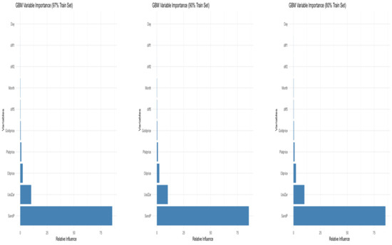
Figure 3.
Variable importance plots for GBM models trained using 97%, 90%, and 80% of the dataset, respectively. These plots illustrate how the contribution of each covariate varies depending on the size of the training set.
Table 2.
Variable importance using 97% of data set to train the GBM including external predictors (final update).
Table 3.
Variable importance using 90% of data set to train the GBM including external predictors (updated).
Table 4.
Variable importance using 80% of data set to train the GBM including external predictors.
Figure 3 displays the variable importance plots for GBM models trained on 97%, 90%, and 80% of the dataset. These plots highlight how each covariate’s influence changes with the training data’s size.
Table 5 presents the performance of the Gradient Boosting Machine (GBM) models evaluated using test set proportions of 3%, 10%, and 20%. All models were trained with identical hyperparameters: n.trees = 1000, interaction.depth = 4, shrinkage = 0.01, n.minobsinnode = 10, and cv.folds = 5. These settings were selected based on standard gradient boosting practices and further tuned empirically to achieve a balance between model complexity, regularisation, and generalisation. Among the three configurations, the 10% test set yielded the best performance, with the lowest values of MAE, RMSE, and MAPE, indicating strong predictive capability. In contrast, the 3% test split resulted in the poorest performance, including the highest RMSE and most pronounced negative bias, likely a consequence of overfitting due to insufficient validation data. The 20% test split performed slightly worse than the 10% split, possibly due to the smaller training set. Overall, the 90%/10% train/test split offered the most reliable and generalisable results.
Table 5.
Performance metrics of GBM models across different test set proportions using 5-fold cross-validation and 1000 trees.
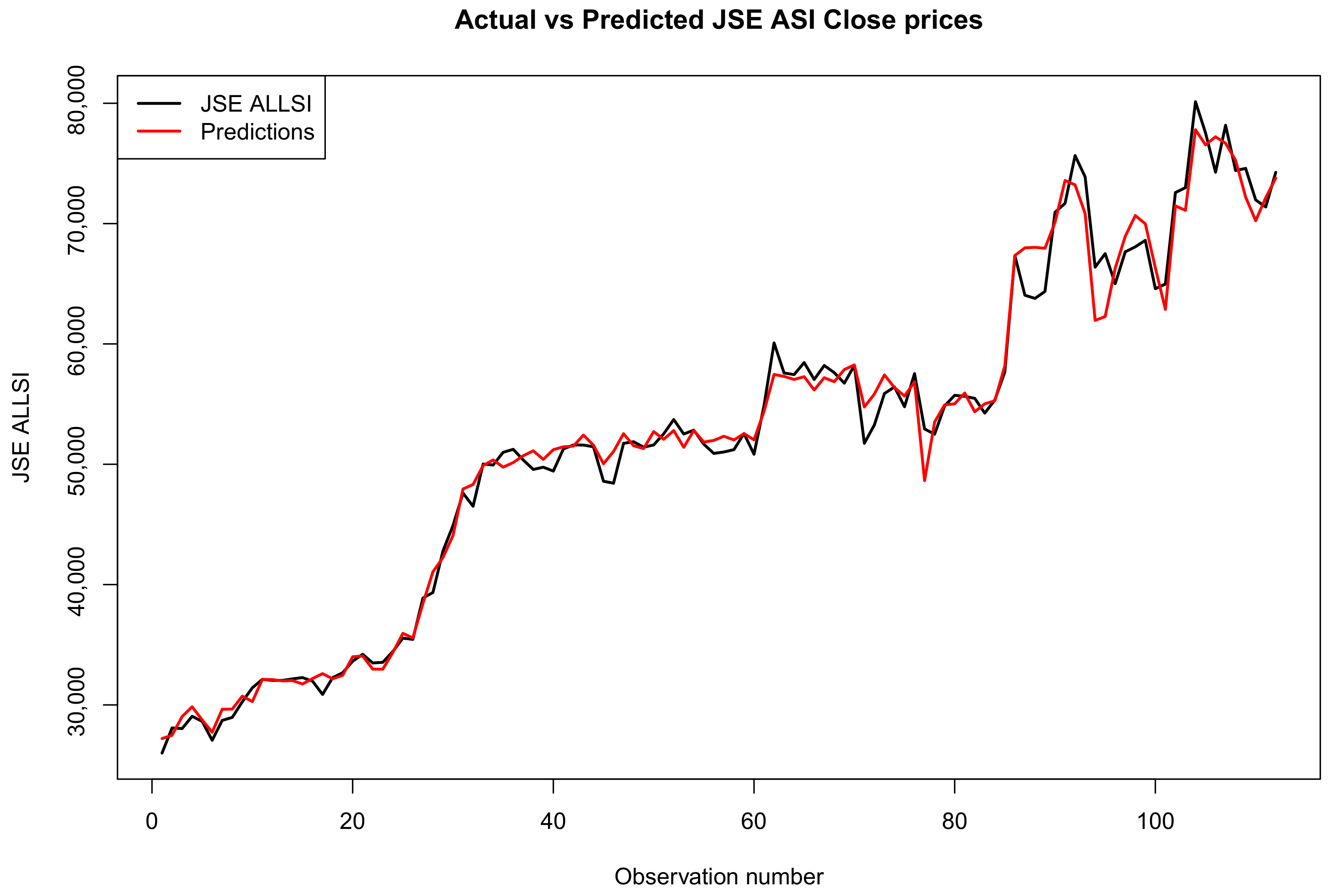
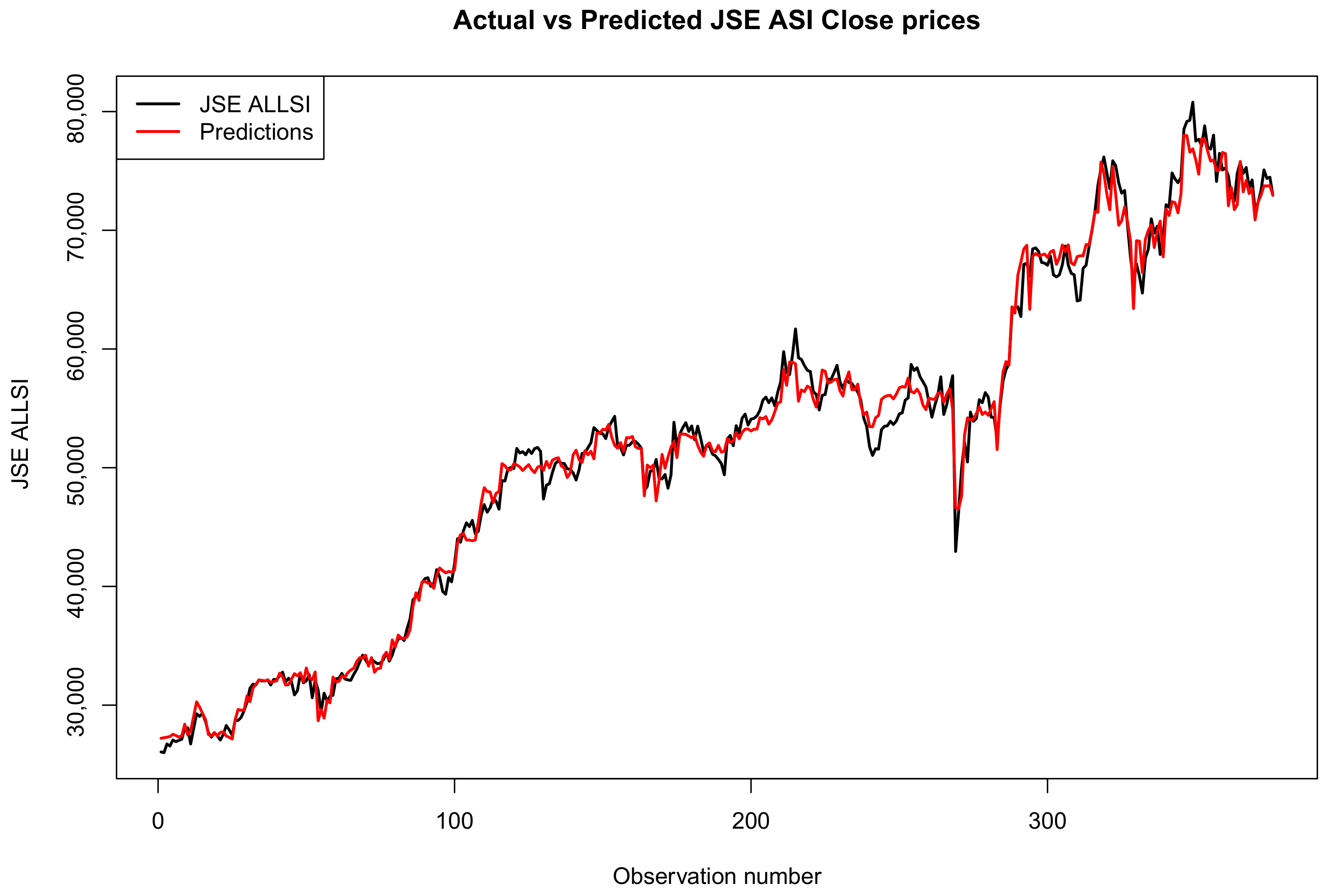
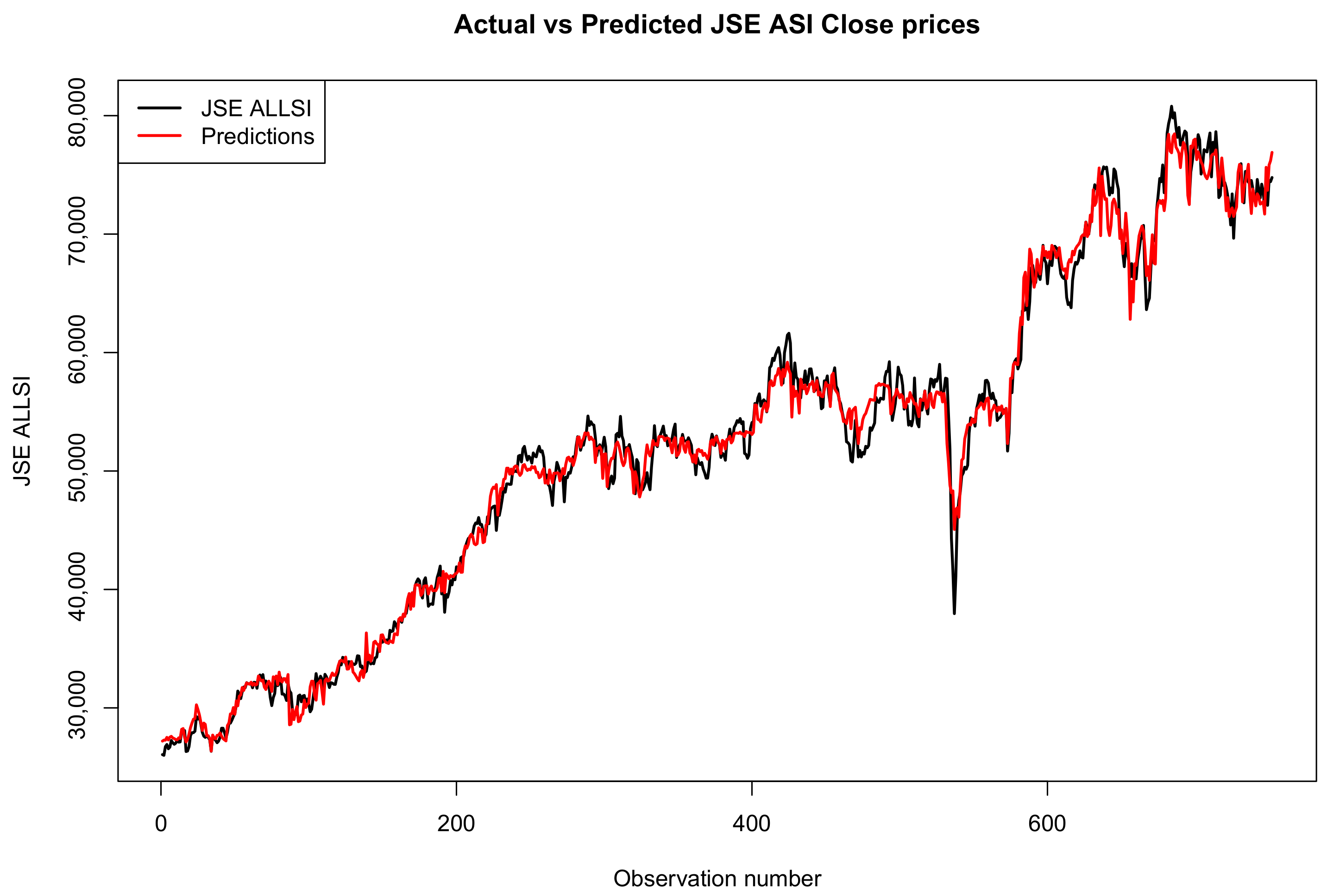
Figure 4, Figure 5 and Figure 6 show the comparison of actual and predicted JSE ALSI closing price values using 3%, 10% and 20% of the test data set, respectively.

Figure 4.
Comparison of actual and predicted JSE ALSI closing price values using 3% testing data.

Figure 5.
Comparison of actual and predicted JSE ALSI closing price values using 10% testing data.
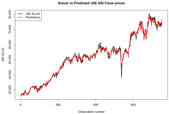
Figure 6.
Comparison of actual and predicted JSE ALSI closing price values using 20% testing data.
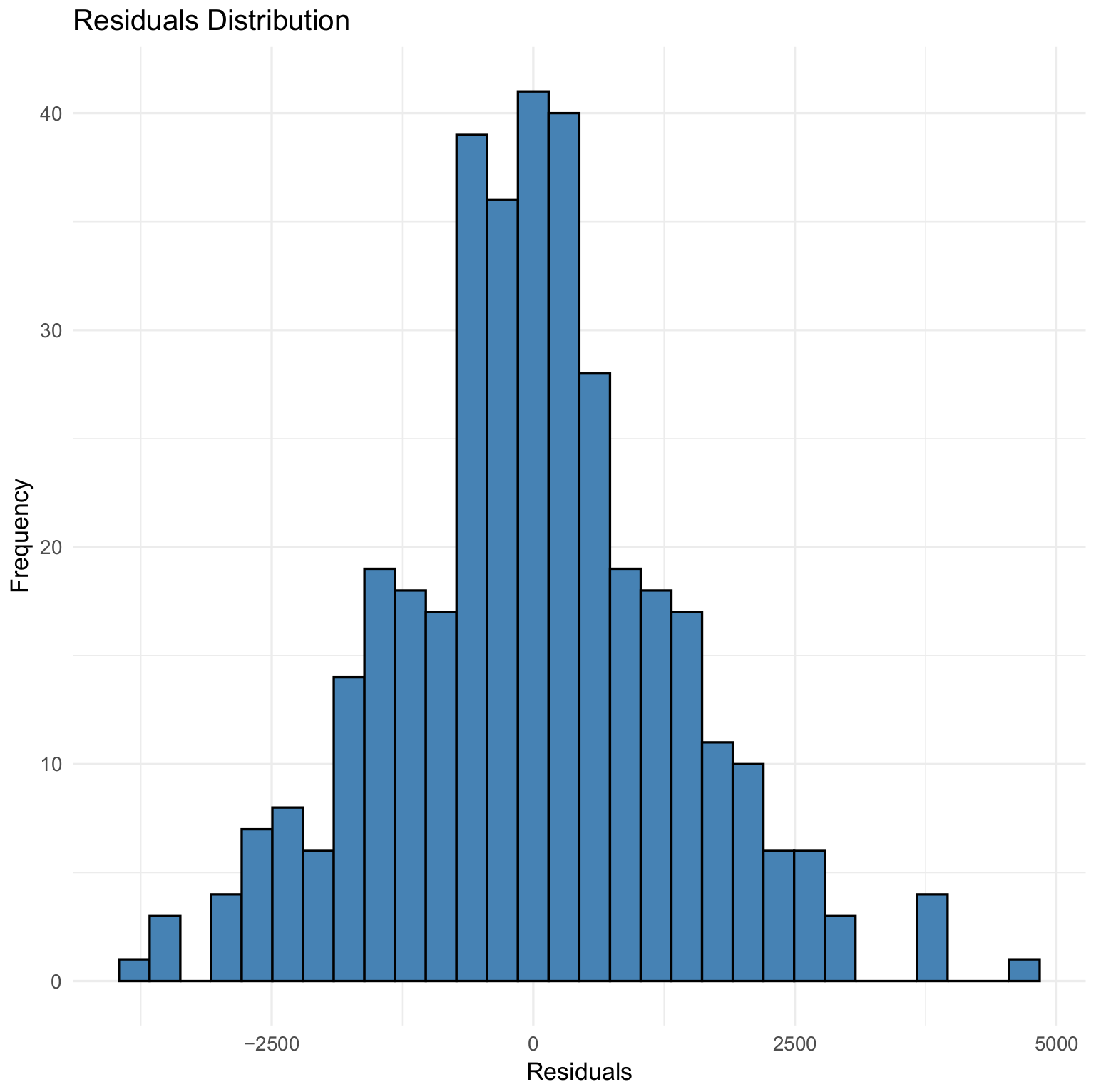
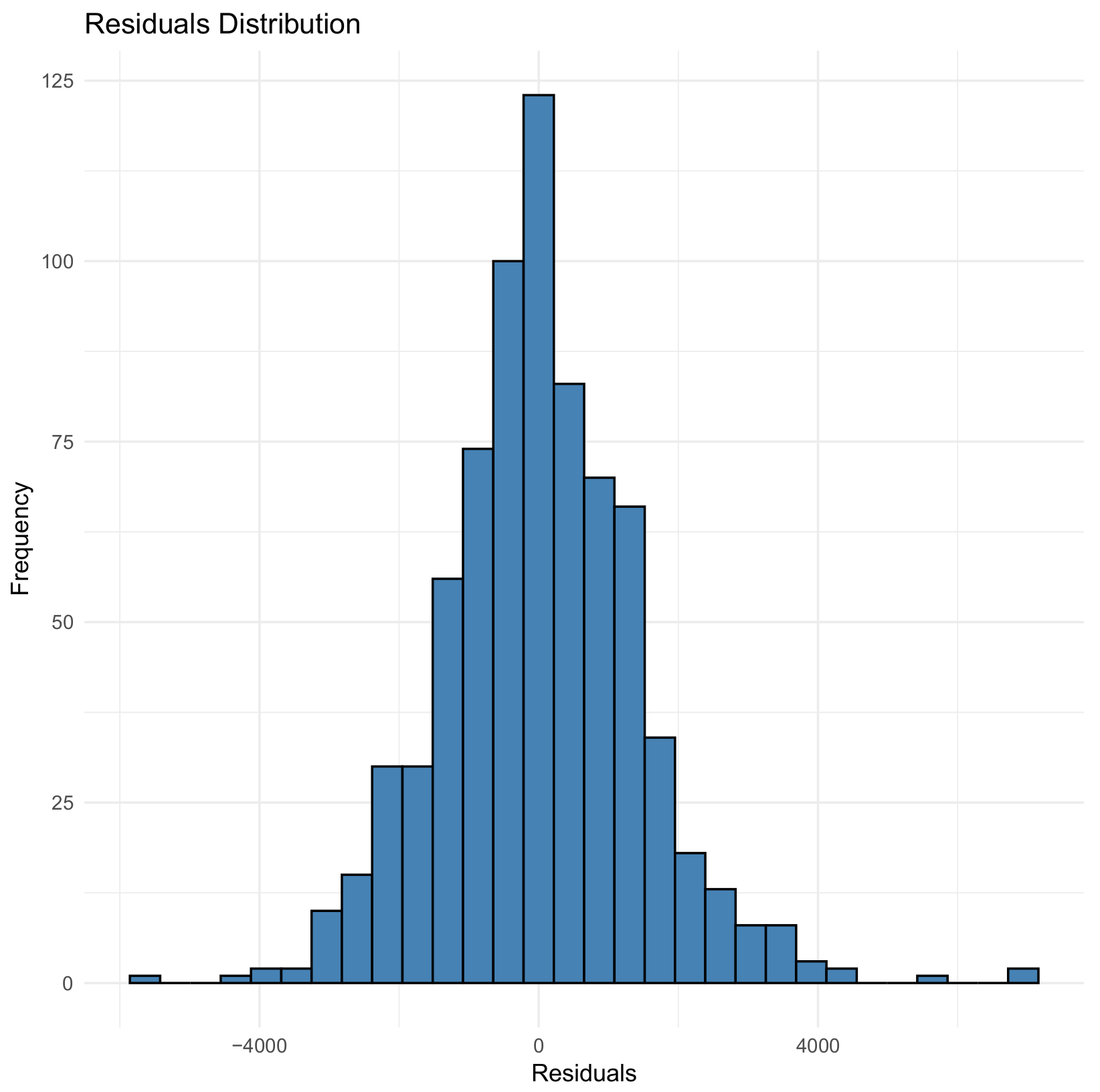
Figure 7, Figure 8 and Figure 9 illustrate the residual distributions for the 97%, 90%, and 80% validation sets, respectively, for the GBM model.
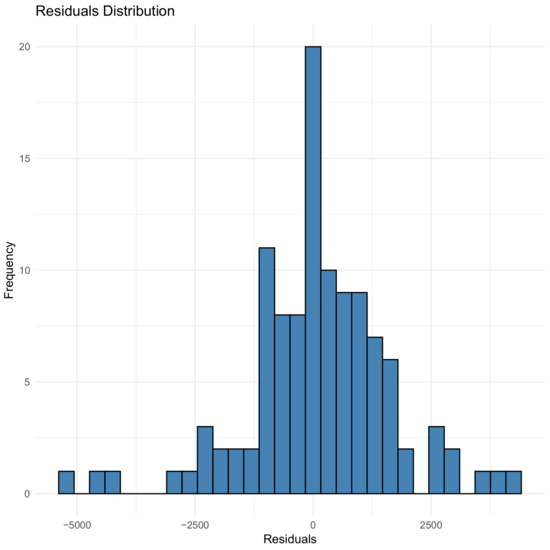
Figure 7.
Residual distribution for 97% validation for the GBM model.

Figure 8.
Residual distribution for 90% validation for the GBM model.
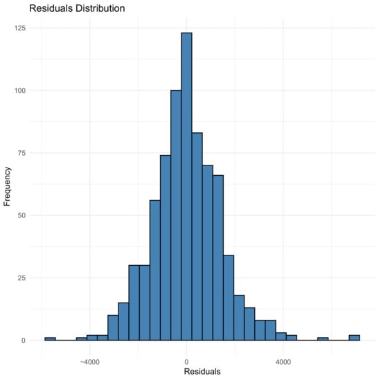
Figure 9.
Residual distribution for 80% validation for the GBM model.
3.4. Principal Component Regression
This is the benchmark model of this study.
Selection of Number of Components
In principal component regression (PCR), the covariates are first standardised by scaling them to have a mean and unit variance of zero. The transformation ensures that all variables contribute equally to the principal component analysis, preventing those with larger numerical ranges from dominating the resulting components.
The one-sigma heuristic was used to select the optimal number of components. According to Mevik and Wehrens (2015), the one-sigma heuristic involves selecting the model with the fewest components while remaining less than one standard error away from the overall best model. Let be the minimum cross-validated error obtained across all models, and let be the standard error associated with that minimum. The final number of principal components is then chosen as the smallest number k such that
This criterion ensures that the selected model is not only close in performance to the best model but also simpler, thereby reducing the risk of overfitting and improving generalisability.
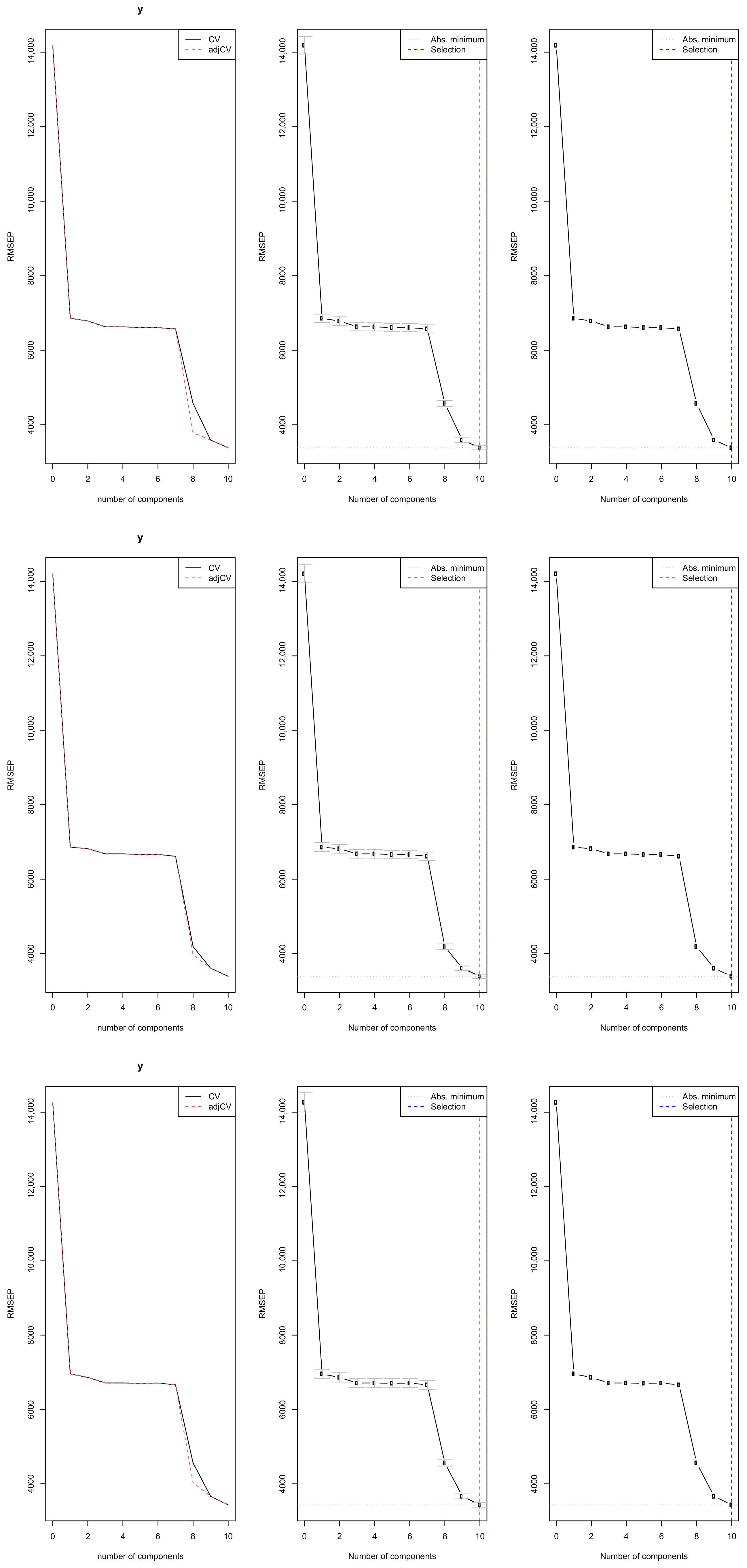
Figure 10 illustrates the optimal number of principal components selected by cross-validation for each training dataset. The results indicate that the PCR model requires 10 components to sufficiently explain the variation in the closing prices of the Johannesburg Stock Exchange All-Share Index across all splits. Using 10 components ensures that over 94% of the variance in the response variable (closing price) is explained, while the variance in the predictors (X) is fully captured as shown in Table 6. The cross-validation root mean square error of prediction (RMSEP) reaches its minimum at 10 components, indicating the best trade off between model complexity and predictive accuracy. This suggests that these 10 components capture the essential information from the explanatory variables needed for effective forecasting of the JSE ASI closing price.
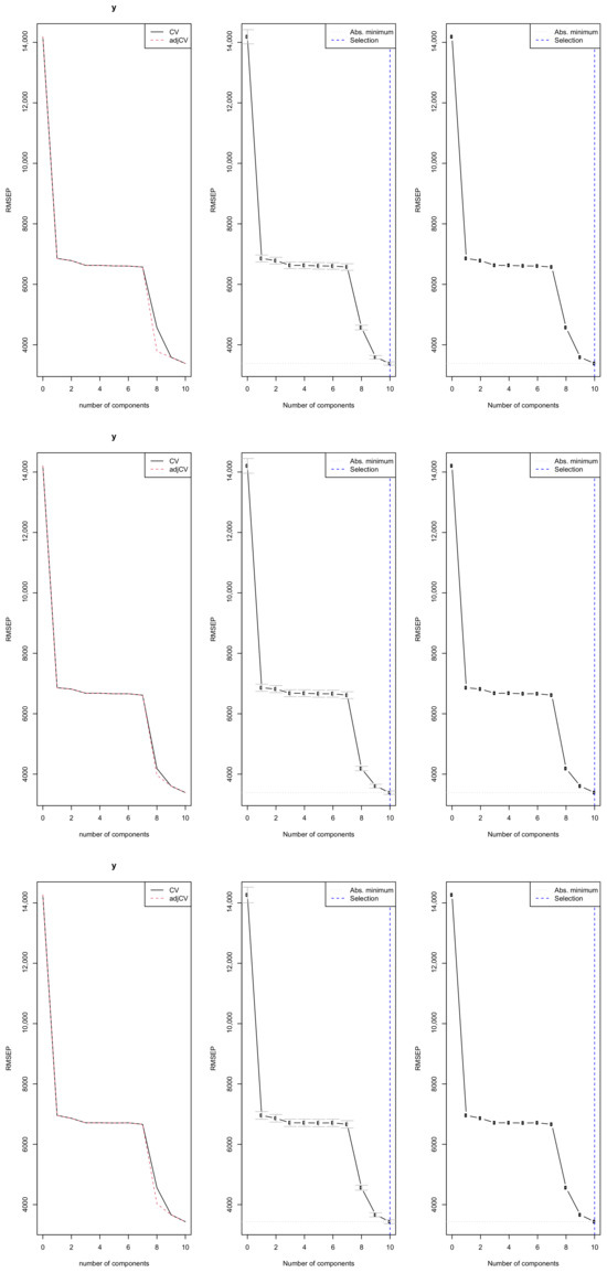
Figure 10.
PCR model selection: cross-validation RMSEP across components for three training splits 97%, 90%, and 80%, respectively.
Table 6.
PCR cross-validation RMSEP and variance explained (X and Y).
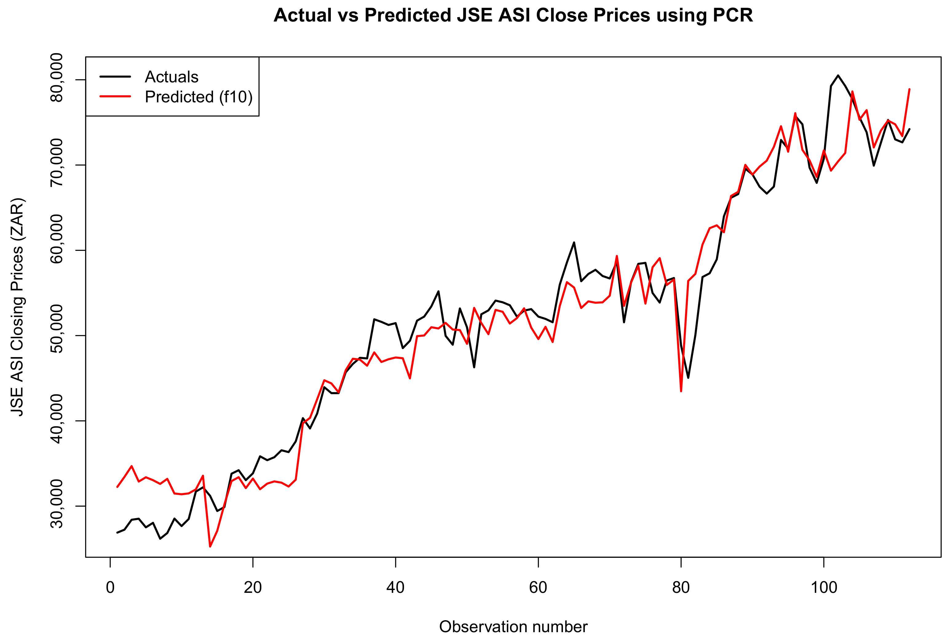
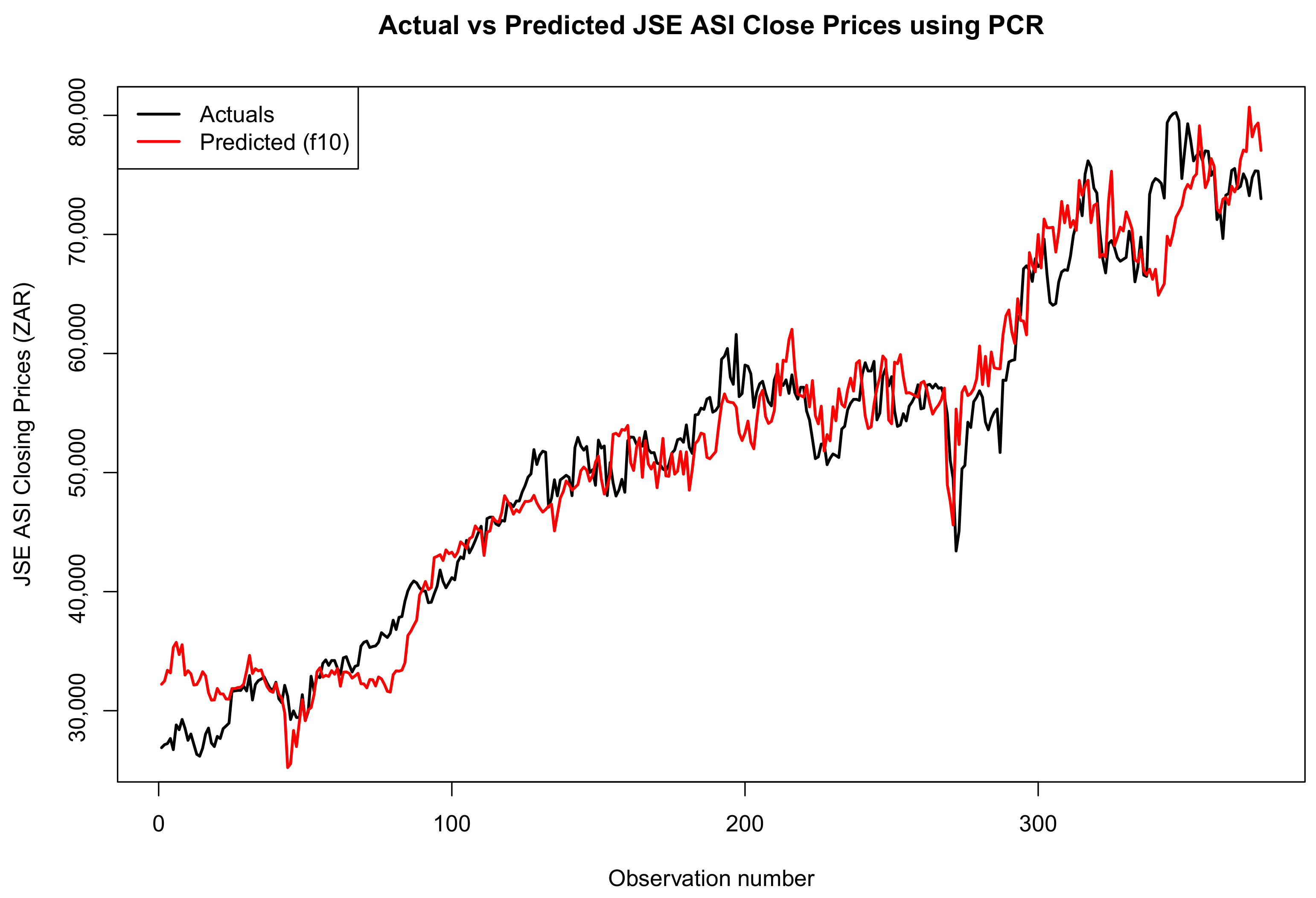
Figure 11, Figure 12 and Figure 13 show a comparison between the actual and predicted closing prices of the JSE ALSI index. These comparisons are based on the PCR model, using 3%, 10%, and 20% of the data for testing, respectively.
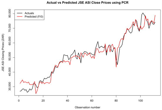
Figure 11.
Comparison of actual and predicted JSE ALSI closing price values using 3% testing data.

Figure 12.
Comparison of actual and predicted JSE ALSI closing price values using 10% testing data.
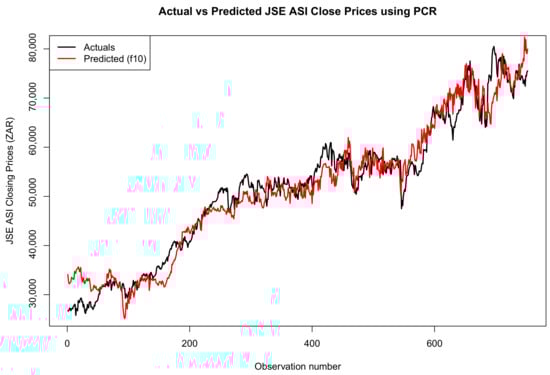
Figure 13.
Comparison of actual and predicted JSE ALSI closing price values using 20% testing data.
Table 7 presents the evaluation metrics, including bias, for the PCR model with 10 principal components across test sets of 20%, 10%, and 3%.
Table 7.
Evaluation metrics including bias for PCR model with 10 principal components across 20%, 10%, and 3% test sets.
3.5. Forecast Comparison of the Two Models
Forecast Accuracy
Table 8 presents a comparative analysis of the performance metrics for the GBM and PCR models across test set proportions of 3%, 10%, and 20%. The results clearly indicate that the GBM model consistently outperforms PCR across all evaluation metrics, including MAE, RMSE, MAPE, MASE, and Bias. Specifically, the GBM achieves significantly lower MAE and RMSE values at each split, suggesting that its predictions are closer to the true values compared to those of PCR. For instance, at the 10% test split, GBM records an MAE of 1029.34 and RMSE of 1343.93, whereas PCR records substantially higher values of 2663.51 and 3411.96, respectively. Similarly, GBM maintains lower MAPE values all below 0.021, while PCR’s MAPE remains above 0.054 across all test sizes, indicating weaker relative accuracy.
Table 8.
Comparison of performance metrics for the GBM and PCR models across different test set proportions. Both models were evaluated using 5-fold cross-validation. The GBM was trained with 1000 trees; PCR used 10 principal components.
In terms of forecasting efficiency, the GBM also demonstrates lower MASE values, with its best performance observed at the 3% test split 0.66410, while PCR’s MASE remains considerably higher, reaching 1.39911 at the same split. GBM shows minimal bias, particularly at the 10% split with a value of 22.41, reflecting well-calibrated predictions with little tendency to systematically over- or underpredict. In contrast, PCR exhibits notable bias, especially at the 3% test split, with a mean error of 108.63, and even higher discrepancies at larger splits.
Among the GBM configurations, the 10% test split delivers the best overall performance, achieving the lowest error and bias, suggesting that a 90/10 train/test ratio strikes the optimal balance between training data size and generalisation performance. Overall, the results demonstrate the superior predictive performance and robustness of the GBM model compared to PCR for short-term forecasting of the JSE ALSI. These findings highlight GBM’s consistency and reliability, particularly when evaluated using a 90/10 train/test split.
The results in Table 9 show the outcome of the Diebold–Mariano (DM) tests, which compare the predictive accuracy of two forecasting models, the GBM and PCR, for the JSE ASI closing prices under three different training/test splits. In all three scenarios, 97/3, 90/10, and 80/20 percent, the DM statistic is negative and highly significant with a p-value < 0.001, indicating that the GBM model consistently outperforms the PCR model in terms of forecasting accuracy. The negative DM values imply that the forecast errors of the GBM model are statistically smaller than those of the PCR model. The Significant label confirms that these differences are not due to random chance but reflect a meaningful performance gap between the models. This suggests that GBM is more effective for short-term forecasting of the JSE ASI, regardless of how the data is split for training and testing.
Table 9.
Comparison of GBM and PCR models on JSE ASI closing price forecasting across different training splits.
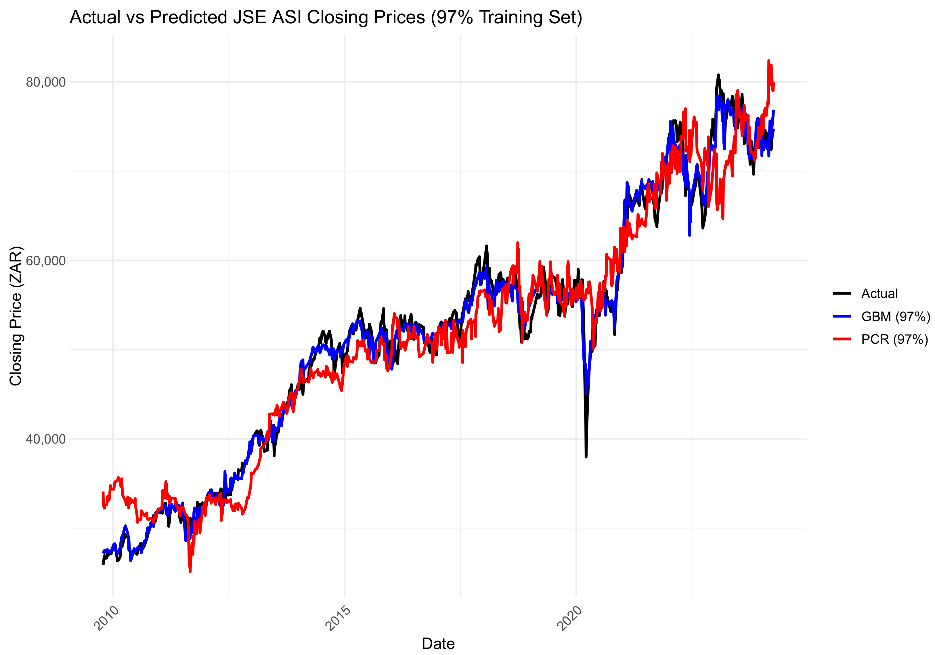
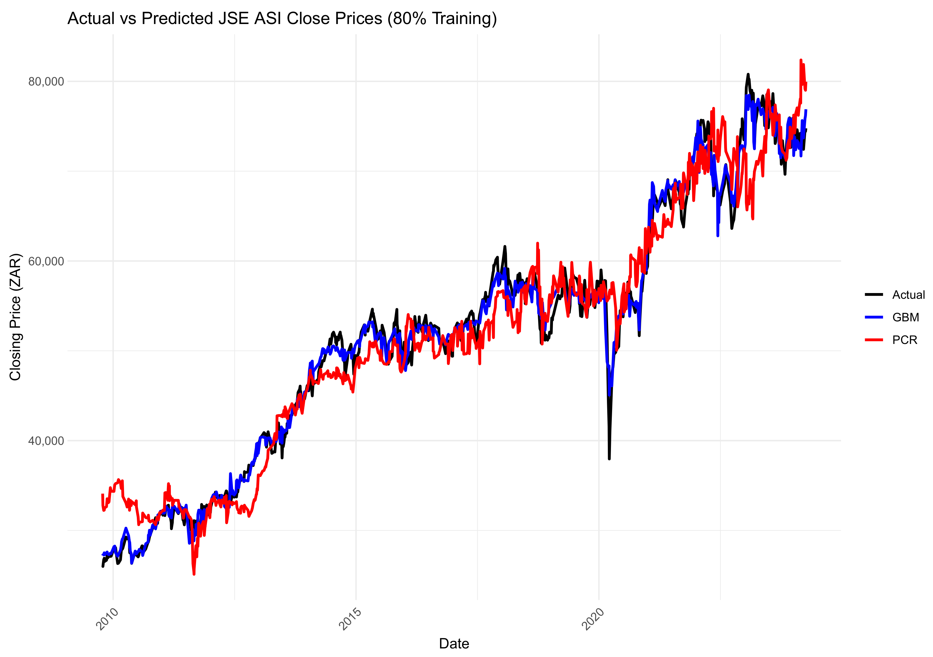
Figure 14, Figure 15 and Figure 16 compare the actual values, PCR predictions, and GBM predictions of the JSE ALSI closing prices using testing data proportions of 3%, 10%, and 20%, respectively.
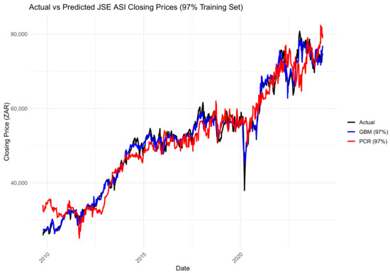
Figure 14.
Comparison of actual values, PCR predictions, and GBM predictions of JSE ALSI closing price values using 3% testing data.
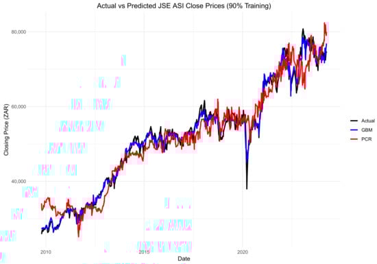
Figure 15.
Comparison of actual values, PCR predictions, and GBM predictions of the JSE ALSI closing price values using 10% testing data.
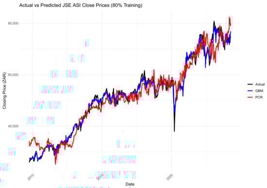
Figure 16.
Comparison of actual values, PCR predictions, and GBM predictions of JSE ALSI closing price values using 20% testing data.
4. Discussion
4.1. General Discussion
This study compared the short-term forecasting performance of the GBM and PCR for the JSE All-Share Index (ASI) closing prices. The analysis used three train–test splits: 97–3%, 90–10%, and 80–20%. Evaluation metrics included MAE, RMSE, MAPE, MASE, and the Diebold–Mariano (DM) test to assess the statistical significance of forecasting accuracy differences. Across all splits, the GBM consistently outperformed PCR, as indicated by significantly negative DM statistics and p-values below 0.001. These results suggest that the GBM’s forecasting errors were significantly lower than PCR’s, confirming the GBM’s superior predictive power for the JSE ASI data. This aligns with the broader literature, which frequently finds that ensemble learning methods like the GBM outperform traditional linear models in capturing the complexities of financial time-series data.
Notably, the performance gap between the GBM and PCR decreased slightly as the training set grew, particularly at the 97% split. This suggests that PCR’s performance becomes more competitive with larger datasets, but the GBM retains a clear advantage. The results also reflect the GBM’s ability to leverage nonlinearities and interactions in the data, especially in financial time series where complex dynamics often prevail.
While PCR remains a robust and interpretable method, particularly in small-sample or collinear settings, its linear structure limits adaptability to nonlinear patterns that the GBM captures well. The findings reinforce the importance of model flexibility and data-driven complexity when forecasting financial markets. The results also reinforce the prior literature affirming the GBM’s edge in short-term forecasting, particularly in contexts involving high-dimensional predictors and nonlinear relationships. Future research should explore whether combining PCR’s stability and the GBM’s flexibility through hybrid or ensemble methods can enhance forecasting accuracy, especially in varying market conditions or economic regimes.
4.2. Limitations of This Study
There are a few key limitations to this study. First, the comparison was limited to only two forecasting models: principal component regression (PCR) and one version of Gradient Boosting Machines (GBMs). This limited scope makes it difficult to generalise the findings, especially as other powerful models such as Random Forests, support vector machines, LSTM networks, and newer GBM variants such as XGBoost and LightGBM were excluded. Second, the GBM worked well, but the model was not substantially tuned. Only a fixed set of hyperparameters was utilised. A more extensive tuning technique may improve its performance. This study included three alternative training/testing splits. However, the test sets were relatively tiny, especially in the 90% and 97% training scenarios, which may have influenced the stability and repeatability of the performance measurements. Finally, while the GBM is effective at capturing complicated, nonlinear patterns, it has drawbacks: it is less interpretable, can be susceptible to outliers, and is prone to overfitting if not adequately regularised, particularly in financial time-series data, which frequently behaves unpredictably.
5. Conclusions
This research study predicts the JSE ASI Close price using the GBM Methodology with PCR as the benchmark method. The dataset used in this research study is the secondary data of the FTSE/JSE All-Share Index from 1 January 2009 to 8 August 2024. The freely accessible data is sourced from the website https://www.wsj.com/market-data/quotes/index/ZA/XJSE/ALSH/historical-prices (accessed on 7 October 2024). This data was processed using statistical analysis software R version 4.5.1 and RStudio version 2025.05.1-513 and the freely available R forecasting packages.
Table 8 shows that Gradient Boosting Machines (GBMs) outperform principal component regression (PCR) across all test set sizes in terms of predictive accuracy. The GBM consistently achieves lower MAE, RMSE, MAPE, and MASE values compared to PCR, indicating more accurate JSE All-Share Index forecasts. For example, with a 3% test set, GBM’s MAE is 1106.50 versus PCR’s 2551.56, and similar trends hold for RMSE and MAPE. This superior performance likely stems from the GBM’s strength in capturing complex nonlinear relationships and interactions in the data. In contrast, PCR’s higher errors suggest that while dimensionality reduction and feature extraction are useful, they may not fully capture the nonlinear patterns in this financial time series. Notably, the GBM’s bias values are closer to zero and more stable across test sizes, further supporting its robustness. Therefore, these results suggest that the GBM is better suited for forecasting the JSE All-Share Index under the current study conditions.
Future work should consider incorporating a broader set of relevant macroeconomic variables such as inflation rates, interest rates, and GDP growth to enhance forecasting accuracy potentially. While this study included important economic indicators like the USD/ZAR exchange rate, West Texas Intermediate (WTI) crude oil prices, platinum and gold international market prices, and the S&P 500 index, adding more macroeconomic factors could provide deeper insight into market dynamics. Additionally, temporal variables such as the month and day of the week were used here, but exploring more sophisticated time-related features or seasonal effects might further improve model performance. Moreover, investigating alternative or hybrid forecasting methods, including other machine learning algorithms and deep learning models, may offer a more comprehensive and nuanced understanding of the JSE All-Share Index’s short-term behaviour.
Author Contributions
Conceptualisation, M.M., T.R. and C.S.; methodology, M.M.; software, M.M.; validation, M.M., T.R. and C.S.; formal analysis, M.M.; investigation, M.M., T.R. and C.S.; data curation, M.M.; writing—original draft preparation, M.M.; writing—review and editing, M.M., T.R. and C.S.; visualisation, M.M.; supervision, T.R. and C.S.; project administration, T.R. and C.S.; funding acquisition, M.M. All authors have read and agreed to the published version of the manuscript.
Funding
This research was funded by the 2024 NRF Honours Postgraduate Scholarship: REF NO: PMDS230821144858.
Institutional Review Board Statement
Not applicable.
Informed Consent Statement
Not applicable.
Data Availability Statement
The data were obtained from the Wall Street Journal Markets website https://www.wsj.com/market-data/quotes/index/ZA/XJSE/ALSH/historical-prices (accessed on 7 October 2024), the FTSE/JSE Top 40 from https://za.investing.com/indices/ftse-jse-top-40-historical-data (accessed on 7 October 2024) and the S&P500 index data from https://www.wsj.com/market-data/quotes/index/SPX/historical-prices (accessed on 7 October 2024). The analytic data and data in brief can be accessed from https://github.com/csigauke/ (accessed on 7 October 2024).
Acknowledgments
The 2024 NRF Honours Postgraduate Scholarship support towards this research is hereby acknowledged. Opinions expressed and conclusions arrived at are those of the authors and are not necessarily to be attributed to the NRF. In addition, the authors thank the anonymous reviewers for their helpful comments on this paper.
Conflicts of Interest
The authors declare no conflicts of interest. The funders had no role in this study’s design; in the collection, analyses, or interpretation of data; in the writing of this manuscript; or in the decision to publish the results.
Abbreviations
The following abbreviations are used in this manuscript:
| ALSI | All-Share Index |
| ANN | Artificial Neural Network |
| CNN | Convolutional Neural Networs |
| DM | Diebold–Mariano |
| GBM | Gradient Boosting Machine |
| GAN | Genetic Adversarial Network |
| JSE | Johannesburg Stock Exchange |
| LSTM | Long Short-Term Memory |
| MAE | Mean Absolute Error |
| MAPE | Mean Absolute Percentage Error |
| MASE | Mean Absolute Scaled Error |
| PCA | Principal Component Analysis |
| RMSEP | Root Mean Square Error of Prediction |
| PCR | Principal Component Regression |
| RMSE | Root Mean Square Error |
| SVR | Support Vector Regression |
References
- Balusik, A., de Magalhaes, J., & Mbuvha, R. (2021). Forecasting the JSE top 40 using long short-term memory networks. arXiv, arXiv:2104.09855. [Google Scholar] [CrossRef]
- Breiman, L. (1996). Bagging predictors. Machine Learning, 24, 123–140. [Google Scholar] [CrossRef]
- Carte, D. (2009). The all-share index: Investing 101. Personal Finance, 2009(341), 9–10. Available online: https://hdl.handle.net/10520/EJC77651 (accessed on 13 June 2024).
- Castro, S. A. B. D., & Silva, A. C. (2024). Evaluation of PCA with variable selection for cluster typological domains. REM-International Engineering Journal, 77(2), e230071. [Google Scholar] [CrossRef]
- Chowdhury, M. S., Nabi, N., Rana, M. N. U., Shaima, M., Esa, H., Mitra, A., Mozumder, M. A. S., Liza, I. A., Sweet, M. M. R., & Naznin, R. (2024). Deep learning models for stock market forecasting: A comprehensive comparative analysis. Journal of Business and Management Studies, 6(2), 95–99. [Google Scholar] [CrossRef]
- Demirel, U., Çam, H., & Ünlü, R. (2021). Predicting stock prices using machine learning methods and deep learning algorithms: The sample of the istanbul stock exchange. Gazi University Journal of Science, 34(1), 63–82. [Google Scholar] [CrossRef]
- Dey, S., Kumar, Y., Saha, S., & Basak, S. (2016). Forecasting to classification: Predicting the direction of stock market price using Xtreme Gradient Boosting. PESIT South Campus, 1, 1–10. [Google Scholar] [CrossRef]
- El-Shal, A. M., & Ibrahim, M. M. (2020). Forecasting EGX 30 index using principal component regression and dimensionality reduction techniques. International Journal of Intelligent Computing and Information Sciences, 20(2), 1–10. [Google Scholar]
- Friedman, J. H. (2001). Greedy function approximation: A gradient boosting machine. Annals of Statistics, 29(5), 1189–1232. [Google Scholar] [CrossRef]
- Friedman, J. H. (2002). Stochastic gradient boosting. Computational Statistics & Data Analysis, 38(4), 367–378. [Google Scholar] [CrossRef]
- Green, A., & Romanov, E. (2024). The high-dimensional asymptotics of principal component regression. arXiv, arXiv:2405.11676. [Google Scholar] [CrossRef]
- Hargreaves, C. A., & Leran, C. (2020). Stock prediction using deep learning with long-short-term-memory networks. International Journal of Electronic Engineering and Computer Science, 5(3), 22–32. [Google Scholar]
- Kumar, D., Sarangi, P. K., & Verma, R. (2022). A systematic review of stock market prediction using machine learning and statistical techniques. Materials Today: Proceedings, 49, 3187–3191. [Google Scholar] [CrossRef]
- Kumar, G., Jain, S., & Singh, U. P. (2021). Stock market forecasting using computational intelligence: A survey. Archives of Computational Methods in Engineering, 28(3), 1069–1101. [Google Scholar] [CrossRef]
- Liu, R. X., Kuang, J., Gong, Q., & Hou, X. L. (2003). Principal component regression analysis with SPSS. Computer Methods and Programs in Biomedicine, 71(2), 141–147. [Google Scholar] [CrossRef] [PubMed]
- Mevik, B. H., & Wehrens, R. (2015). Introduction to the pls package. Help section of the “Pls” package of R studio software (pp. 1–23). Available online: https://cran.r-project.org/web/packages/pls/vignettes/pls-manual.pdf (accessed on 27 July 2025).
- Mokoaleli-Mokoteli, T., Ramsumar, S., & Vadapalli, H. (2019). The efficiency of ensemble classifiers in predicting the johannesburg stock exchange all-share index direction. Journal of Financial Management, Markets and Institutions, 7(02), 1950001. [Google Scholar] [CrossRef]
- Nabipour, M., Nayyeri, P., Jabani, H., Mosavi, A., & Salwana, E. (2020). Deep learning for stock market prediction. Entropy, 22(8), 840. [Google Scholar] [CrossRef]
- Natekin, A., & Knoll, A. (2013). Gradient boosting machines, a tutorial. Frontiers in Neurorobotics, 7, 21. [Google Scholar] [CrossRef]
- Nevasalmi, L. (2020). Forecasting multinomial stock returns using machine learning methods. The Journal of Finance and Data Science, 6, 86–106. [Google Scholar] [CrossRef]
- Olorunnimbe, K., & Viktor, H. (2023). Deep learning in the stock market—A systematic survey of practice, backtesting, and applications. Artificial Intelligence Review, 56, 2057–109. [Google Scholar] [CrossRef]
- Park, S., Jung, S., Lee, J., & Hur, J. (2023). A short-term forecasting of wind power outputs based on gradient boosting regression tree algorithms. Energies, 16(3), 1132. [Google Scholar] [CrossRef]
- Pashankar, S. S., Shendage, J. D., & Pawar, J. (2024). A comparative analysis of traditional and machine learning methods in forecasting the stock markets of China and the US. Forecasting, 4(1), 58–72. [Google Scholar] [CrossRef]
- Patel, J., Shah, S., Thakkar, P., & Kotecha, K. (2015). Predicting stock market index using a fusion of machine learning techniques. Expert Systems with Applications, 42(4), 2162–2172. [Google Scholar] [CrossRef]
- Peng, Y., & de Moraes Souza, J. G. (2024). Machine learning methods for financial forecasting and trading profitability: Evidence during the Russia–Ukraine war. Revista de Gestão, 31(2), 152–165. [Google Scholar] [CrossRef]
- Qin, Q., Wang, Q. G., Li, J., & Ge, S. S. (2013). Linear and non-linear trading models with gradient boosted random forests and application to Singapore stock market. Journal of Intelligent Learning Systems and Applications, 5(01), 1–10. [Google Scholar] [CrossRef]
- Quinlan, J. R. (1996). Bagging, boosting, and C4.5. AAAI/IAAI, 1, 725–730. [Google Scholar]
- Russell, F. T. S. E. (2017). FTSE/JSE all-share index. Health Care, 7(228,485), 3–50. [Google Scholar]
- Sadorsky, P. (2023). Machine learning techniques and data for stock market forecasting: A literature review. Expert Systems with Applications, 197, 116659. [Google Scholar] [CrossRef]
- Shen, J., & Shafiq, M. O. (2020). Short-term stock market price trend prediction using a comprehensive deep learning system. Journal of Big Data, 7, 1–33. [Google Scholar] [CrossRef]
- Shrivastav, L. K., & Kumar, R. (2022a). An ensemble of random forest gradient boosting machine and deep learning methods for stock price prediction. Journal of Information Technology Research (JITR), 15(1), 1–19. [Google Scholar] [CrossRef]
- Shrivastav, L. K., & Kumar, R. (2022b). Gradient boosting machine and deep learning approach in big data analysis: A case study of the stock market. Journal of Information Technology Research (JITR), 15(1), 1–20. [Google Scholar] [CrossRef]
- Soni, P., Tewari, Y., & Krishnan, D. (2022). Machine learning approaches in stock market prediction: A systematic review. Journal of Physics: Conference Series, 2161, 012065. [Google Scholar] [CrossRef]
- Thomas, J., Mayr, A., Bischl, B., Schmid, M., Smith, A., & Hofner, B. (2018). Gradient boosting for distributional regression: Faster tuning and improved variable selection via noncyclical updates. Statistics and Computing, 28, 673–687. [Google Scholar] [CrossRef]
- Vaisla, K. S., Bhatt, A. K., & Kumar, S. (2010). Stock market forecasting using artificial neural network and statistical technique: A comparison report. International Journal of Computer and Network Security, 2(8), 50–55. [Google Scholar]
- Yaroshchyk, P., Death, D. L., & Spencer, S. J. (2012). Comparison of principal components regression, partial least squares regression, multi-block partial least squares regression, and serial partial least squares regression algorithms for the analysis of Fe in iron ore using LIBS. Journal of Analytical Atomic Spectrometry, 27(1), 92–98. [Google Scholar] [CrossRef]


Disclaimer/Publisher’s Note: The statements, opinions and data contained in all publications are solely those of the individual author(s) and contributor(s) and not of MDPI and/or the editor(s). MDPI and/or the editor(s) disclaim responsibility for any injury to people or property resulting from any ideas, methods, instructions or products referred to in the content. |
© 2025 by the authors. Licensee MDPI, Basel, Switzerland. This article is an open access article distributed under the terms and conditions of the Creative Commons Attribution (CC BY) license (https://creativecommons.org/licenses/by/4.0/).