Abstract
This study explores how energy price inflation affects supply chain pressures under different levels of political uncertainty. Using local projection impulse–response functions, we examine the effects of oil price shocks under two regimes: one with above-average levels of political uncertainty and another with below-average uncertainty. While previous research has focused on the direct macroeconomic impacts of oil price shocks, particularly on firm costs and consumer prices, this study highlights the effects of these shocks on supply chain disruption as a whole. Our findings indicate that heightened political uncertainty significantly amplifies the impact of oil price shocks on supply chain pressures, causing notable and persistent disruptions. Conversely, when political stability is high, the response of supply chains to the same shocks is minimal, suggesting that a stable political environment fosters greater resilience in supply chains.
JEL Classification:
E32; Q43; Q48
1. Introduction and Motivational Model
Energy represents an integral component of most intermediate goods producers’ production functions. Consequently, volatility in energy markets that exacerbates energy costs can reverberate down production chains, putting upward pressure on supply chains and macroeconomic stability. As noted in the seminal work of Barsky and Kilian (2002), oil prices are not only responsible for many recessions in the history of the United States macroeconomy, but are also associated with periods of extreme inflation, lower levels of productivity, and consequently slower rates of economic growth. Reaffirmed in Engemann et al. (2011), it is a well-established stylized fact that oil shocks are a large driver of business cycle fluctuations, which in recent research is also closely linked to policy uncertainty shocks as per Fernández-Villaverde and Guerrón-Quintana (2020) and, more generally, supply chain volatility, or broader supply shocks (Gundersen, 2020).
Fundamentally, we ask ourselves how the degree of supply chain pressures is exacerbated by energy price inflation—or shocks—under two different regimes: regimes where political uncertainty deviates positively from the average level of uncertainty, and another where uncertainty deviates negatively away from the average level. This question is partially motivated by the wide-ranging literature concerning the broader macroeconomic impacts of oil price shocks on the aggregate economic supply of goods and services. In many ways, the direct impact of oil shocks can be felt in a firm’s costs, thereby reflecting higher consumer prices, among other consequences detrimental to household welfare. Indirectly, however, there is an argument to be made that global oil price shocks can add stress to value chains.
While global value chain disruption—and to a similar extent, oil price shocks—are exogenous, there is an argument to be made that policy responses can “cushion” some of the blow of these shocks, and reign in supply chain volatility or at the very least partially dampen the effects of supply chain disruptions felt by domestic industries and households. To understand the basic effects of oil price shocks, consider the following bivariate unrestricted vector autoregressive model (VAR) consisting of the following two endogenous variables: oil price inflation, , and supply chain disruption, . Equation (1) describes our reduced-form VAR.
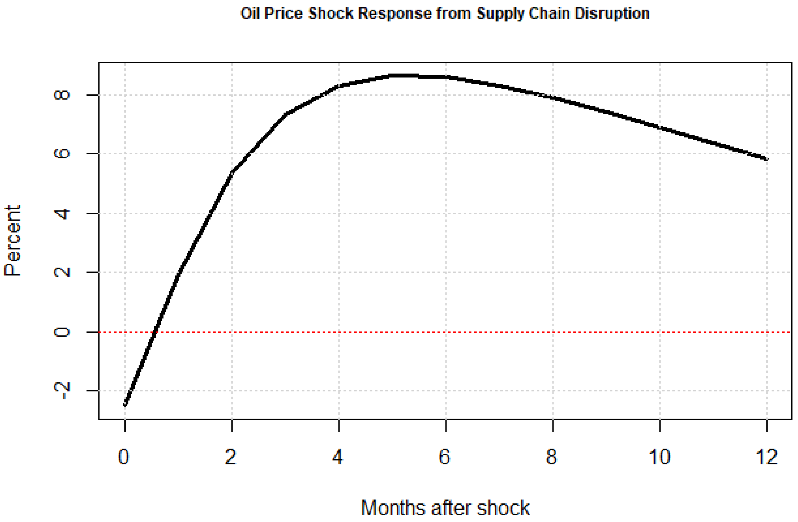
where is our vector of endogenous variables, is a drift term, and is a linear time trend. From Equation (1), we can simulate the response of a supply chain pressure to an oil price shock for months ahead. Figure 1 shows the results of this simulation.
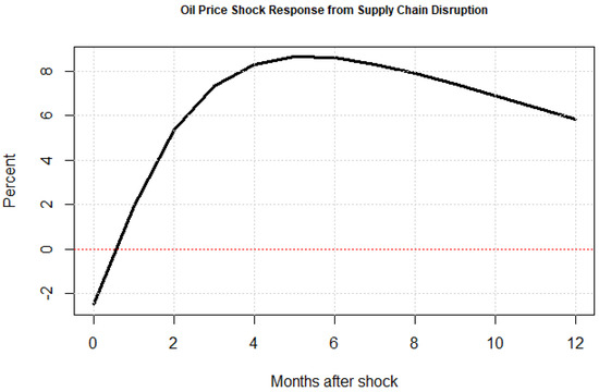
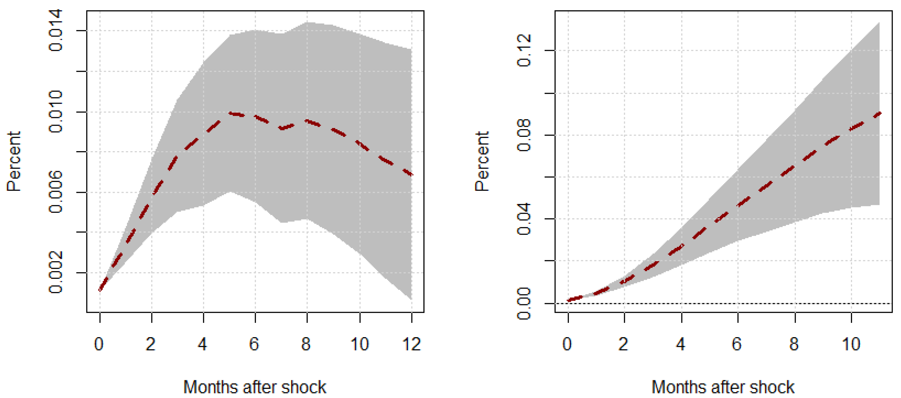
Figure 1.
Simple impact of oil price shocks on supply chain disruption. This figure shows the simple impact of a unit oil price shock on global supply chain pressure.
As is evident, at least visually speaking, we can see that the mean response of supply chain pressure to unit shock from oil price inflation elicits a peak response of around 8.5%, then tapering off to around 6%. Unsurprisingly, energy shocks or supply shocks, as captured by variations in oil price inflation, put considerable upward pressure on supply chains, pushing levels of disruption higher than the trend. The question then becomes, does policy—and subsequently, the stability of policy— dampen the effects of these shocks or exacerbate their magnitudes? To answer this question, we proceed with a brief review of the literature, discuss our principle data sources, perform econometric simulations, discuss our main results, and then conclude.
2. Literature
Our research lies at the intersection of a few distinct literature fields: oil (exogenous supply) shocks, supply chain disruption, and political uncertainty. While there are instances where two out of three of these distinct fields may overlap, there is very little work on the inter-relatedness of all three. Despite this, it stands to reason that both exist in the little literature, as well as the nature of our motivational model that exogenous oil supply shocks amplify supply chain volatility.
At the forefront of our field is the work of Barsky and Kilian (2002), Blanchard and Gali (2007), and Kilian et al. (2009). Notably, Barsky and Kilian (2002) analyze the relationship between oil price shocks and United States productivity, while complementary works like Nordhaus (2007) affirm the general proposition of oil price shocks as a form of an economic contraction in nature. The authors also argue that oil price shocks are a proxy for shocks to energy in general. In the representative firm’s production function, energy price shocks are generally seen as a negative shock to the production frontier the firm faces, thereby reducing aggregate productivity. While Barsky and Kilian (2002) link newer eras of oil price shocks to the declines in productivity and increases in the rate of inflation, the authors also challenge the notion that oil price shocks are strictly exogenous. In point of fact, the authors find that exogenous political events, along with other key macroeconomic variables, also play a central role in modeling the oil market and describing oil price shocks.
In many ways, this work opens up the possibility that political uncertainty can play a role in helping or hindering the response of key macroeconomic factors to oil price shocks. More recently, works like Kang et al. (2017) are at the intersection of oil price shocks with political uncertainty and economic security, and find that oil price shocks are positively linked to political uncertainty. Furthermore, the authors quantify the relative volatility in consumer price inflation, as explained by oil price shocks to be around 21%, further reinforcing the strain that such shocks can have on macroeconomic welfare. Similarly, Jiménez-Rodríguez (2022) studies the response of global economic activity in response to oil price shocks using a time-varying VAR model. The authors find that unexpected shocks cause a large, and persistent decline in global economic activity, which is not inconsistent with our main results in that policy uncertainty can exacerbate the degree to which oil price shocks inflate supply chain disruption.
Delving deeper into the literature on political uncertainty, Fernández-Villaverde and Guerrón-Quintana (2020) reviews the literature examining the relationship between political uncertainty and the business cycle, ascribing part of the business cycle to variation in the levels of political uncertainty. The authors note that uncertainty tends to run counter to the business cycle, which is to say that periods of higher political uncertainty are correlated with periods of lower real economic activity. The authors also note that causal direction is not well-established between the political cycle and business cycle—while out of scope, this is perhaps an avenue for extending our study and the broader literature. Herrera et al. (2019) further stress the importance of news and political uncertainty as key factors that influence the responsiveness of the broader macroeconomy to oil price shocks.
On a related note, both Bekiros et al. (2015) and Balcilar et al. (2017) recognize the significance of political stability as inherent to oil market returns and demand and estimate the degree to which news-based policy and economic uncertainty play a role in oil market predictability. To this end, these authors take a more rigorous and complex approach toward a nonparametric estimation of the volatility of oil market returns, taking into consideration the nonlinearities associated with the uncertainty measures of interest in their respective studies.
Finally, oil prices can also be thought of as a form of commodity price shocks. As such, there is one field that views energy or oil shocks through the lens of commodity price volatility. Of note in this literature field is Diaz et al. (2023), who analyzes the impacts of commodity price shocks on supply pressure and the subsequent pass-through of commodity price shocks to United States consumer price inflation. Using a structural VAR (SVAR) model, the authors construct time-varying impulse–response functions. The authors determine that much of the variation in both magnitude and significance of cost–push commodity price shocks occurred mostly over the past two decades, with extreme stress over the COVID-19 pandemic in particular. Similarly, (Gundersen, 2020) argue that the United States is more sensitive to supply shocks or price shocks in comparison to other nations, in part due to technological frictions that the United States is uniquely exposed to downstream.
While fewer and farther between, there is some work looking at political uncertainty in the context of its impact on supply chain resilience. Take, for instance, Odulaja et al. (2023), who conduct a thorough literature review examining the vulnerability of global value chains to geopolitical uncertainty. The authors find that, at a microeconomic level, value chains are generally less resilient in the face of rising political uncertainty due to factors like a lack of diversification from upstream members of the value chain and technological stagnation. Similarly, Nitsche and Durach (2018) also expands on the literature on supply chain volatility, considering political uncertainty to be a key macroeconomic factor inducing volatility across value chains. Looking at the intersection of supply chain disruptions and oil price shocks, Acemoglu and Tahbaz-Salehi (2024) studies the implications of supply chain disruptions as they relate to aggregate productivity. The authors find that even small shocks can lead to discontinuous changes in output even if efficient allocation remains continuous. Our results show that some of these discontinuities could be attributable to policy uncertainty. More broadly, there are some smaller literature reviews, like Baldwin and Freeman (2022), which stress the relationship between policy agendas and policy uncertainty, as such concepts relate to the severity of supply chain disruptions.
In essence, there is a myriad of related works of literature that examine the intersection of oil price shocks and political uncertainty, oil price shocks, supply chain stress, and subsequently, productivity, as well as a smaller subset looking at the intersection of supply chain volatility and energy price shocks. We contribute to the union of these distinct literature sets by considering the possibility that political uncertainty is akin to an environmental factor that broadly affects supply chain pressures or conditions, and subsequent responses of supply chain stresses to exogenous oil shocks.
3. Data
Given that we ultimately wish to identify periods of time where political uncertainty is higher than the trend and periods where uncertainty is lower, prior to econometric analysis, we will first need to detrend and extract the cyclical component of the political uncertainty index. Following this exercise, we then report descriptive statistics on the remaining data essential for our econometric analysis alongside any necessary transformations of the data.
3.1. Extracting Policy Cycles
To begin extracting policy cycles, consider the possibility that the level of political uncertainty, , can be decomposed such that:
where is an oscillatory (or cyclical) component of , while is the trend component. Assume oscillates between a lower bound, , and upper bound, , where the following inequality holds: . The power of the component only occurs over the interval such that and . As in sample size, the following bandpass filter can be utilized to approximate the cyclical component, :
where is our lag operator. Equation (3) can be expressed more extensively as Equation (4).
The optimal bandpass filter weights are defined by equation array (5).
Using the Hodrick and Prescott (1997) filter obtains the optimal filter weights via the following minimization problem described by (6).
which can be further approximated with finite data series as a series of moving average weights described by Equation (7).
where our empirical smoothing parameter, , is set to 129,600 given the monthly frequency of our data as per Ravn and Uhlig (2002). The result of our decomposition efforts produces Figure 2.
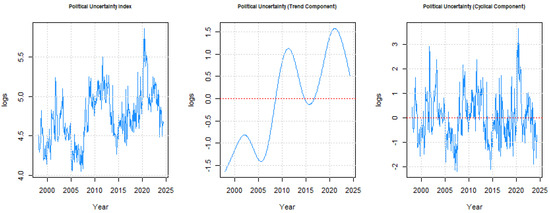
Figure 2.
Political uncertainty index decomposition. This figure shows our political uncertainty index, (left panel), the demeaned trend component, (middle), and our demeaned cyclical component, (right panel).
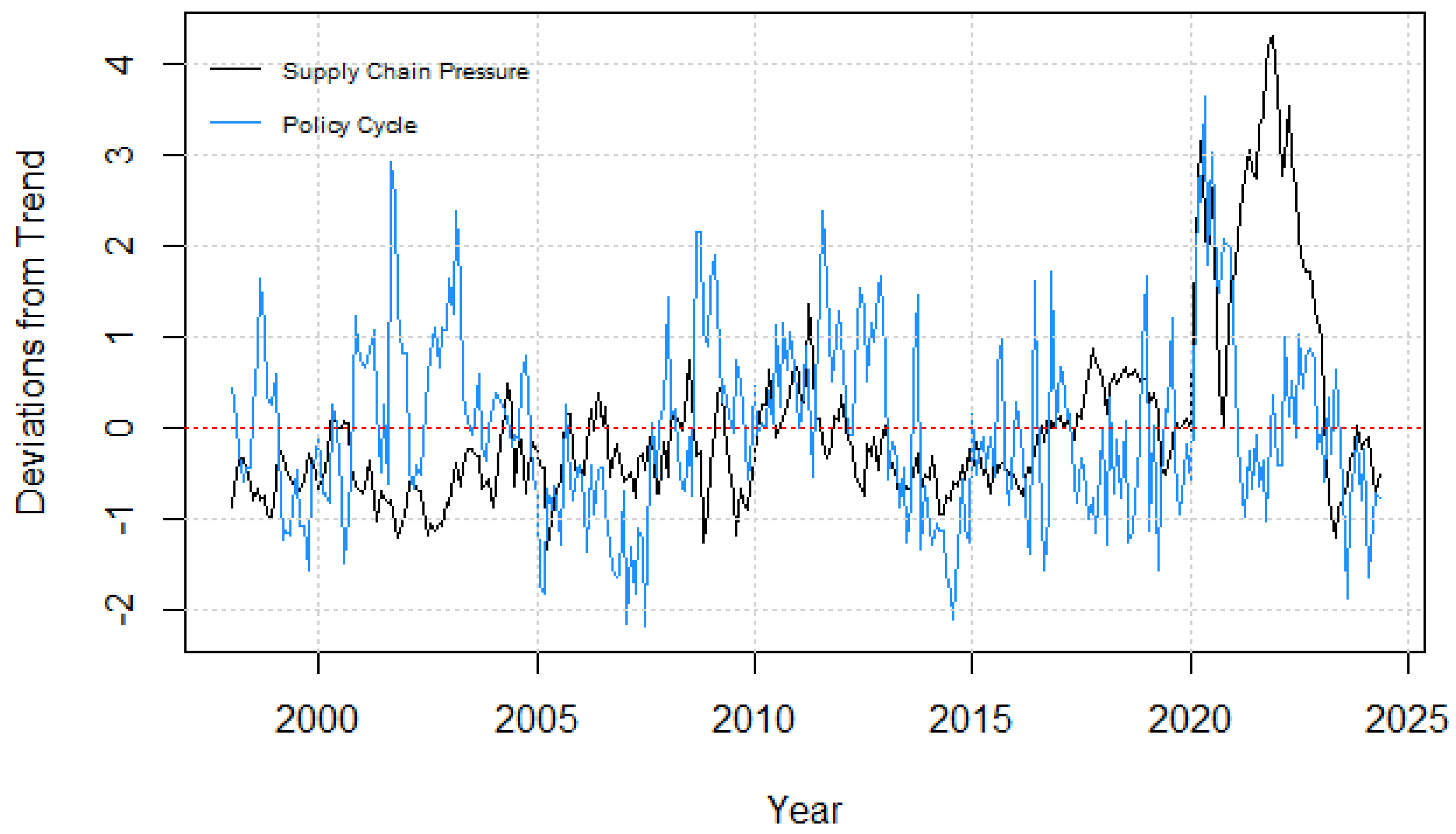
The right-most panel of Figure 3 shows the cyclical component of our logged and demeaned political uncertainty index. Much like the supply chain pressure index, we interpret our political cycle component as log deviations from the trend. When comparing both the supply chain pressure index to our political cycle index, we can see, via Figure 3, that both series tend to move mostly opposite to one another over time.
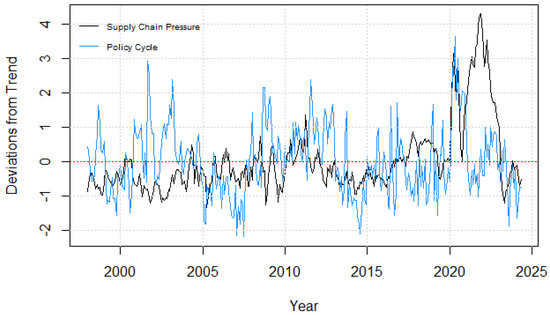
Figure 3.
Comparing supply chain pressures and political cycles. This figure simultaneously shows the supply chain pressure index plotted against the political cycle data, .
Figure 3 illustrates that over some periods, it tends to be the case that both supply chain pressures and political cycles move in tandem; however, there are periods where they move opposite of one another, suggesting political pressures play a role in dampening or exacerbating supply chain pressures but, at times, have little impact at all. As such, we pursue an empirical strategy that considers the possibility that political cycle stability is regime-specific; therefore, any shocks that crude oil prices may have on supply chain pressures are state-dependent.
3.2. Descriptive Statistics
All data are from the United States and span from January 1998 through May 2024, making for a sample size of . The level of political uncertainty in the United States is pulled from the Economic Policy Uncertainty database, while crude oil prices are reported at daily frequencies, and subsequently averaged to monthly frequencies by the U.S. Energy Administration.1 Finally, data on global supply chain pressures are available from the New York Fed. With our policy uncertainty cycle derived in Section 3.1, , we convert the crude oil price level to a rate of inflation by taking the log of the ratio of crude oil prices at time t relative to months ago, such that . While unreported, we utilize augmented Dickey–Fuller tests to ensure and subsequently confirm that our data are stationary and suitable for further econometric analysis. Table 1 reports descriptive statistics and correlation coefficients associated with our principle data series.

Table 1.
Descriptive statistics. These data show descriptive statistics and correlation coefficients for each of our principle data series spanning from January 1998 through May 2024.
We note that there is a characteristically positive correlation between supply chain pressure and oil price inflation, while there is an inverse relationship between oil price inflation and policy uncertainty. We also note that both supply chain pressure and policy uncertainty are equally volatile and higher in magnitude in their extreme values in comparison to oil price inflation. As such, we should expect some rigidity in the response of oil price inflation to shocks of either supply chain pressure or policy uncertainty.
4. Econometric Analysis
Given that we take the perspective that political uncertainty is a regime-switching environmental factor, it stands to reason that oil supply shocks will be conditional on the state of political uncertainty. As such, we adopt the Jordà (2005) local project impulse–response function approach for evaluating the asymmetries in responses of global supply chain pressure to oil price shocks in the United States. We opt for this simulation method for several reasons: firstly, local project impulse–response functions offer a much richer level of analysis compared to traditional linear VAR methods; secondly, such local methods tend to be more robust to model misspecification; finally, we aim to keep our model as parsimonious as possible, thus local project models of the variety described in Jordà (2005) not only capture complex nonlinearities in the data generating processes we examine but do so in the most tractable way possible.
Beyond the low-cost nature of local projection approaches, they are also incredibly convenient for capturing the effects of regime-switching variables, as they permeate through other key macroeconomic shocks. Specific to our study, we are not directly testing for the effects of political cycle volatility on supply chain pressure; rather, we are interested in how political cycle volatility can influence oil price shocks, which in turn affect supply chain stress. In essence, our study is keen on isolating the effects of oil price shocks on supply chain duress, with political cycle volatility having a direct impact on oil price pressures and an indirect effect on supply chain pressure.
The nature of our study’s research design is strictly more compatible with local projection methods than alternatives like a smooth transition vector autoregressive model or a threshold vector autoregressive model, specifically because we are not interested in testing the nonlinear impacts of political cycle volatility on supply chain pressure itself but rather the impacts of political uncertainty on energy price shocks which elicit a linear response from supply chain pressure.
Local Projection Impulse–Response Functions
Recall that at the outset, our motivating question is whether or not the volatility of political uncertainty can help or hinder the degree to which oil supply shocks exacerbate supply chain disruption. Given that political uncertainty has a strong cyclical component, as per Figure 2, we consider the possibility that two possible regimes exist, , and , respectively, where:
In essence, there is a world where political uncertainty fluctuates above the trend and a world where political uncertainty is at or below the trend level of uncertainty. With these regimes in mind, we can leverage the methodology described in Jordà (2005) to simulate the responses of supply chain pressures to unit oil supply shocks under state dependence. Formally, our local projection model takes on the following general form described by Equation (9).
where describes our vector of endogenous variables, h describes our forecast horizon, describes our lag length, as selected by the AIC criteria, and describes our lagged coefficient vectors corresponding to lag i and regimes . Furthermore, our state probabilities are computed via a logistic function that follows the form of Equation (10).
where describes our time-invariant scaling factor. With our model definitions in mind, we can compute state-dependent nonlinear impulse–response functions described by Equation (11).
Where captures our states such that , h captures our forecast horizon, and is a matrix of our shocks.2 Figure 4 illustrates the responses of supply chain pressure to a unit oil price shock under the regime where political uncertainty is strictly greater than the trend level of uncertainty or . Similarly, Figure 5 shows the responses of supply chain pressure to a unit oil price shock under the regime where political uncertainty is less than or equal to the trend level of uncertainty, or .
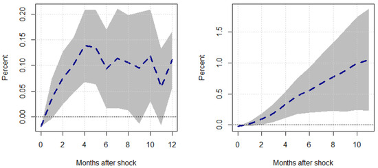
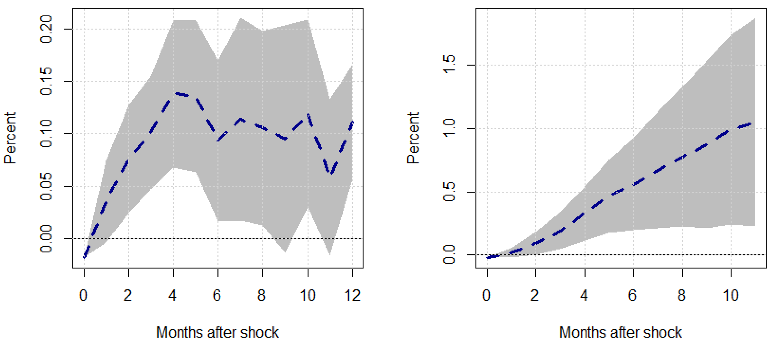
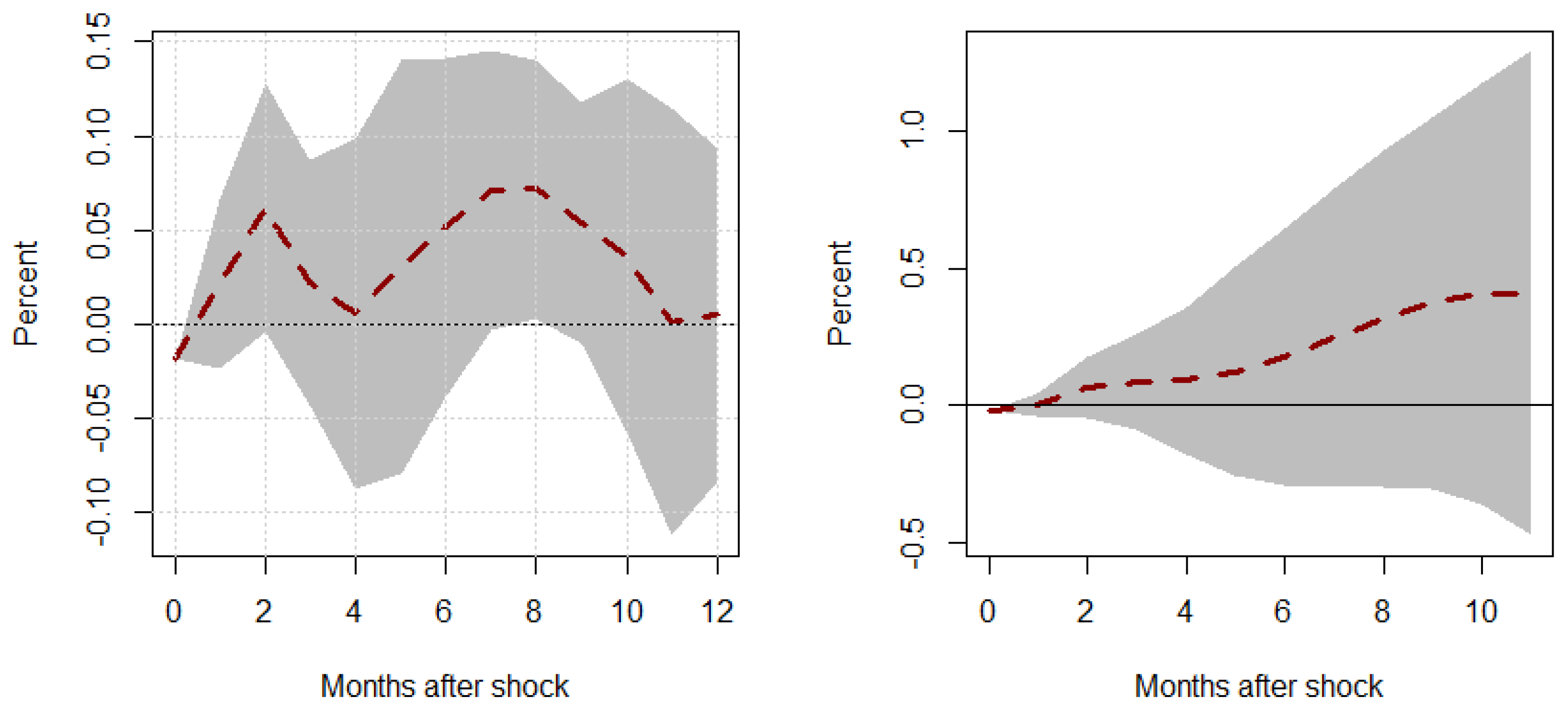
Figure 4.
Responses to a unit Shock–Regime 1. This figure shows the transitory (left panel) and cumulative (right panel) responses of global supply chain pressure, , to a unit oil price inflation shock, , under a regime where . The shaded region represents the 95% confidence intervals associated with our responses.
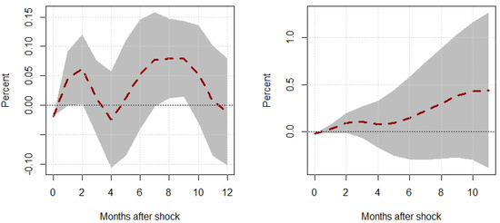
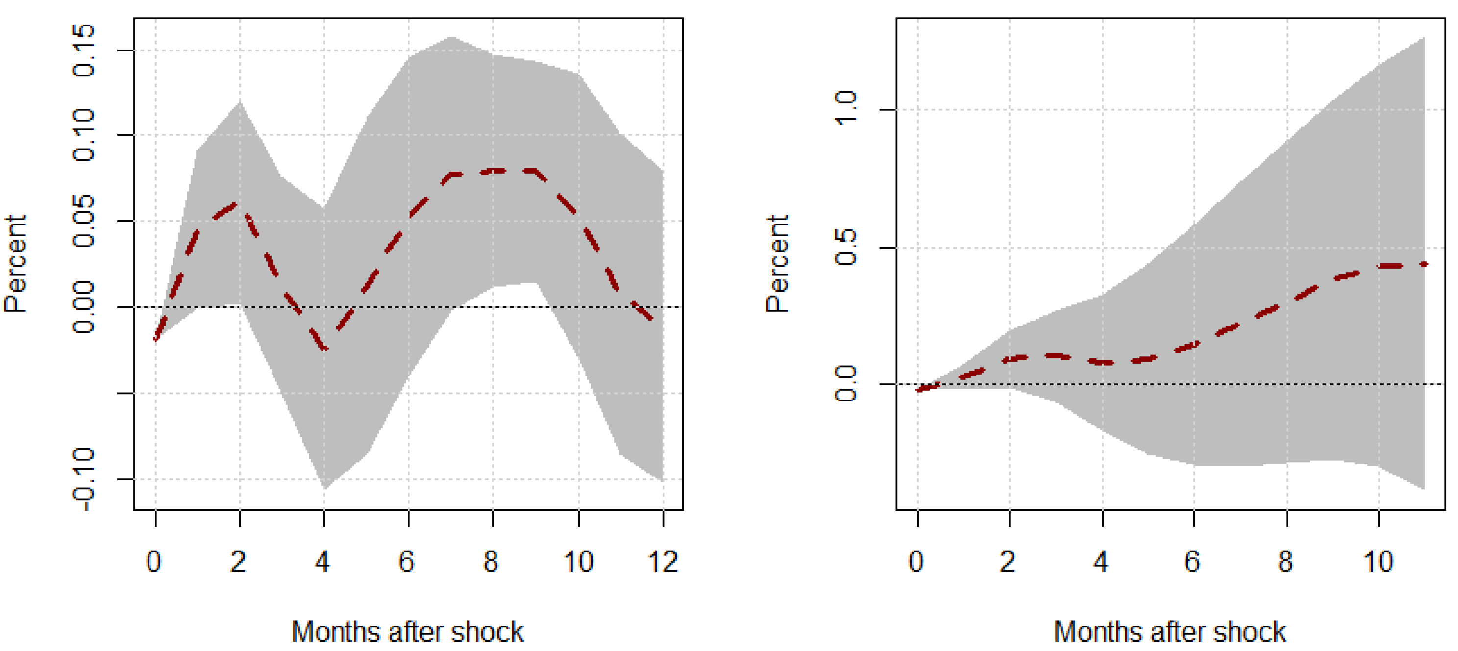
Figure 5.
Responses to a unit Shock–Regime 2. This figure shows the transitory (left panel) and cumulative (right panel) responses of global supply chain pressure, , to a unit oil price inflation shock, , under a regime where . The shaded region represents the 95% confidence intervals associated with our responses.
5. Discussion
Our results tell a very interesting story. As per Figure 4, the mean response of supply chain pressure after an oil price shock under periods of higher-than-trend political uncertainty is around 10%, peaking at around 14%. Furthermore, these shocks tend to have a permanent impact, as even after a 12-month forecast horizon, supply chain pressures usually do not revert back to the trend, suggesting that dynamic supply chain pressure is fairly rigid, much like consumer price inflation, persisting at higher levels of duress post-shock in both the transitory response and the cumulative response. On the other hand, the cumulative responses exhibit much wider confidence intervals yet still exhibit a peak mean response of around 100% after 12 months but can be as low as 25%, roughly speaking.
Looking at the second set of responses in Figure 5, we see that in periods of time where there are no statistically significant responses of supply chain pressure to oil price shocks. This finding is significant when contrasted with Figure 4. We observe that when political uncertainty or stability is relatively low, supply chain pressure is more resilient or insulated from shocks. On the other hand, when political uncertainty is relatively higher, we observe that oil price shocks can drive supply chain pressure upward by a non-trivial magnitude.
In terms of the relevancy of our findings, and as noted in Jiang et al. (2022), COVID-19 was an event that exposed the fragility of many integral global value chains. Jiang et al. (2022) argues that the previous focus on efficient supply chains, specifically just-in-time philosophies, is not sufficient for insulating supply chains from systemic and idiosyncratic shocks, thus the need for more resilient and robust supply chain frameworks is imperative for insulating macroeconomic welfare from a variety of supply chain distortions. In our setting, oil price shocks represent an event that can also shatter the stability of otherwise efficient, yet not robust, value chains. As per our motivating question, we asked ourselves if political uncertainty (or lack thereof) can exacerbate the instability of supply chains under events like oil price shocks. Our results illustrate that regardless of how robust supply chains may be at a macroeconomic level, lower levels of political uncertainty do not have a statistically significant impact on the responses of supply chain disruption to energy shocks, but periods of political instability or higher levels of uncertainty can greatly amplify the degree to which supply chain disruption is worsened under oil price shocks.
This is further reinforced in Fornaro and Wolf (2023), who point out the nature of energy shocks as an amplifier of supply chain disruption, which induces negative wealth effects and contractions in the business cycle that persist long after the shocks are elicited. Fornaro and Wolf (2023) refer to this effect as “scarring”. Our results, particularly Figure 4, echo these findings. Fornaro and Wolf (2023) also point out that policy actions and a mix of monetary and fiscal policy actions can serve to reign in or counteract the effects of energy or pandemic shocks on supply chain disruption, which is again affirmed by our results in Figure 5.
While more narrow in scope, there is an adjacent literature concerned with the supply chain resiliency of food and agricultural commodities. Works like Davis et al. (2021) stress the role of policymakers as mitigators of supply chain disruptions within the food and agricultural commodity value chains. Our results from Figure 4 and Figure 5 confirm this more generally in that the nature of political uncertainty may not “help” dampen shocks per se but can at the very least mitigate the severity of disruptions that would otherwise put upward pressure on the economy at large.
Potential Mechanisms
A natural discussion to be had herein is the potential mechanisms at play driving our results. By extension, we ask if some of the variation in supply chain volatility we observe under political uncertainty is explained by the precautionary behavior or investment delays on behalf of firms? To this end, we turn to the inventories literature and gather data on real total business inventories from the Bureau of Labor Statistics, , and use it as a variable of interest in a local projection impulse–response function, wherein we evaluate the impact of oil price shocks within our two-regime framework (we convert real inventories into inventory investment, for satisfying the stationarity conditions essential for our modeling framework). Figure 6 and Figure 7 show the transitory and cumulative responses of inventory investment behavior under regimes of higher-than-trend political uncertainty and at the trend-or-lower levels of political uncertainty.
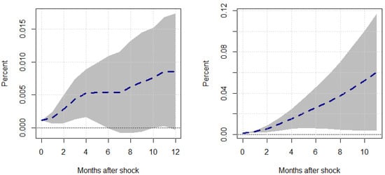
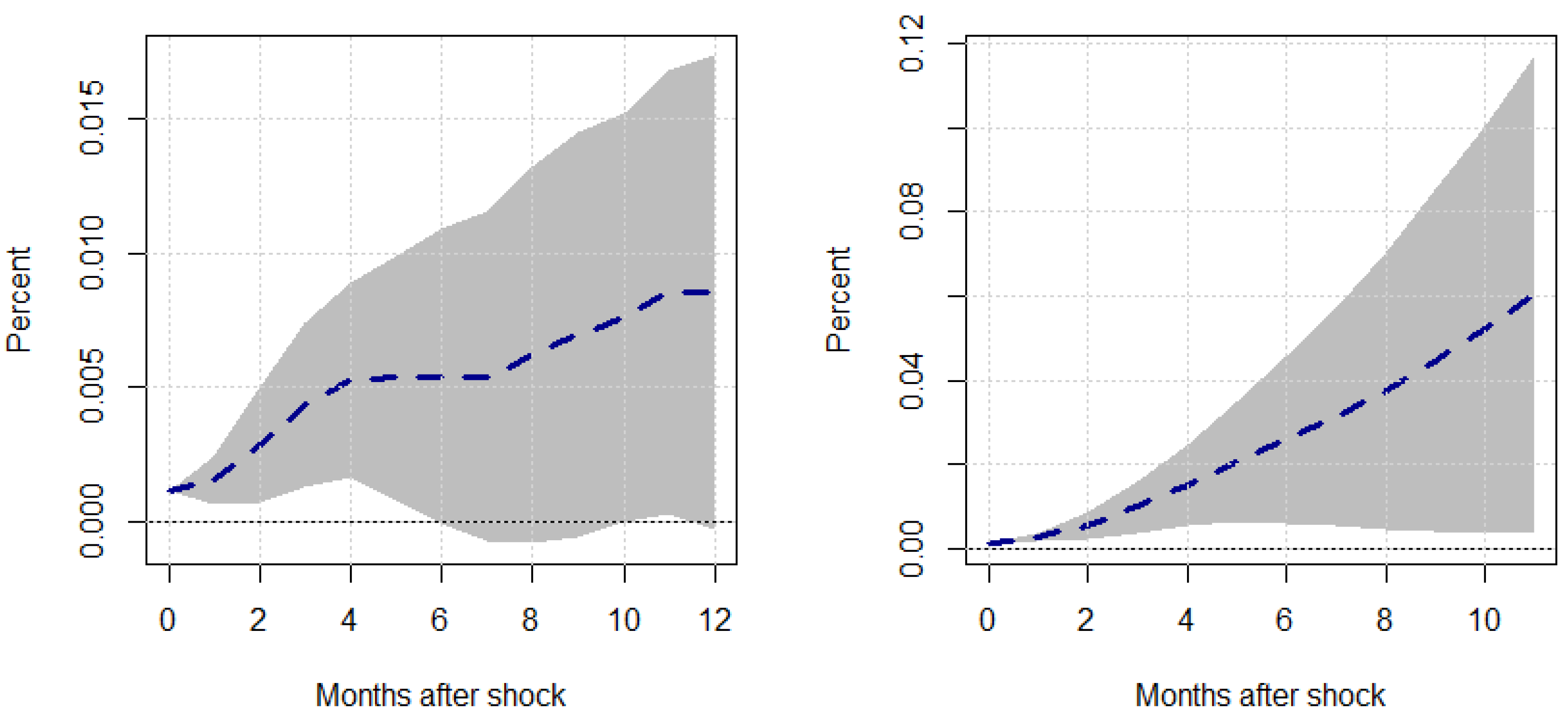
Figure 6.
Responses to a unit Shock–Regime 1. This figure shows the transitory (left panel) and cumulative (right panel) responses of inventory investment, , to a unit oil price inflation shock, , under a regime where . The shaded region represents the 95% confidence intervals associated with our responses.
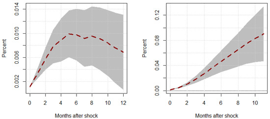
Figure 7.
Responses to a unit Shock–Regime 2. This figure shows the transitory (left panel) and cumulative (right panel) responses of inventory investment, , to a unit oil price inflation shock, , under a regime where . The shaded region represents the 95% confidence intervals associated with our responses.
Taken together, these results are quite telling. During periods of higher political uncertainty, inventory investment tends to be relatively weaker statistically and very volatile (wider confidence intervals). In comparison, when political uncertainty is low or at expected levels, inventory investment tends to be much stronger statistically speaking, and far less volatile. This is consistent with the literature on the recent advances at the intersection of inventories and energy shocks.
For example, Herrera (2018) points out that oil prices have a tendency to deter inventory investment in oil-intensive energies, thereby suggesting a delay in investment due to heightened industry costs. On the other hand, Alquist et al. (2020) would point out that oil price shocks can deter investment demand via a depreciation of the U.S. dollar, again suggesting that investment delays tend to explain the mechanisms underlying most firm-level inventory investment reactions to energy shocks. Figure 6 largely affirms these findings; however, Figure 7 suggests that when political uncertainty is minimal, firms actually increase their inventories, while under a positive oil price shock, it is perhaps out of caution. While these tertiary results warrant a separate study on their own, it seems evident that higher levels of political uncertainty coincide with investment delays, while lower levels of uncertainty create incentives for precautionary firm investment.
6. Extensions
We consider two extensions of our initial frame: a replication of our initial results with news uncertainty as our switching variable for our local projection models to test for the robustness of our results to alternative measures of risk and uncertainty; and a two-step time-varying VAR framework to capture “smoother” effects or nonlinearities in the influence that uncertainty has over oil prices, as manifested in direct oil price shocks to supply chain pressure. One could argue that this is an alternative, albeit slightly less efficient, approach to capturing our initial results.
6.1. News Cycle
A natural extension of our main results is to consider alternative indices of broader socioeconomic or sociopolitical uncertainty. Of growing interest to researchers is the role that “news shocks” play in the broader business cycle with works such as Barsky and Sims (2011) and Berger et al. (2020). Fundamentally, news shocks broadly capture changes in expectations about the future, particularly concerning technological progress or productivity, that affect current economic activity, even though the actual changes may occur later.
These shocks are considered to be unexpected information that influences economic decisions and outcomes. These shocks are forward-looking in nature and offer an alternative to political uncertainty from which to extend our initial results. A news uncertainty measure is available from the same principle source as our political uncertainty index. To reproduce our econometric analysis and simulations, we first extract the cyclical component of our news uncertainty measurement in the same manner as we extracted our policy uncertainty cycle measure. Our news cycle measure compared to our initial index and our trend component is described in Figure 8. A comparison between our cyclical measure of policy uncertainty and our news uncertainty alternative is described in Figure 9
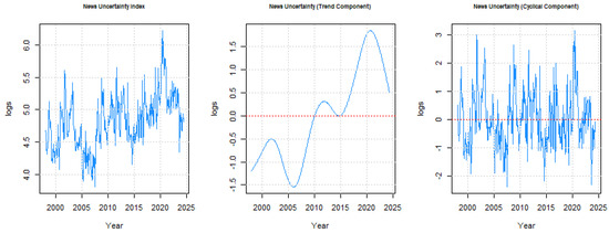
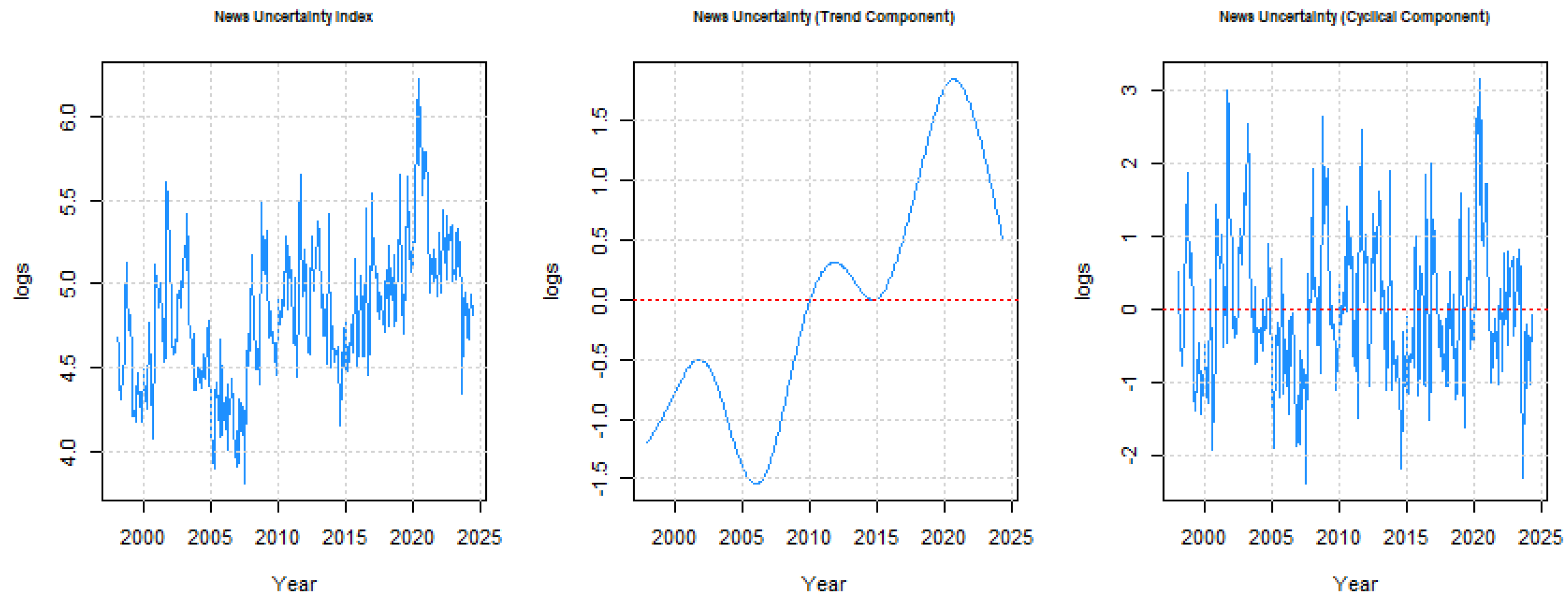
Figure 8.
News uncertainty index decomposition. This figure shows our news uncertainty index, (left panel), the demeaned trend component, (middle), and our demeaned cyclical component, (right panel).
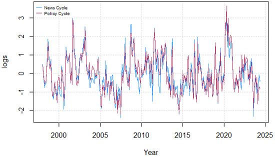
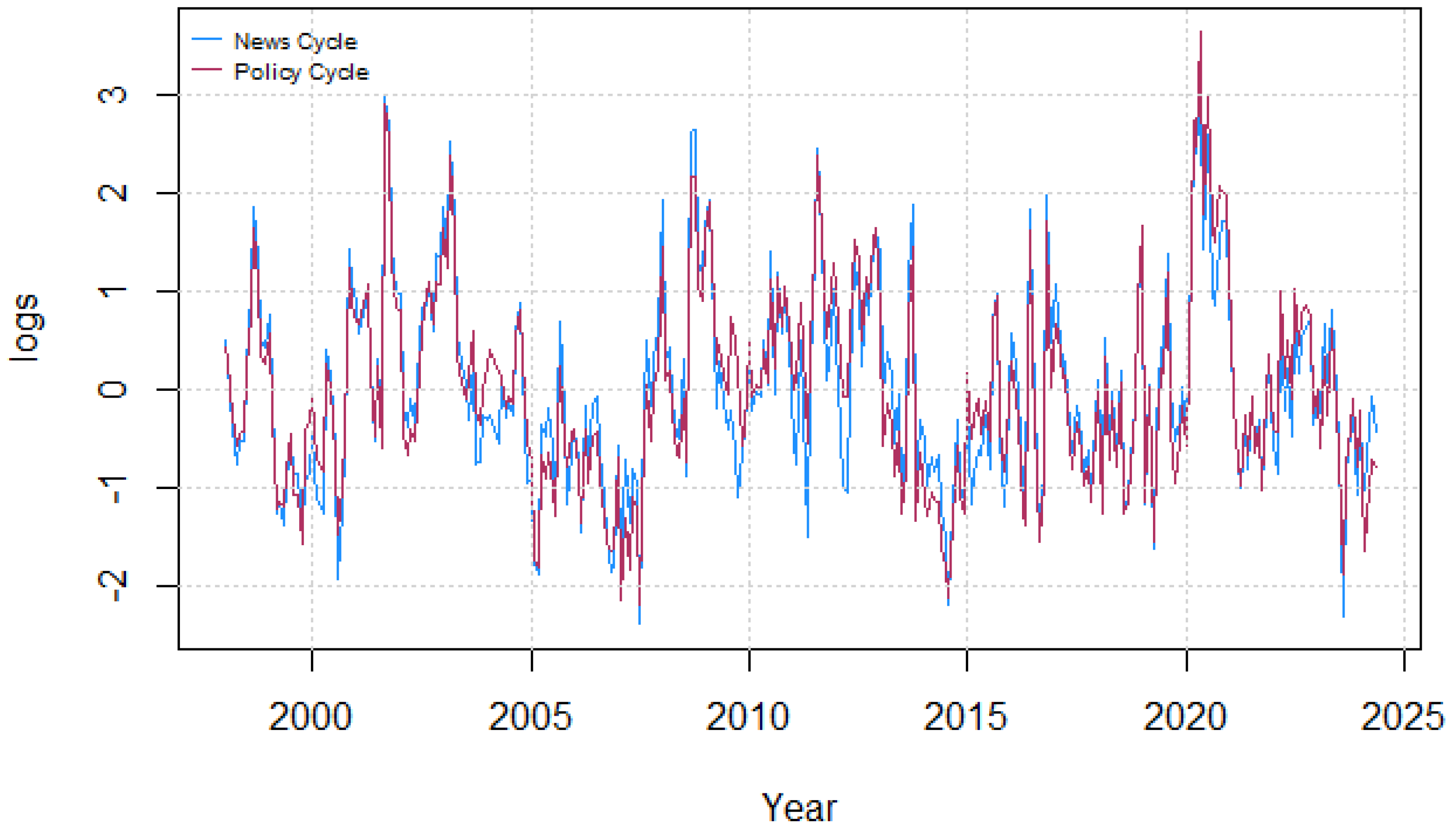
Figure 9.
Comparison of news uncertainty to political uncertainty. This figure compares our two measures of cyclical uncertainty.
With this in mind, we can fit a series of cumulative and noncumulative local projection impulse–response functions similar in specification to our main results, but with our switching variable being the news cycle, , rather than the policy cycle. Figure 10 and Figure 11 illustrate these respective responses.
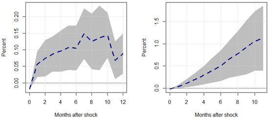
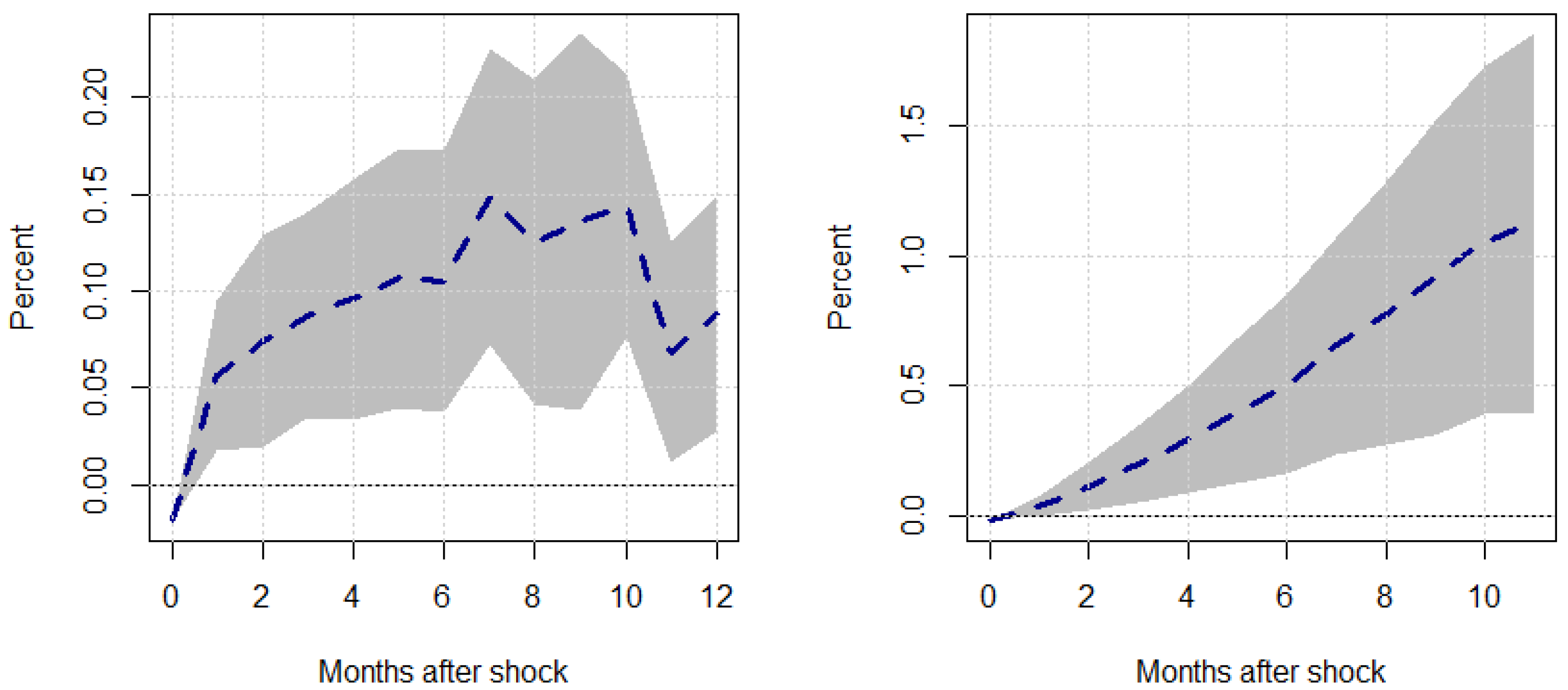
Figure 10.
Responses to a unit Shock–Regime 1. This figure shows the transitory (left panel) and cumulative (right panel) responses of global supply chain pressure, , to a unit oil price inflation shock, , under a regime where . The shaded region represents the 95% confidence intervals associated with our responses.

Figure 11.
Responses to a unit Shock–Regime 2. This figure shows the transitory (left panel) and cumulative (right panel) responses of global supply chain pressure, , to a unit oil price inflation shock, , under a regime where . The shaded region represents the 95% confidence intervals associated with our responses.
As we can see, there is minimal economic or statistical difference between a measure of uncertainty associated with news-based cycles or policy-based cycles, affirming our initial results and interpretation.
6.2. Time-Varying Responses
Related to recent contributions in the space of oil shocks, many researchers have started to evaluate the relationship between oil shocks and key macroeconomic indicators within a time-varying framework. Works like Baumeister and Peersman (2013) and Cross and Nguyen (2017), among others, utilize methods like time-varying vector autoregressive (TVVAR) analysis to quantify the responsive of key indicators to oil price shocks, while accounting for time-dependent nonlinearities.
To this end, we explore the potential of a time-varying framework, the potential to smoothly incorporate political uncertainty into supply chain pressure responses to energy shocks. To achieve this, we employ a two-step framework: first, we regress oil price inflation on the cyclical component of our policy uncertainty measure, and save the residual vector; secondly, we construct a bivariate time-varying VAR, where our vector of endogenous variables consists of supply chain pressure, and our residual “shock” variable from our first-stage model. Formally, the first-stage equation that identifies our shock is described by Equation (12).
Equation (12) allows us to obtain , which is incorporated alongside into a bivariate vector of endogenous variables that will be utilized for estimating a time-varying VAR described by Equation (13), with lags as per the AIC criteria.
where the parameters , , and are smooth functions of t, time. When constructing impulse–response functions, we will have values of each response variable projected over h forecast periods; therefore, each impulse response function for a single variable’s response to a single shock will have observations. To present our impulse–response functions graphically, we take the average of all smooth estimates across each forecast period. This produces an average response that supplements our initial results. Specifically, we are interested in the response of to a shock. Figure 12 illustrates this response.
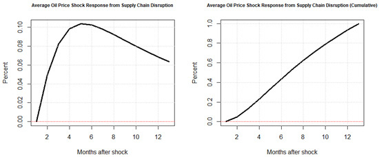
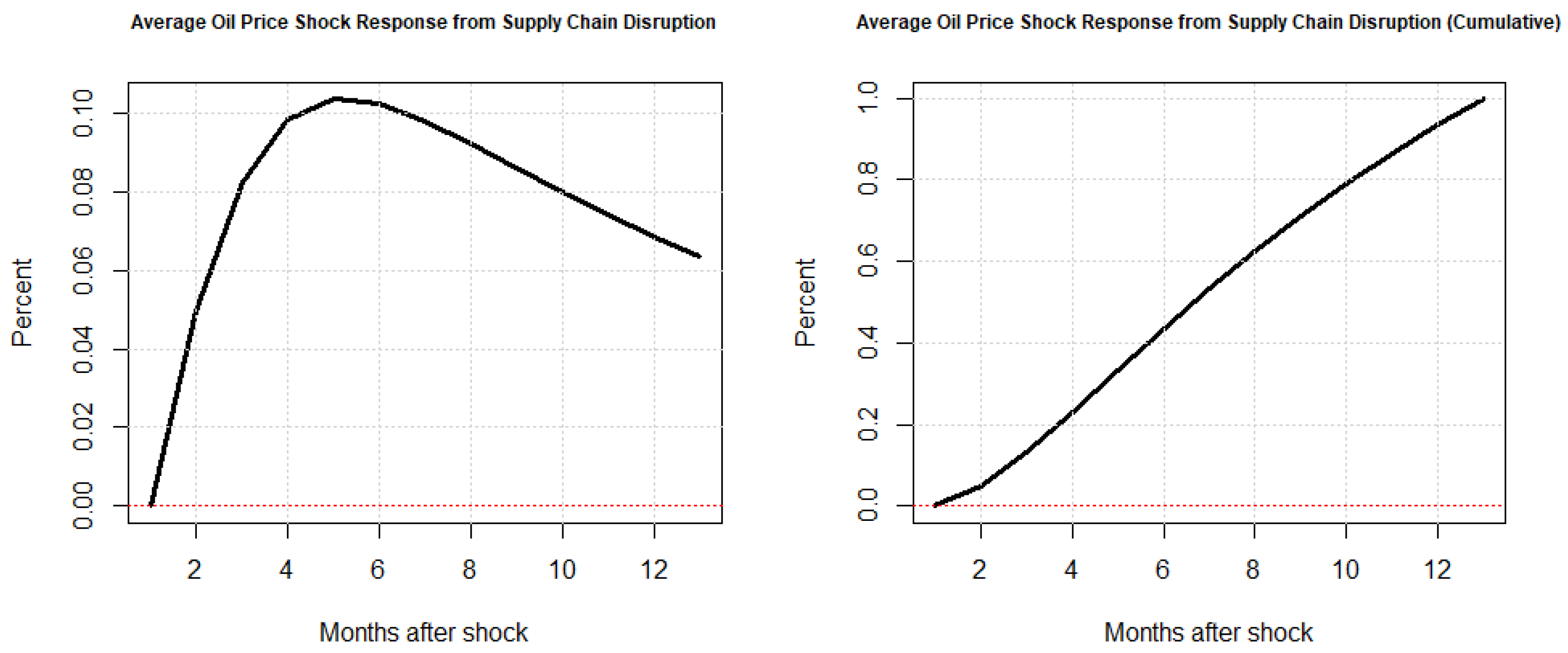
Figure 12.
Average response of supply chain pressure to oil price innovations. This figure represents the mean of the time-varying impulse–response function over every time period with shocks projected months ahead.
Our time-varying results are in the same vein as our initial simple VAR with transitory responses of supply chain pressures to oil price shocks resulting in a roughly ten percent increase in general supply chain stress after around the five-month mark with a slow reversion back to the zero line. Cumulatively, we see after a 12-month period that such an innovation from energy markets roughly doubled global supply chain duress.
7. Concluding Remarks
In summary, our analysis highlights the intricate relationship between political uncertainty and supply chain pressures in the context of oil price shocks and their subsequent effects on supply chain pressure. Our findings, as illustrated in Figure 4 and Figure 5, reveal that periods of heightened political uncertainty significantly amplify the impact of oil price shocks on supply chain pressures, leading to both immediate and persistent disruptions. Specifically, during high uncertainty periods, supply chain pressures can rise notably, peaking at substantial levels and remaining elevated over time. Conversely, when political stability is high, the response of supply chains to oil price shocks is statistically insignificant, suggesting a more resilient system is achievable under stable political conditions.
These insights are consistent with recent literature emphasizing the fragility of global supply chains exposed by shocks such as those induced by the COVID-19 pandemic and energy crises. The evidence supports the argument that while efficient supply chains are crucial, they are insufficient in isolation for mitigating systemic disruptions. Instead, incorporating robust frameworks that can withstand both systemic and idiosyncratic shocks is essential for maintaining macroeconomic stability.
Our findings resonate with the concept of “scarring” described by Fornaro and Wolf (2023), where energy shocks exacerbate long-term supply chain disruptions and induce pervasive, negative welfare outcomes like higher inflation and lower household wealth. Moreover, our results align with Jiang et al. (2022), which underscores the need for resilience beyond mere efficiency. The role of policymakers, as highlighted in adjacent literature, becomes crucial in mitigating these effects, suggesting that while political uncertainty cannot entirely dampen the severity of supply chain shocks, it can influence the magnitude of disruption and inform strategic policy responses.
Finally, we acknowledge that our study is not without limitations, and warrants further extensions. Firstly, we use data available strictly for the United States and only over a relatively recent sample period due to data limitations with the supply chain pressure index; therefore, future research would do well to not only extend our study and its scope to other nations or regions outside the United States but also explore different measures of supply chain pressure. Beyond these surface-level limitations, we take a very broad look at the relationship between political uncertainty, and supply chain pressure through oil price shocks; however, political uncertainty is often tied to election cycles and election expectations, which may carry more variation at a higher level of granularity than the data we utilize. Thus future studies could recontextualize our research within election cycles specifically, rather than political uncertainty more abstractly.
Overall, our results underline the importance of integrating political stability considerations into supply chain management and policy formulation, especially in the face of energy price shocks, to better manage and mitigate the associated economic impacts. We stress that our main methodological contribution is analyzing the intersection of the three distinct literature fields of supply chain pressure, political uncertainty, and oil price shocks in a single unifying framework, rather than separately from one another. Moreover, our results suggest that concerted efforts or mechanisms that reduce policy uncertainty can mitigate the pass-through of oil demand shocks to supply chain pressures, which has indirect implications for dampening inflation pangs stemming from either supply chain volatility (upward pressure on prices permeating through the value chain) or oil price pass-through.
Funding
This research received no external funding.
Institutional Review Board Statement
Not applicable.
Informed Consent Statement
Not applicable.
Data Availability Statement
The original contributions presented in this study are included in the article.
Conflicts of Interest
The authors declare no conflicts of interest.
Notes
| 1 | Formally, we use the West Texas Instruments (WTI) data series of crude oil prices for the United States. |
| 2 | Following Jordà (2005), is obtained from a state-independent structural VAR (SVAR) following a form similar to Equation (9). This is done automatically using the “lpirfs” package in the statistical software, R. See Adämmer (2019) for details and documentation. |
References
- Acemoglu, D., & Tahbaz-Salehi, A. (2024). The macroeconomics of supply chain disruptions. Review of Economic Studies, 92, 656–695. [Google Scholar] [CrossRef]
- Adämmer, P. (2019). lpirfs: An R package to estimate impulse response functions by local projections. The R Journal, 11(2), 421–438. [Google Scholar] [CrossRef]
- Alquist, R., Ellwanger, R., & Jin, J. (2020). The effect of oil price shocks on asset markets: Evidence from oil inventory news. Journal of Futures Markets, 40(8), 1212–1230. [Google Scholar] [CrossRef]
- Balcilar, M., Bekiros, S., & Gupta, R. (2017). The role of news-based uncertainty indices in predicting oil markets: A hybrid nonparametric quantile causality method. Empirical Economics, 53, 879–889. [Google Scholar] [CrossRef]
- Baldwin, R., & Freeman, R. (2022). Risks and global supply chains: What we know and what we need to know. Annual Review of Economics, 14(1), 153–180. [Google Scholar] [CrossRef]
- Barsky, R. B., & Kilian, L. (2002). Oil and the macroeconomy since the 1970s. Journal of Economic Perspectives, 18(4), 115–134. [Google Scholar] [CrossRef]
- Barsky, R. B., & Sims, E. R. (2011). News shocks and business cycles. Journal of monetary Economics, 58(3), 273–289. [Google Scholar] [CrossRef]
- Baumeister, C., & Peersman, G. (2013). Time-varying effects of oil supply shocks on the US economy. American Economic Journal: Macroeconomics, 5(4), 1–28. [Google Scholar] [CrossRef]
- Bekiros, S., Gupta, R., & Paccagnini, A. (2015). Oil price forecastability and economic uncertainty. Economics Letters, 132, 125–128. [Google Scholar] [CrossRef]
- Berger, D., Dew-Becker, I., & Giglio, S. (2020). Uncertainty shocks as second-moment news shocks. The Review of Economic Studies, 87(1), 40–76. [Google Scholar] [CrossRef]
- Blanchard, O. J., & Gali, J. (2007). The macroeconomic effects of oil shocks: Why are the 2000s so different from the 1970s? National Bureau of Economic Research Cambridge. [Google Scholar]
- Cross, J., & Nguyen, B. H. (2017). The relationship between global oil price shocks and China’s output: A time-varying analysis. Energy Economics, 62, 79–91. [Google Scholar] [CrossRef]
- Davis, K. F., Downs, S., & Gephart, J. A. (2021). Towards food supply chain resilience to environmental shocks. Nature Food, 2(1), 54–65. [Google Scholar] [CrossRef] [PubMed]
- Diaz, E. M., Cunado, J., & de Gracia, F. P. (2023). Commodity price shocks, supply chain disruptions and US inflation. Finance Research Letters, 58, 104495. [Google Scholar] [CrossRef]
- Engemann, K. M., Kliesen, K. L., & Owyang, M. T. (2011). Do oil shocks drive business cycles? Some US and international evidence. Macroeconomic Dynamics, 15(S3), 498–517. [Google Scholar] [CrossRef]
- Fernández-Villaverde, J., & Guerrón-Quintana, P. A. (2020). Uncertainty shocks and business cycle research. Review of Economic Dynamics, 37, S118–S146. [Google Scholar] [CrossRef]
- Fornaro, L., & Wolf, M. (2023). The scars of supply shocks: Implications for monetary policy. Journal of Monetary Economics, 140, S18–S36. [Google Scholar] [CrossRef]
- Gundersen, T. S. (2020). The impact of US supply shocks on the global oil price. The Energy Journal, 41(1), 151–174. [Google Scholar] [CrossRef]
- Herrera, A. M. (2018). Oil price shocks, inventories, and macroeconomic dynamics. Macroeconomic Dynamics, 22(3), 620–639. [Google Scholar] [CrossRef]
- Herrera, A. M., Karaki, M. B., & Rangaraju, S. K. (2019). Oil price shocks and US economic activity. Energy Policy, 129, 89–99. [Google Scholar] [CrossRef]
- Hodrick, R. J., & Prescott, E. C. (1997). Postwar US business cycles: An empirical investigation. Journal of Money, Credit, and Banking, 1, 1–16. [Google Scholar] [CrossRef]
- Jiang, B., Rigobon, D., & Rigobon, R. (2022). From Just-in-Time, to Just-in-Case, to Just-in-Worst-Case: Simple Models of a Global Supply Chain under Uncertain Aggregate Shocks. IMF Economic Review, 70(1), 141–184. [Google Scholar] [CrossRef]
- Jiménez-Rodríguez, R. (2022). Oil shocks and global economy. Energy Economics, 115, 106373. [Google Scholar] [CrossRef]
- Jordà, Ò. (2005). Estimation and inference of impulse responses by local projections. American Economic Review, 95(1), 161–182. [Google Scholar] [CrossRef]
- Kang, W., Ratti, R. A., & Vespignani, J. L. (2017). Oil price shocks and policy uncertainty: New evidence on the effects of US and non-US oil production. Energy Economics, 66, 536–546. [Google Scholar] [CrossRef]
- Kilian, L., Rebucci, A., & Spatafora, N. (2009). Oil shocks and external balances. Journal of International Economics, 77(2), 181–194. [Google Scholar] [CrossRef]
- Nitsche, B., & Durach, C. F. (2018). Much discussed, little conceptualized: Supply chain volatility. International Journal of Physical Distribution & Logistics Management, 48(8), 866–886. [Google Scholar]
- Nordhaus, W. D. (2007). Who’s afraid of a big bad oil shock? Brookings Papers on Economic Activity, 2007(2), 219–238. [Google Scholar] [CrossRef]
- Odulaja, B. A., Oke, T. T., Eleogu, T., Abdul, A. A., & Daraojimba, H. O. (2023). Resilience in the face of uncertainty: A review on the impact of supply chain volatility amid ongoing geopolitical disruptions. International Journal of Applied Research in Social Sciences, 5(10), 463–486. [Google Scholar] [CrossRef]
- Ravn, M. O., & Uhlig, H. (2002). On adjusting the Hodrick-Prescott filter for the frequency of observations. Review of Economics and Statistics, 84(2), 371–376. [Google Scholar] [CrossRef]

Disclaimer/Publisher’s Note: The statements, opinions and data contained in all publications are solely those of the individual author(s) and contributor(s) and not of MDPI and/or the editor(s). MDPI and/or the editor(s) disclaim responsibility for any injury to people or property resulting from any ideas, methods, instructions or products referred to in the content. |
© 2025 by the author. Licensee MDPI, Basel, Switzerland. This article is an open access article distributed under the terms and conditions of the Creative Commons Attribution (CC BY) license (https://creativecommons.org/licenses/by/4.0/).