The Economy-Wide Impact of Harnessing Human Capital Development and the Case of Ethiopia: A Dynamic Computable General Equilibrium Model Analysis

Abstract

This study uses a computable general equilibrium (CGE) model to analyze the impact of skilled and semi-skilled labor supply shocks on the Ethiopian economy and sectoral outputs. The study examines three policy scenarios: a 10% increase, a 15% increase, and a 20% increase in skilled and semi-skilled labor supply compared to a business-as-usual (BAU) scenario. The findings show that all three scenarios contribute to higher economic growth, investment, and exports. The impact on sectoral outputs is also significant, with the industry and services sectors performing better than the agriculture sector. In the 20% increase scenario, the real annual gross domestic product (GDP) growth rate is projected to be 0.79 percentage points higher than the business-as-usual scenario. Additionally, the annual growth rates of investments and exports are expected to be 2.69 and 2.31 percentage points higher, respectively, compared to their business-as-usual scenario counterparts. The agriculture sector experiences a slight increase of 0.16 percentage points in annual production compared to the business-as-usual scenario. Output in the industry sector also sees a rise of 1.61 percentage points higher than the business-as-usual scenario, while outputs in the services sector improve significantly. Overall, the study highlights the positive impact of increasing the supply of skilled and semi-skilled labor on the economy. This is mainly due to the higher productivity of skilled and semi-skilled workers, which contributes to increased economic growth. The findings suggest that governments should implement policies to enhance the supply of skilled and semi-skilled labor, such as investing in education and training programs. These measures would promote economic growth and improve living standards.

1. Introduction

1.1. Background of the Study

Since the 1980s, the crucial role of human capital in driving economic growth and reducing poverty has been widely recognized. Over the years, various theories that explore the impact of human capital on economic growth and development have emerged. These theories underscore that human capital comprising the skills, talents, education, and abilities of the workforce plays a fundamental role in the development process. From a macroeconomic perspective, the accumulation of human capital enhances labor productivity, fosters technological innovation, increases returns on capital, and promotes sustainable growth. Human capital development is crucial for achieving sustainable development goals, as it enhances productivity, innovation, and economic growth (see Klarin, 2018; Manioudis & Meramveliotakis, 2022). Consequently, it is a key element in the economy-wide production function and contributes significantly to poverty reduction.

At the microeconomic level, education, which serves as a proxy for human capital, enhances individual employability in the labor market and increases earning potential. Thus, at an individual level, human capital directly influences labor productivity and earnings, making it an integral component of firm production. In this context, human capital refers to an individual’s ability and efficiency in transforming raw materials and capital into goods and services. There is a consensus that these skills can be developed through the educational system.

In growth theory, Solow-Swan’s growth model is considered the main model of growth theory. Alternative economic growth models are often compared to it. The Solow-Swan growth model, also known as the neoclassical growth model, concludes that long-term economic growth cannot be achieved by simply accumulating capital without technological progress. This is because of the assumption of diminishing returns, which eventually limits growth (Savvides & Stengos, 2009; Acemoglu et al., 2019; D. Romer, 2019). Technological improvements are necessary to overcome the effects of diminishing returns, as they make factors, such as labor, more productive. In the human capital extended neoclassical growth model proposed by Mankiw et al. (1992), both physical and human capital are included in the production function. It was found that technological progress is still the main source of growth (Savvides & Stengos, 2009).

An alternative growth model to counter the impact of diminishing returns is to consider a production function that does not adhere to the principle of diminishing returns. This model, known as the AK model, assumes that the output is a linear function of capital. Consequently, economies characterized by this type of production function can continuously accumulate physical capital without experiencing diminishing returns. The AK model appears to be a modified version of the Harrod-Domar growth model, which posits that the rate of output growth is determined by the ratio of savings and capital-output ratios. The proposition of this growth model is that, given the low savings rate and high capital-output ratio resulting from capital scarcity in many developing countries, it is crucial to accelerate growth by increasing the savings rate. This will enable the absorption of the growing labor force and reduce poverty (Ararat, 2009).

However, in the endogenous growth model, the process of technical change or knowledge accumulation is not constant or predetermined; it depends on the specific features of the model. Knowledge accumulation can be understood as the adoption of new production techniques, the implementation of new management and organizational structures, and the accumulation of scientific knowledge. Such knowledge accumulation can enhance the level of human capital in the economy, which in turn has a positive effect on economy’s productive capacity (Savvides & Stengos, 2009). Therefore, the accumulation of human capital is useful in overcoming the limitations of diminishing returns and can lead to economic growth, even in the absence of technological progress, at least in the short term. It is widely acknowledged that sustainable long-term growth can be achieved through continuous improvement of the production process through the adoption of new technologies and methods. In this context, P. M. Romer (1990) argues that the development of human capital leads to higher economic growth, as educated workers contribute to innovation through research and development activities (P. M. Romer, 1990). Thus, human capital plays a crucial role in increasing productivity rates by facilitating the faster rate of innovation in domestic products and services, as well as by imitating technologies developed elsewhere.

1.2. Human Capital Development in Ethiopia

Ethiopia, home to a population of over 120 million in 2021, is the second most populous country in Africa. The country has a youthful population, with 40% of Ethiopians under the age of 15. However, the agricultural sector, which is facing a decline in available land per farmer, may struggle to provide employment opportunities for this growing youth bulge. Schmidt and Woldeyes (2019) have shed light on this issue, indicating that without proactive management, these young individuals may face unemployment, leading to untapped potential and discontent. However, with the right policies in place, Ethiopia’s youthful population could become an asset in driving the country’s development agenda, which is aimed at poverty reduction.

From an individual standpoint, research suggests that individuals with higher levels of education tend to have better employment prospects, higher earnings, and greater productivity compared to those with lower levels of education. These findings have provided a strong rationale for governments and households to invest a significant proportion of their resources in education. The hope is that these investments will yield long-term benefits for both the economy and households. Education is seen as an investment that equips individuals with the knowledge and skills necessary for improved employment opportunities and enhanced productive capacities.

Recognizing that education plays a critical role in preparing the youth for the transition from an agrarian to a modern society, the Government of Ethiopia has allocated substantial funds to the education sector in recent years. As a result, the number of formal education centers has increased, leading to a significant rise in youth enrollment. Since 2015/16, school enrollment has exceeded 20 million and 2.4 million students in primary and secondary schools, respectively as shown in

Table 1. Formal education developments.

Particulars	2014/15	2015/16	2016/17	2017/18	2018/19	2019/20	2020/21
Primary schools	33,373	34,867	35,887	36,437	37,039	37,742	35,980
Secondary schools	2830	3156	3380	3589	3739	3687	3481
No. of universities	33	37	37	49	50	55	56
School enrolment
Primary (million)	18.7	20	20.8	20.7	20.04	20.4	18.4
Secondary (million)	2.11	2.42	2.56	2.67	2.82	3.47	3.54
TVET (thousands)	265.75	304.14	302.08	292.38	317.73	386.81	283.97

Source: (National Bank of Ethiopia, 2021).

. The number of primary and secondary schools has reached 37,742 and 3687, respectively, in the 2019/20 academic year. The student population in primary and secondary schools has surpassed 20.4 million and 3.4 million, respectively, in 2019. Additionally, the number of technical and vocational education and training (TVET) centers has also seen growth.

Despite the commendable increase in the number of students, there are concerns regarding the quality of education, as a large portion of primary school students do not progress to secondary education. Furthermore, there exist regional disparities in terms of access to education. The fact that students fail to complete secondary education decreases their likelihood of benefiting from employment opportunities.

Ethiopia has also prioritized technical and vocational education and training (TVET) as part of its education strategy. The TVET centers aim to develop the skills of the youth and help them enter the labor market. As of 2015/16, there were over 300,000 students in TVET institutions. However, Krishnan and Shaorshadez (2013) argue that the TVET program in Ethiopia has been supply-driven, despite the strategy emphasizing flexibility in accommodating the demand for TVET students (Krishnan & Shaorshadez, 2013).

Investing in education is a crucial policy tool available to policymakers. The Incheon Declaration for implementing Sustainable Development Goal 4 recommends allocating 4% to 6% of the GDP or 15% to 20% of total government expenditure to education (UNESCO, 2015). In Ethiopia, as illustrated in Figure 1, the share of education expenditure as a proportion of total government expenditure has increased, reaching 24% in 2018 compared to 14% in 1994. In fact, Ethiopia has surpassed the internationally set target of 20% total expenditure on education.

As illustrated in Figure 2, Ethiopia has consistently allocated more than 4% of its GDP to education since 2005. This indicates a substantial commitment to advancing education within the country. Consequently, there has been notable progress in expanding access to education. Nevertheless, there is anecdotal evidence suggesting that the anticipated impact on development has not been fully realized. According to Pritchett (2001), this lackluster performance in various developing nations can be attributed to factors such as unfavorable governance conditions, diminishing marginal returns, and inadequate education quality (Pritchett, 2001).

As of 2018, the total education expenditure amounted to USD 3.4 billion (or ETB 92.6 billion), showing significant growth from just USD 1 billion a decade ago. Over the past few decades, education expenditure has increased both in terms of share and absolute levels, as well as per capita.

Despite the substantial public investment in education, the share of national income/gross national income (34%) in 2016 still went to laborers without formal education, although there was a slight decrease compared to 2011. Progress in this area has been slower than anticipated, considering the amount invested in the education sector.

The educational strategy has been carefully designed, with special attention given to technical and vocational education and training (TVET) as well as science and technology education. Furthermore, it is expected that the human capital development strategy will prioritize the linkage between universities (and TVET institutions) and industries. It is widely acknowledged that in-service training plays a crucial role in enhancing human capital development, as workers are more likely to specialize and acquire skills with moderate levels of training.

Table 2. The share of factors in value added in 2011.

Factors of Production	Share of Income
Lab—No Education	36.47
Lab—Primary Education	7.09
Lab—Secondary Education	7.37
Lab—Tertiary Education	5.70
Capital Land Rural	11.88
Capital Livestock Rural	4.07
Non-Agricultural Capital	26.45

Source: IFPRI SAM for 2011 (IFPRI, 2011).

and

Table 3. The share of factors in value added in 2016.

Factors of Production	Share of Income
Lab—No Education	34.05
Lab—Primary Education	7.37
Lab—Secondary Education	3.29
Lab—Tertiary Education	8.46
Capital Land Rural	7.32
Capital Livestock Rural	2.75
Non-Agricultural Capital	36.76

Source: PSI-EU SAM (PSI-EU, 2016).

illustrate an interesting trend: a shift in the utilization of human capital within the economy. The proportion of unskilled labor (Lab—No Education) has declined from 36.47% in 2011 to 34.04% in 2015/16, while the share of skilled labor (Lab—Tertiary Education) has increased from 5.70% in 2011 to 8.46% in 2015/16. This is accompanied by a rise in the contribution of non-agricultural capital, which has grown from 26.45% in 2011 to 36.76% in 2015/16. These figures indicate a structural transformation, suggesting that the economy is shifting its focus towards sectors with higher productivity, such as industry and services, and away from agriculture.

Given the government’s substantial investment in the education sector, which facilitates access to formal education and in-service training for a large proportion of the youth population, it is crucial to evaluate the contribution of skilled and semi-skilled workers to Ethiopia’s economic growth.

1.3. Objective

The objective of this study is to analyze the economy-wide impact of skilled biased technological progress on economic growth and income distribution.

The specific objectives are the following:

(i)

Analyze the effect of human capital development on economic growth and on sectoral output growth.

(ii)

Analyze the effects of skilled and semi-skilled labor supply shock on economic growth and other macroeconomic performances.

(iii)

Analyze the contribution of skilled and semi-skilled labor supply shock on sectoral growth and structural transformation.

(iv)

Investigate the effect of skilled biased labor supply shocks on factor income, government revenue and income changes by types of households.

This study is organized as follows. Section 2 provides a brief review of the literature on the relationship between human capital and economic growth. Section 3 describes the database and methodology used in the study. Section 4 presents the empirical results and discusses the main findings. Finally, Section 5 concludes the study and offers recommendations based on the findings.

2. Literature Review

The theory of economic growth has undergone significant development throughout various historical periods, resulting in the emergence of different perspectives. Modern growth theory, which traces its origins back to the influential work of Frank Ramsey in 1928, posits that prioritizing savings over current consumption yields higher levels of future consumption and output. However, in the aftermath of World War II, growth economists began formulating models based on the economies of developed nations, placing emphasis on factors like capital accumulation, technological advancements, and human capital as catalysts for economic growth.

The Harrod-Domar model, which is widely regarded as the first growth model in modern growth theories, emerged in the aftermath of the Great Depression. It provided a historical perspective and analyzed economic growth. The model synthesized the findings of studies conducted by Roy Harrod and Evsey Domar and explained an economy’s growth rate in terms of savings and capital (Harrod, 1939; Domar, 1946). Essentially, the model is a Keynesian model of economic growth that links an economy’s growth rate to the level of savings and capital. According to the Harrod-Domar growth model, the maximum rate of capital stock growth is determined by the ratio of the savings rate to the capital output ratio, assuming a historically determined and constant savings rate and capital output ratio (Ararat, 2009). If we assume that the rate of capital stock growth is the same as the rate of economic growth, and that the capital-output ratio is constant, then the economic growth rate becomes an increasing function of the savings rate.

The implication of the Harrod-Domar model is that, due to a low savings ratio but a high capital output ratio in developing countries, there will be a low growth a priori that cannot absorb the rapidly growing population. To address this, countries must accelerate economic growth beyond the traditional limits of the savings rate and capital output ratio by increasing the savings rate to a level that generates sufficient rates of economic growth to absorb the new labor force. The model assumes a direct relationship between output and capital stock, emphasizing the importance of physical capital accumulation (Savvides & Stengos, 2009). However, the Harrod-Domar model and other earlier models neglected the role played by technological advance and human capital in economic growth in their analyses.

On the other hand, the Solow-Swan neoclassical growth model is widely regarded as a foundational growth theory against which alternative models are refined and referenced. The model demonstrates that at the steady state, there is zero growth. An increase in savings leads to temporary growth, but without sustained increases, growth cannot be sustained indefinitely. The Solow-Swan model also provides insights into how economies can achieve an alternative steady state with positive economic growth (Savvides & Stengos, 2009; Ararat, 2009). The model is based on a production function that incorporates diminishing returns in the factors of production (capital and labor) and constant returns to scale. It also assumes the Inada conditions1 and the essentiality2 of capital, as well as a constant savings rate where households save a fixed proportion of their income (Savvides & Stengos, 2009; Acemoglu, 2009; Robert & Xavier, 2004; Philippe & Peter, 2009).The Solow-Swan model demonstrates how economic policy can boost the rate of economic growth by increasing the savings rate. However, this increase in growth is not sustainable in the long run, as it eventually leads to zero economic growth and stagnation. Consequently, countries with higher savings rates will have higher per capita income in the steady state than poorer countries, but they will experience zero economic growth in the long term. In order for long-term growth to occur, there needs to be a way to overcome diminishing returns and allow for the accumulation of productive inputs over time, such as through the introduction of technological progress.

The key takeaway from the basic Solow-Swan model is that capital accumulation alone, without technological progress, cannot drive long-term economic growth. As diminishing returns set in, the economy will reach a point of steady state and cease to grow. This steady state property remains unchanged even with the extension of the Solow-Swan model by Mankiw et al. (1992), which incorporates an aggregate output function involving physical capital, human capital, and labor measured in efficiency units. Another extension of the Solow-Swan model, known as the Cass-Koopmans-Ramsey model (CKR model), relaxes the assumption of constant savings and incorporates consumer maximizing behavior, but it does not lead to qualitatively different equilibrium outcomes from the basic Solow-Swan model.

According to endogenous growth theory, the accumulation of human capital plays a crucial role in economic growth. Various cross-country studies suggest that educational attainment can significantly contribute to overall output production in an economy. The process of technological change and knowledge accumulation takes various forms, ranging from basic research to practical skills used at the firm level. Implementation of new production techniques, management practices, and organizational structures are all part of this knowledge accumulation process. Each form of knowledge accumulation has a different impact on the productive capacity of the economy.

Therefore, the endogenous growth model introduces the concept of human capital, which refers to the skills and knowledge that enhance workers’ productivity. Recent studies, including Aghion et al. (2021), demonstrate that skilled workers facilitate technological diffusion, particularly within high-tech industries. This finding aligns with the conclusions of Bahar et al. (2020) from the World Bank, which indicate that the migration of skilled labor stimulates innovation in destination countries and contributes to economic growth. The implication is that unlike physical capital, which exhibits constant returns, human capital yields increasing rates of return. As a result, economies never reach a steady state, and growth does not slow down as capital accumulates.

It is crucial to acknowledge that modern growth theory has faced criticism from various economists. They contend that the theory oversimplifies the complexities involved in influencing economic growth. Additionally, some argue that the theory is more suited to developed countries rather than developing ones. Nevertheless, notwithstanding these limitations, modern growth theory retains its significance as a framework for comprehending the determinants of economic growth. Notably, it has been employed to shape policies in numerous countries across the globe.

3. Methods and Database

3.1. Introduction

Ethiopia possesses a significant human capital with a projected population of over 120 million by 2021. The presence of a large young population in a country enhances the potential for bolstering human capital and supporting the economy. Acknowledging the importance of human development, the Government of Ethiopia has allocated a substantial budget to the education sector.

In a country like Ethiopia, where considerable resources are invested in human capital development, labor assumes a crucial role as a means of livelihood for many individuals. Consequently, labor utilization and labor-related policies exert far-reaching implications on the economy and livelihoods. Therefore, in order to assess the impact of alternative labor utilization and labor-related policies, it is essential to employ a comprehensive framework that considers the economy as a whole. This entails analyzing the contribution of human capital development to economic growth and other associated effects. By utilizing a Computable General Equilibrium (CGE) model, it becomes possible to delineate the entire economy and examine the influence of policy changes on both the overall economy and its sectoral breakdown. Furthermore, this framework allows us to evaluate the distributional impacts of policy changes on households and government income, a crucial aspect for financing development projects and other public services.

This study employs a Computable General Equilibrium (CGE) model analysis to gain deeper insights into the contribution of education or human capital development to economic growth and various sectoral effects in Ethiopia.

3.2. The CGE Model Description and Scenarios

In this study, we utilize the recursive dynamic version of the IFPRI CGE model (Thurlow, 2008; Dorosh et al., 2011).3 The model effectively simulates the operation of an economy and tracks comprehensive backward and forward linkages between various economic actors. The model is designed as a system of simultaneous linear and non-linear equations, in line with the behavior of economic agents. Additionally, it incorporates the economic environment in which these agents function. This environment is commonly characterized by market equilibrium conditions, macroeconomic balances, and dynamic updating equations (Thurlow, 2008).

To achieve equilibrium in the various macro accounts, it is necessary to establish a set of macro closure rules that serve as a mechanism for adjustments. The model we are utilizing includes three macroeconomic closures that effectively balance the macro variables. For the government balance, the model assumes a flexible government savings regime with fixed tax rates and government consumption. This means that government savings adjust to reconcile any discrepancy between government income and expenditure. For the external (current account) balance, the model assumes a flexible exchange rate regime with fixed foreign savings, whereby exchange rates adjust to balance the gap between exports and imports. To maintain the balance between savings and investments, the model employs a savings-driven investment closure that assumes a fixed marginal propensity to save for all non-government institutions. This choice of closure aligns with both neoclassical and recent endogenous growth theories, which highlight the significance of prior savings in determining the economy’s level of investment and outputs. Accordingly, savings are considered exogenous, while investments passively adjust to maintain the savings-investment equilibrium. However, the Keynesian view challenges the causality posited in neoclassical growth theory by suggesting that investment is exogenous and savings adjust to reconcile the savings-investment gap. Additionally, the consumer price index is selected as the numeraire, ensuring that all prices in the model are relative to the weighted unit price of the initial consumption bundle of households (Thurlow, 2008).

In addition to these three macro-closures, the system also relies on factor market closures. Firstly, the total labor supply for each type is exogenous and fully employed in the static version of the model. However, while skilled labor is assumed to be fully employed and activity-specific, semi-skilled and unskilled labor is assumed to be partially unemployed and mobile across activities. Capital is also assumed to be fully employed and sector-specific (Diao et al., 2012). Productivity improvements due to growth in skilled labor and semi-skilled labor developments are introduced by improving total factor productivity (TFP).

Ethiopia has made significant strides in improving primary school enrollment, as shown in Table 1 (see Section 1.2), where it has reached over 20 million and has stabilized since 2015. In fact, the average growth rate between 2015 and 2021 was slightly below zero at −0.12% average annual growth in enrollment. On the other hand, secondary school enrollment has grown at an average rate above 10% per annum, with a high of 23% and a low of 2%. The policy framework in Ethiopia has implemented the Education Sector Development Program (ESDP) since 1997. Initially, the effort was to attain universal primary education, aligning with the global Education for All initiative, Millennium Development Goals (MDGs), and the United Nations Sustainable Development Goals, particularly Goal 4, which calls for inclusive and equitable quality education for all. Consequently, there has been a remarkable rise in the gross enrollment ratio for primary education from about 60% in the 1990s to over 90% by 2015 (Worku, 2025). In fact, it reached over 100% by 2018/19 (Federal Ministry of Education, 2021). Although there are improvements in secondary school enrollment, the gross enrollment rate is still slightly above 40%, much lower than the 55% target set in ESDP VI. Recent trends suggest significant improvements in secondary school enrollment, driven by government policy direction and the achievements in primary school education, which will likely lead to substantial improvements in secondary school education in the coming years, barring major negative shocks. In our model, we therefore consider scenarios where the constant supply in the labor force of 2.7% per annum is adjusted, with unskilled labor (those with no education and primary education) kept at 2.7%, but those in semi-skilled and skilled categories (namely, those with secondary education and above) are expected to grow at higher rates.

In analyzing the impact of skilled and semi-skilled labor supply shocks on the entire economy and sectoral outputs, we have adopted policy scenarios. A benchmark scenario is the base case scenario or Business As Usual scenario (BAU), where policymakers pursue the same approach on labor use and related policies as before. In this scenario, labor supply growth is maintained at 2.7%, which is equal to the growth rate of the population. We further consider three scenarios: a 10% increase in skilled and semi-skilled labor supply in all sectors, so that the growth rate of such factors will be maintained at 2.97%, which we refer to as the Low Growth Scenario (LS10).4 The second scenario is a 15% further increase in skilled and semi-skilled labor supply, so that skilled and semi-skilled labor increases by 3.105%, which we refer to as the Medium Case Scenario (LS15), and the third scenario is a 20% increase in skilled and semi-skilled labor supply, which we refer to as the High Growth Scenario (LS20). These are conservative increases compared to recent trends and government objectives as laid out in ESDP VI to raise the secondary school gross enrollment rate to 56%. In the previous ESDP, a target was not set for secondary school enrollment rate, showing the government’s commitment.

In this recursive dynamic model, selected parameters are updated based on the modeling of inter-temporal behaviors and results of previous years. Current economic conditions, such as the availability of capital, are therefore endogenously estimated from the past investment that generates new capital stock in the subsequent period but remains unaffected by forward-looking expectations. The allocation of new capital investment across sectors is influenced by each sector’s initial share of aggregate capital income, but the total sectoral allocation of capital in the current period depends on capital depreciation and sectoral profit from earlier periods. The demographic and technological changes are also updated based on projected trends. In other words, population growth is exogenously imposed on the model based on separately calculated growth projections, and it is also assumed that the new consumer preferences are the same as the existing ones. Moreover, factor-specific productivity growth is imposed exogenously on the model based on observed trends of capital and labor. Growth in government consumption and transfer spending is also exogenously determined between periods.

The dynamic model is solved as a series of equilibria, each one representing a single year. Thus, by imposing several policy-independent dynamic adjustments, the model produces a projected or counterfactual growth path. Policy changes can then be expressed in terms of changes in relevant exogenous parameters following the policy shocks. The model is then resolved for a new series of equilibria. The difference between the policy-induced growth path and that of the counterfactual can then be interpreted as the economy-wide impact of the simulated policy.

3.3. The Database

The primary database utilized for this study is the 2015/16 Ethiopian Social Accounting Matrix (SAM), commonly known as PSI-EU-SAM. The PSI-EU-SAM was created by the Policy Studies Institute and the Joint Research Centre of the European Union. This SAM for Ethiopia includes detailed breakdowns of activity groups, commodity groups, factors, household groups, tax instruments, and aggregate accounts for trade and transport margins, government, enterprise, investment, and the rest of the world. There are two variations of the SAM available, each with different levels of disaggregation for agricultural activities. One version utilizes administrative regions, while the other employs agro ecological zones.

Each activity in the SAM utilizes intermediate inputs and factors to generate one or more commodities. The section of the SAM that deals with intermediate inputs and factors is known as the Use Table. Each activity uses commodities that are either produced by the same activity or other activities, as well as imported commodities, as intermediate inputs. Value added is the payment made by activities to factors of production, such as labor, capital, and land. In the PSI-EU-SAM, four categories of labor are identified based on their education5 (i.e., uneducated, primary, secondary, and tertiary). Additionally, a SAM version that disaggregates labor into urban and rural categories, based on residence, is also available. Capital is categorized into land, livestock, and non-agricultural capital.

Table 4. Endogenous and exogenous accounts of Ethiopian Macro-SAM (in billions Birr).

	A	C	F	ENT	H	GOV	TAX	S-I	ROW	TOTAL
A		2103.2			213.6					2316.8
C	907.3				883.8	148.8		588.7	122.4	2651.0
F	1409.5								3.8	1413.2
ENT			542.4			8.0			0.5	550.8
H			868.2	388.5		11.0			132.3	1400.1
GOV				19.9	7.6		192.7		27.2	247.3
TAX		121.4		42.0	29.2					192.7
S-I				99.2	259.1	75.5			154.8	588.7
ROW		426.4	2.7	1.2	6.8	3.9				441.0
TOTAL	2316.8	2651.0	1413.2	550.8	1400.1	247.3	192.7	588.7	441.0

Source: Based on PSI-EU-SAM.

presents the macro version of the PSI-EU-SAM, which represents the Ethiopian economy at an aggregate level. It consists of activity (A), which is an aggregate of several activities, each producing commodities that are aggregated and represented by a single commodity account (C). The macro-SAM also includes an aggregated factor of production (F), which is a combination of labor, capital, land, and livestock. There are also accounts for enterprises (ENT), households (H), Government (GOV), various taxes (TAX), savings and investment (S-I), rest of the world (ROW), and a total (TOTAL). This macro-SAM pertains to the period 2016.

4. Results and Discussions

4.1. Some Statistical Facts

The rate of structural transformation with regards to employment generation in Ethiopia is progressing slowly, with agriculture still dominating.

Table 5. Trends of employment by sector and gender.

Employment	Sector	2005	2010	2015	2021
% Male and Female	Agriculture	78.1	73.6	68.3	63.7
	Industry	7.3	7.9	8.9	10.1
	Services	14.5	18.4	22.8	26.2
% Male	Agriculture	82.1	78.7	74.6	70.7
	Industry	3.0	7.1	9.3	12.1
	Services	12.0	14.2	16.0	17.2
% Female	Agriculture	73.4	67.7	60.9	55.3
	Industry	9.1	8.9	8.2	2.4
	Services	17.5	23.4	30.9	36.6

Source: (United Nations, 2022).

presents the trends in employment share by sector and gender from 2005 to 2021 using the data from the UN Statistical Yearbook (United Nations, 2022). Accordingly, the share of employment in the agricultural sector was approximately 78.1% in 2005. However, this figure decreased to 63.7% in 2021. On the other hand, the industry and services sectors contributed less than 20% in 2005, but employment in these sectors has shown modest improvement, reaching 36% in 2021. Notably, the services sector has taken a larger share during this period.

Another crucial factor to be taken into consideration is the actual growth of educational expenditure in relation to the growth rate of real GDP. As depicted in Figure 3, the growth rate of educational expenditure prior to 2018 exhibited fluctuations around the growth rate of real GDP. However, post-2018, there has been an increasing divergence between the growth rate of educational expenditure and the growth rate of real GDP.

It is evident that in recent years, the growth rate of educational expenditure in Ethiopia has been outpaced by the growth rate of real GDP. This indicates a decreasing level of importance given to education by the Ethiopian government when allocating funds. This is a concerning trend, as education plays a pivotal role in fostering economic growth and mitigating poverty. Individuals with higher levels of education tend to earn more and have better employment prospects. Furthermore, education contributes to social cohesion and the reduction of crime. The Ethiopian government should reassess its approach to funding education and ensure that it receives a fair allocation from the budget. This will secure that the youth of Ethiopia are equipped with the necessary skills and knowledge to thrive in the labor market and contribute to the country’s development.

In this subsection, we will discuss the estimated outcomes of the CGE model under various scenarios. The main focus of this subsection is to analyze the impact of skill-biased labor supply shocks on the overall economy, as well as the effects on the agricultural, industrial, and service sectors in Ethiopia.

4.1.1. Impact on GDP and Other Macroeconomic Variables

The trends in GDP and other significant macroeconomic variables under different labor supply scenarios are presented in

Table 6. Simulation results of major macro variables (annual compounded % change from initial value).

Variable	Base	LS10	LS15	LS20
GDP at market price	4.91	5.61	5.65	5.70
Absorption	4.3	4.92	4.96	5.01
Private consumption	4.82	4.36	4.39	4.42
Gross fixed investment	4.23	6.79	6.86	6.92
Exports	10.02	12.16	12.25	12.33
Imports	4.23	5.33	5.38	5.43
Net Indirect TAX	3.50	3.62	3.65	3.68
Percentage % from BAU scenario
GDP at market price		0.70	0.74	0.79
Absorption		0.62	0.66	0.71
Private consumption		−0.46	−0.43	−0.40
Gross fixed investment		2.56	2.63	2.69
Exports		2.14	2.23	2.31
Imports		1.10	1.15	1.20
Net Indirect TAX		0.12	0.15	0.18

Source: Model simulation results based on PSI-EU-SAM.

. Within the 10-year period from 2017 to 2026, three notable trends can be observed as the system reaches equilibrium.

Under the high growth scenario (LS20), the annual compounded GDP growth rate will be 0.79 percentage points higher than in the BAU scenario. In the base case scenario, the annual compounded growth rate of GDP is 4.91%, while in the high growth scenario, it is 5.70%. This result indicates that mobilizing skilled and semi-skilled workers can enhance economic performance in the high growth-oriented scenario. However, the difference in growth between the high growth scenario and the medium case scenario (LS15) is not significantly higher. In other words, the current trajectory of human resource expansion has improved considerably and approached the production possibility frontiers. Similarly, in the high growth scenario, annual investment and export growth will be 6.92% and 12.33%, respectively. These growth rates are 2.69 and 2.31 percentage points higher than in the BAU scenario, respectively. The growth rates in the high growth scenario (LS20) surpass those in the medium growth scenario (LS15). This suggests the presence of untapped growth potential that enhances and sustains the growth path and employment opportunities.

In the second scenario (LS15), the annual real GDP growth will be 0.74 percentage points higher than in the BAU scenario. Under the LS15 scenario, annual real GDP grows by 5.65%, while the growth rate in the base case scenario is 4.91%. The performances of exports and investments are also remarkable in this scenario, with average annual growth differences of 2.23 and 2.63 percentage points higher than in the BAU scenario, respectively. Exports will grow by 12.25% and investments will grow by 6.86%. Imports will grow annually by about 5.38% of the initial value, whereas in the base case scenario, it grows by 4.23%, indicating that the growth of imports is 1.15 percentage points higher than in the BAU scenario.

In the third scenario (LS10), the annual real GDP growth will be 5.61% of the initial value, which is 0.70 percentage points higher than in the BAU scenario. Exports and gross capital formation (investments) will also grow by an average of 12.16% and 6.79% per annum, respectively. These growth rates are 2.14 and 2.56 percentage points higher than the growth rate in the BAU scenario.

In general, the resulting increase in GDP and other macroeconomic variables is substantial, with a much more significant impact in the high growth (LS20) scenario compared to the low growth (LS10) scenario and the BAU scenarios. However, in all scenarios, private consumption declines modestly by close to 1.0 percentage point compared to the BAU scenario, despite an average yearly increase of more than 4% in every scenario. Nevertheless, there will be a continuous and sustained growth in domestic absorption due to continuous growth in imports and domestic production. Furthermore, there will be an increase in net indirect tax and imports in all the scenarios considered.

As demonstrated in Figure 4, the impact of a skilled and semi-skilled labor supply shock on GDP is relatively insignificant during earlier periods, but becomes substantial in both the high growth scenario and later periods. There are two potential explanations for why the impact on GDP is greater in the high growth scenario and during later periods:

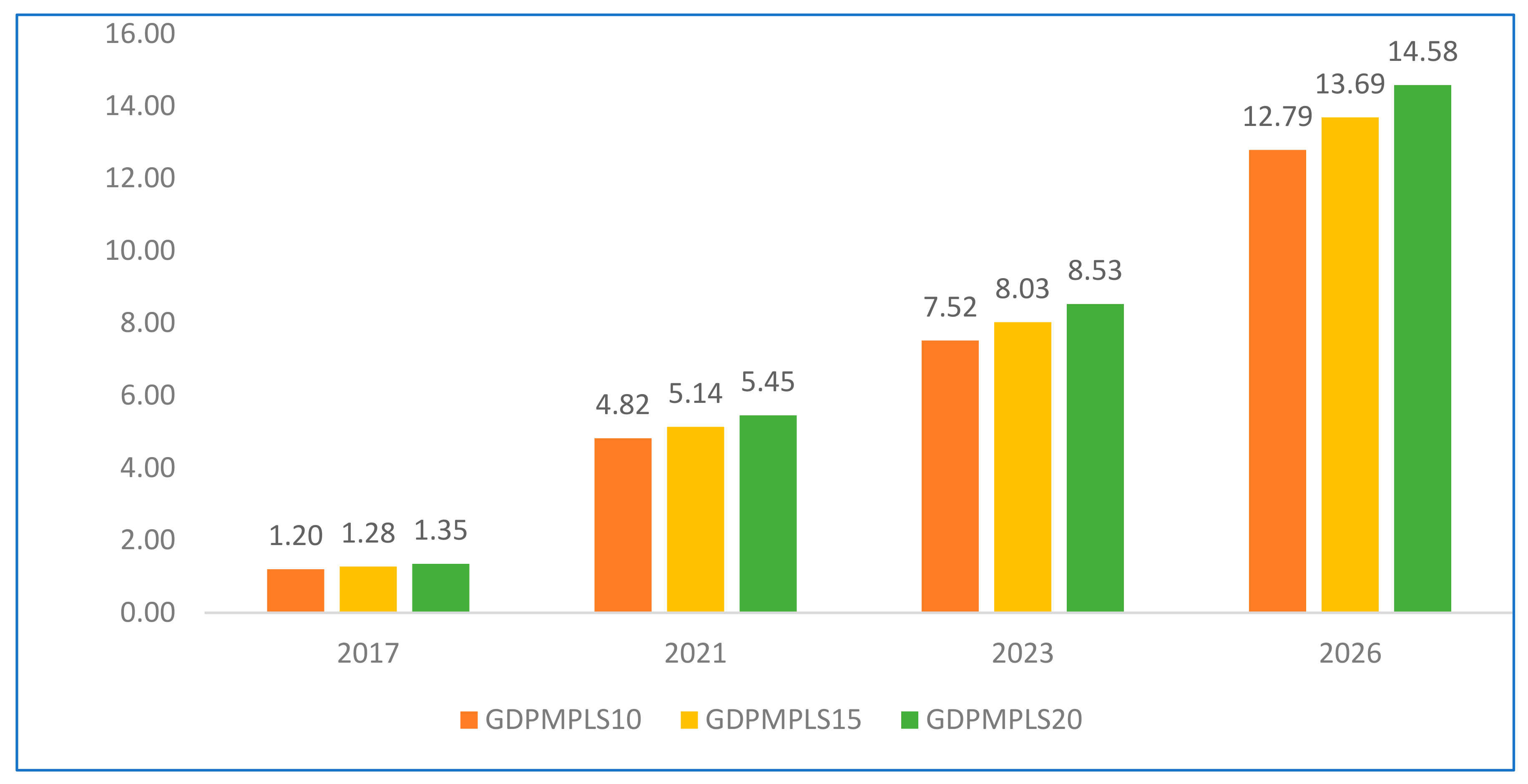
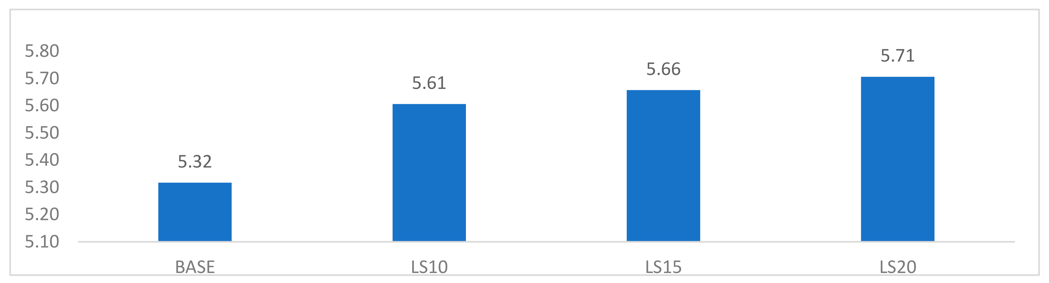
• The impact of an increase in the supply of skilled and semi-skilled labor under the LS20 simulation is greater than in the medium growth scenario (LS15) and other scenarios. This suggests that a higher proportion of skilled and semi-skilled workers will lead to a greater increase in aggregate productivity compared to a scenario with a low proportion of skilled and semi-skilled workers.
• The expansion of skilled and semi-skilled labor supply will have limited economic effects in the earlier periods, as it takes time for productivity improvements to have a widespread impact on the economy. This is because the productivity of skilled and semi-skilled labor affects the economy after a few years of workers’ engagement, which is consistent with the learning-by-doing growth hypothesis of endogenous growth theory.

Figure 4. Change in GDP (% change from BAU). Source: Model simulation results based on PSI-EU-SAM.

Figure 4. Change in GDP (% change from BAU). Source: Model simulation results based on PSI-EU-SAM.

4.1.2. Impact on Sectoral Output

The major effects of different skilled and semi-skilled labor supply shocks on the resulting sectoral compositions are outlined in

Table 7. Simulation results of sectoral output growth.

Sector	BAU	LS10	LS15	LS20	% Change from BAU
					LS10	LS15	LS20
Agriculture	5.42	5.51	5.54	5.58	0.09	0.13	0.16
Industry	4.94	6.47	6.51	6.55	1.53	1.57	1.61
Services	4.54	5.47	5.52	5.58	0.93	0.99	1.04
Total VAD FC	5.02	5.76	5.81	5.86	0.74	0.79	0.84

Source: Model simulation results based on PSI-EU-SAM.

.

First, the agriculture sector experiences the lowest benefits across all scenarios. In the high growth scenario (LS20), the annual production of the agriculture sector only increases marginally by 0.16 percentage points compared to the BAU scenario. Similarly, in the medium growth scenario (LS15), the growth in the agriculture sector output is modest, with only a 0.13 percentage point increase compared to the BAU scenario. This increase is still lower than the impact on GDP. In other words, the impact on agriculture, in proportion, is lower than the impact on GDP. It is found in the literature that the impact of tertiary education on agricultural productivity can be insignificant and even negative, particularly (Reimers & Klasen, 2013). Our analysis shows that agriculture benefits less from skilled and semi-skilled labour compared to industry and service sectors, which are more knowledge-intensive. In addition to the above mentioned findings in the literature, this could be due to structural challenges that limit access to modern technology which requires higher level of education, such as very small land size which average land holding less than 1 hector per holder.

In the high growth scenario, the impact on GDP is on average 0.84 percentage points higher per annum compared to the BAU scenario. Similarly, in the medium growth scenario, the impact on GDP is 0.74 percentage points higher compared to the BAU scenario. In the low growth scenario (LS10), the impact on agricultural outputs is still minimal but positive, and much smaller than the impact on GDP. The reason for the low impact on agriculture in the simulation results is that the agriculture sector relies more on unskilled labor, whose supply is reduced as more workers migrate to the industry and services sectors following improved human capital development.

Second, although the contribution to GDP of the industry sector is still small, its role has been improving over time. Under the high growth scenario (PS20), the industry’s contribution to GDP is 1.61 percentage points higher than the BAU scenario. Similarly, under the medium growth scenario (LS15), the industry’s contribution increases by 1.57 percentage points compared to the BAU scenario. The impact on the services sector is also relatively better compared to agriculture in all scenarios. In the high growth scenario (LS20), the services sector grows by approximately 1.04 percentage points higher than the growth in the BAU scenario. In the medium growth scenario (LS15), the services sector grows by nearly 1.0 percentage point higher than the growth in the base case (BAU) scenario. Likewise, in the low growth scenario (LS10), the services sector grows by a margin of 0.93% compared to the growth under the BAU scenario, which is still higher than the impact on GDP. The higher impact on the industry sector is partly due to the moderate skill-intensive nature of manufacturing activities compared to agricultural activities. The same is true for the services sector.

4.1.3. Factor Income Effect

Table 8. Simulation results of factor income.

Annual Compounded Average % Changes from INITIAL
Labour Type	BASE	LS10	LS15	LS20
lab-n	4.53	4.26	4.31	4.36
lab-p	5.47	4.29	4.30	4.30
lab-s	5.47	4.98	4.97	4.97
lab-t	1.35	3.91	3.83	3.75
Capital Land Rural	6.17	6.8	6.86	6.92
Capital Livst Rural	5.61	5.72	5.78	5.83
Non-Agg-capital	4.86	2.88	2.94	3.00

Source: Model simulation results based on PSI-EU-SAM.

presents the impact of different scenarios on employment income in the country. The scenarios demonstrate a decrease in income share for unskilled and semi-skilled labor by 2026, attributed to a decline in the supply of unskilled labor and an increase in the supply of skilled and semi-skilled labor. The annual compounded growth rates also indicate a decrease in wage income for these labor categories. However, the total income for skilled labor increases, despite a decrease in wage rates, due to a higher proportion of skilled labor being employed in the economy compared to the BAU scenario. The greatest increase in income for skilled labor is observed in the low growth (LS10) scenario, followed by the medium growth (LS15) scenario, possibly due to a moderate decline in wage rates in these scenarios.

Income from rural land and livestock shows a slight increase in all scenarios, with the highest increase in rental income observed in the high growth (LS20) scenario. This suggests that the productivity of land and livestock improves with the increase in skilled and semi-skilled labor supply. On the other hand, income from non-agricultural capital is lower in all scenarios compared to the BAU scenario. This may be attributed to the low marginal productivity of capital resulting from the sudden increase in supply of skilled and semi-skilled labor, without a corresponding increase in capital.

4.1.4. Impact on the Income of Government and Poor Households

Figure 5 illustrates that the change in government revenue, compared to the business as usual (BAU) scenario, exhibits an upward trend. Specifically, under the low growth (LS10) scenario, government revenue surpasses its BAU equivalent by 0.29%. While the agricultural sector may not be a primary source of direct tax revenue for the government, a surge in skilled and semi-skilled labor presents a significant opportunity. This is because these workers are typically employed in industries and services, which are generally easier and more efficient to tax than agriculture. Consequently, a shift towards a labor supply biased towards skilled individuals can result in a substantial increase in government tax revenue. In fact, in the 2015/16 period, tax revenue from agricultural income and rural land use fees accounted for only 0.04% of GDP (Mengistu et al., 2018). Consequently, it is noteworthy that government revenue experiences a marginal increase by augmenting the outputs of non-agricultural sectors.

A thorough analysis of the macro simulation results reveals a significant surge in imports and a decline in household consumption. Given that imports contribute significantly to tax revenue, the increase in imports has generated more tax revenue than the potential loss of revenue due to the decrease in domestic consumption. In simpler terms, the fiscal impact of the shock is reflected in the reduction of domestic tax revenues resulting from lower household consumption and the increase in international trade taxes from higher imports. This holds true across all scenarios, with the high growth (LS20) scenario generating more revenue compared to the others. This is because income in the BAU scenario is derived from self-employment, which is not subject to taxation. However, in the high growth (LS20) and medium growth (LS15) scenarios, increased income arises from formal sector employment, which is taxable due to productivity improvements.

Although it is interesting to understand the full extent of income distribution resulting from changes in labor utilization, it is particularly important to examine the impact on individuals living in poverty and the middle class (excluding those in the top 20%), as any change in their income can have significant consequences.

Table 9. Simulation results of income distribution by poverty household groups.

Annual Compound % Changes from INITIAL
Household Type	INITIAL	BASE	LS10	LS15	LS20
Rural poor	164.83	4.81	4.47	4.52	4.57
Rural middle class	529.38	4.67	4.25	4.30	4.34
Rural rich	162.03	4.44	4.04	4.07	4.10
Urban poor	19.96	4.00	3.36	3.40	3.43
Urban middle income	179.50	4.28	3.50	3.54	3.57
Urban rich	303.14	4.00	3.64	3.65	3.66

Source: Model simulation results based on PSI-EU-SAM.

presents the income distribution among different household groups in all scenarios. In comparison to the business as usual (BAU) scenario, income decreases for all types of households. However, in relation to the initial income level, rural households experience a slight increase in income compared to urban households.

To understand these patterns, it is important to note that the expansion of skilled and semi-skilled labor has a minimal impact on the income of those living in poverty, as they already lack skills. When considering the overall impact, the decline in income is significant in the low growth (LS10) scenario. In summary, it is worth noting that in all scenarios, the increase in skilled and semi-skilled labor supply shock has a negative impact compared to the business as usual (BAU) scenario.

5. Conclusions and Recommendations

We conducted a comprehensive analysis of the effect of human capital on the economy using the Computable General Equilibrium (CGE) model approach based on the Social Accounting Matrix (SAM) of PSI to investigate the impact of skill-biased labor supply shocks on the Ethiopian economy. We developed three plausible scenarios for CGE analysis: high growth (LS20) scenario, medium growth (LS15) scenario, and low growth (LS10) scenario. These scenarios were compared to a “Business As Usual” (BAU) scenario to assess the potential effects.

In the high growth (LS20) scenario, which models a 20% increase in skilled and semi-skilled labor supply, we observed substantial improvements in GDP, non-agricultural sector output, exports, fixed investments, imports, and net indirect tax. Similarly, the medium growth (LS15) scenario, assuming a 15% increase in skilled and semi-skilled labor supply, demonstrated positive impacts on growth indicators. Finally, the low growth (LS10) scenario, with a 10% increase in skilled and semi-skilled labor supply, allowed us to assess the economy-wide and sectoral output effects.

Our findings revealed four noteworthy results. Firstly, both GDP and non-agricultural sector output experienced significant growth in the high growth (LS20) and medium growth (LS15) scenarios, as well as in the low growth (LS10) scenario although the impact is minimal. Export performance, fixed investments, imports, and net indirect tax also showed promising improvements under these scenarios. Secondly, growth in these scenario surpassed that of the BAU scenario, indicating that skill-biased labor expansion has the potential to support further growth. This implies that there is room for growth before reaching a limit. Exports, gross fixed investments, imports, government revenue, and tax revenues substantially increased in these scenarios. Thirdly, the impact on poor households in the LS20 scenario was comparable to that of the BAU scenario, implying that this scenario yields minimal negative outcomes for these vulnerable groups. Lastly, we observed that the response to skill-biased labor supply shocks is not immediate. Instead, notable effects materialize several years after the implementation of the shock, which can be attributed to the time required to internalize the skills and knowledge of human capital. This finding aligns with the learning-by-doing growth hypothesis.

In conclusion, our study underscores the importance of human capital in driving economic growth. We highlight the potential benefits of skill-biased labor supply shocks and stress the time lag in experiencing their effects. These findings contribute to a deeper understanding of the role of human capital in economic development. The study concludes that implementing appropriate policy measures is crucial to stimulate the economy and optimize the allocation of available resources for sustainable economic growth. Failure to take immediate action will result in suboptimal outcomes with lasting impacts. Policies aimed at sustaining growth and efficiently utilizing abundant resources, such as labor, in developing countries should be evaluated not only for their immediate growth impact but also for future development. It is of utmost importance to align skills training and labor market demands to ensure that an excess supply of labor yields positive effects on the economy. As such, employment and education policies should be synchronized with the economy’s needs, and their effectiveness should be continuously monitored.

Based on the study’s findings, we recommend that governments:

• Invest in education and training to enhance the supply of skilled and semi-skilled labor, thus facilitating economic diversification beyond agriculture.
• Design educational programs that equip graduates with skills that are currently in demand in the labor market. This will improve employability and reduce skill mismatches.
• Regularly monitor education and employment policies to evaluate their effectiveness in aligning with the economy’s requirements, making adjustments as necessary.
• Expand financial inclusion to entrepreneurs and small businesses, enabling their growth and job creation, particularly in non-agricultural sectors where governments can collect increased tax revenues.

References

1. Acemoglu, D. (2009). Introduction to modern economic growth. Princeton University Press. [Google Scholar]
2. Acemoglu, D., Laibson, D., & John, A. L. (2019). Economics global edition. Pearson Education Limited. [Google Scholar]
3. Aghion, P., Antonin, C., & Bunel, S. (2021). Skill-biased technical change and economic growth. Journal of Economic Growth, 26(3), 275–310. [Google Scholar]
4. Ararat, L. O. (2009). The impact of human capital on economic growth: A case study in post-Soviet Ukraine, 1989–2009. Palgrave Macmillan. [Google Scholar]
5. Bahar, D., Choudhury, P., & Rapoport, H. (2020). Migration, innovation, and growth (World Bank Policy Research Working Paper No. 9287). World Bank Group. [Google Scholar]
6. Diao, X., Thurlow, J., & Benin, S. (2012). Strategies and priorities for African agriculture: Economy-wide perspectives from country studies. International Food Policy Research Institute. [Google Scholar]
7. Domar, E. (1946). Capital expansion, rate of growth, and employment. Econometrica, 14, 137–147. [Google Scholar] [CrossRef]
8. Dorosh, P., Robinson, S., & Ahmed, H. (2011). Economic implications of foreign exchange rationing in Ethiopia. Ethiopian Journal of Economics, 18, 132. [Google Scholar]
9. Federal Ministry of Education. (2021). Education Sector development programme VI (ESDP VI) 2013–2017 E.C. 2020/21–2024/25 G.C. Federal Democratic Republic of Ethiopia. [Google Scholar]
10. Harrod, R. F. (1939). An Essay in Dynamic Theory. The Economic Journal, 49, 14–33. [Google Scholar] [CrossRef]
11. International Food Policy Research Institute (IFPRI). (2011). Social accounting matrix for Ethiopia, 2011. IFPRI. [Google Scholar]
12. Klarin, T. (2018). The concept of sustainable development: From its beginning to the contemporary issues. Zagreb International Review of Economics and Business, 21(1), 67–94. [Google Scholar] [CrossRef]
13. Krishnan, P., & Shaorshadez, I. (2013). Technical and vocational education and training in Ethiopia (Working Paper for the International Growth Centre–Ethiopia Country Programme). International Growth Centre (IGC). [Google Scholar]
14. Lofgren, H., Harris, R. L., Robinson, S., Marcelle, T., & El-Said, M. (2002). A standard computable general equilibrium (CGE) model in GAMS. International Food Policy Research Institiute. [Google Scholar]
15. Manioudis, M., & Meramveliotakis, G. (2022). Broad strokes towards a grand theory in the analysis of sustainable development: A return to the classical political economy. New Political Economy, 27(5), 866–878. [Google Scholar] [CrossRef]
16. Mankiw, N. G., Romer, D., & Weil, D. N. (1992). A contribution to the empirics of economic growth. Quarterly Journal of Economics, 107, 407–437. [Google Scholar] [CrossRef]
17. Mengistu, A., Bekele, F., & Gedefe, K. (2018). Domestic resource mobilization in Ethiopia: Trends, causes, and prospects (Unpublished PSI Report). PSI.
18. Ministry of Finance. (2021–2022). Public expenditure data. Ministry of Finance. [Google Scholar]
19. National Bank of Ethiopia. (2021). Annual report 2020/21; National Bank of Ethiopia. Available online: https://nbe.gov.et/wp-content/uploads/2024/04/2020-21-Annual-Report-for-Publication.pdf (accessed on 11 December 2024).
20. Philippe, A., & Peter, H. (2009). The economics of growth. The MIT Press. [Google Scholar]
21. Policy Studies Institute-European Union (PSI-EU). (2016). Social accounting matrix. PSI-EU. [Google Scholar]
22. Pritchett, L. (2001). Where has all the education gone? The World Bank Economic Review, 15, 367–391. [Google Scholar] [CrossRef]
23. Reimers, M., & Klasen, S. (2013). Revisiting the role of education for agricultural productivity. American Journal of Agricultural Economics, 95(1), 131–152. [Google Scholar] [CrossRef]
24. Robert, J. B., & Xavier, S.-i.-M. (2004). Economic growth. The MIT Press. [Google Scholar]
25. Romer, D. (2019). Advanced macroeconomics (5th ed.). University of California. [Google Scholar]
26. Romer, P. M. (1990). Endogenous technological change: The problem of development. The Journal of Political Economy, 98, 71–101. [Google Scholar] [CrossRef]
27. Savvides, A., & Stengos, T. (2009). Human capital and economic growth. Stanford University Press. [Google Scholar]
28. Schmidt, E., & Woldeyes, F. (2019). Rural youth and employment in Ethiopia, youth and jobs in rural Africa (pp. 109–136). Oxford University Press. Available online: https://academic.oup.com/book/37379/chapter/331369233 (accessed on 13 January 2025).
29. Thurlow, J. (2008). A recursive dynamic CGE model and microsimulation poverty module for South Africa. International Food Policy Research Institute. [Google Scholar]
30. UNESCO. (2015). 2030—Incheon declaration and framework for action. Available online: https://unesdoc.unesco.org/ark:/48223/pf0000245656/Pdf/245656eng.pdf.multi (accessed on 24 December 2024).
31. United Nations. (2022). Statistical yearbook (2022 ed.). United Nations Department of Economic and Social Affairs, Statistics Division. Available online: https://desapublications.un.org/publications/statistical-yearbook-2022-edition (accessed on 24 December 2024).
32. Worku, M. Y. (2025). Access-equity tensions in education: Examining Ethiopia’s educational reforms through a distributive social justice lens. Social Sciences & Humanities Open, 11, 101443. [Google Scholar]
Figure 1. Education expenditure (% total government expenditure). Source: Ministry of Finance (2021–2022).
Economies 13 00137 g001
Figure 2. Education expenditure (% GDP). Source: Ministry of Finance (2021–2022).
Economies 13 00137 g002
Figure 3. Growth rates of per capita GDP and education expenditure. CGE Model Simulation Results and Discussion.
Economies 13 00137 g003
Figure 5. Government income (% change). Source: Model simulation results based on PSI-EU-SAM.
Economies 13 00137 g005