Money Demand in Indonesia and Its Forecasting to 2033

Abstract

This study aims to identify the primary factors influencing the demand for money in Indonesia and to provide forecasts through 2033. The research employs two methodologies: time series econometrics and machine learning, utilizing data spanning from the first quarter of 2010 (2010Q1) to the fourth quarter of 2023 (2023Q4). The results of the study indicate that, in the long term, the demand for money in Indonesia is influenced by two main determinants: Gross Domestic Product (GDP) and Financial Institution Depth (FID). In the short term, the significant determinants include interest rates, inflation rates, GDP lag, FID lag, and electricity access. The forecast results suggest that the demand for money in Indonesia is projected to experience positive growth, reaching IDR 16,855,845 billion by 2033. This finding underscores the continued importance of physical currency in the Indonesian economy. Based on these results, this study serves as a guideline for policymakers in managing the demand for money by considering the variables that can either increase or decrease this demand. The positive forecast for the demand for money also highlights its significant role in supporting a stable Indonesian economy in the future.

1. Introduction

Issues related to the demand for money in a country are crucial for policymakers, particularly the central bank, in maintaining the stability of economic growth from a monetary perspective (Baharumshah et al., 2009). However, the demand for money is difficult to predict due to changes in consumer and business behavior regarding the use of money, particularly banknotes and coins. This situation requires regulatory adjustments in response to these behavioral changes, which have implications for the instability of money demand within a country (Lucas & Nicolini, 2015). Indonesia, as one of the developing countries, is facing challenges related to the stability of money demand. Economic developments, along with changes in consumer and business behavior, have an impact on money circulation in Indonesia. Statistical data indicate that the demand for both paper money and deposits has continued to increase over the past decade. Figure 1 illustrates that the demand for banknotes and coins continues to increase along with the growth in demand for deposits, highlighting the importance of sustainable cash payments within the economy. In contrast, the growth rate of banknotes in Indonesia indicates a fluctuating trend, with the highest growth observed in 2020, likely influenced by specific economic or social factors during that period. This trend underscores the dynamic nature of cash usage in response to changing economic conditions and preferences due to various determinants and the importance of monitoring money movements from a currency demand perspective to ensure an efficient payment system. Therefore, it highlights that predictions related to money demand are a critical aspect that can support economic stability, particularly in Indonesia, which is currently experiencing fluctuations in money demand. The development of studies related to money demand has been an important concern for researchers, particularly in the context of specific countries over the past decade (Asiedu et al., 2021; Bahmani-Oskooee & Bahmani, 2015; Ben-Salha & Jaidi, 2014; Dou, 2018; Mera & Pop Silaghi, 2018; Opoku, 2017). This is closely related to the important role of money as the center of modern economic development, as it fosters public confidence in economic value (McLeay et al., 2014). The magnitude of a country’s money demand has a causal relationship with its macroeconomic indicators, which are often measured by GDP, inequality, and inflation (Adil et al., 2022; Hicham, 2020; Khan et al., 2021; Stylianou et al., 2024). The stability of money demand is one of the main objectives of monetary policy, although the growth of money demand is frequently associated with an increase in a country’s macroeconomic indicators (Achsani, 2010; Nel et al., 2020). To ensure the effective implementation of a country’s monetary policy, it is important to analyze the factors that influence money demand. However, the existing literature primarily focuses on the determinants of money demand and often neglects the development of predictive models for future monetary needs.

Therefore, this study aims to address this gap by predicting the trend of money demand. To achieve this objective, the determinant factors must be examined as key drivers of future money demand movements. The predictions could assist policymakers, particularly the central bank and the printing industry, in estimating the appropriate value of money demand, thereby maintaining economic stability.

Based on the issues related to the demand for money in Indonesia, which continues to fluctuate annually, this study seeks to address how money demand will evolve in the future: will it continue to increase or decrease? By predicting the demand for money in Indonesia, policymakers will have a direction in determining appropriate monetary policies to maintain the stability of the Indonesian economy and to promote financial inclusion, particularly in areas with limited access to digital financial services. On the other hand, the money printing industry also has a future direction for synergy with the central bank, including the procurement and printing of banknotes as well as waste management within this sector (Bahri et al., 2022). This is particularly relevant in Indonesia, where the majority of the population still relies on cash transactions, although the adoption of digital payments is increasing in urban areas. In conclusion, the development of a reliable model to forecast the amount of money in circulation is essential for effective monetary planning and inclusive financial development. This study specifically focuses on M1 (narrow money) due to the prevalent use of banknotes and coins in Indonesia. Furthermore, forecasting Indonesian money demand until 2033 could assist policymakers in formulating appropriate monetary policies to stabilize the Indonesian monetary system and promote economic growth.

The structure of this article is as follows: Section 1 provides an introduction that outlines the problem addressed in this study. Section 2 presents a literature review, highlighting relevant theories and previous findings related to the demand for money. Section 3 describes the methodology used, including research materials and analytical techniques. Section 4 and Section 5 discuss the results and provide comparisons with previous studies. Finally, Section 6 concludes the article by summarizing the main findings and offering managerial implications and limitations of the study.

2. Literature Review

Several key theories explain the development of the determinants of money demand. According to Fisher (1911), the demand for money is influenced by the level of nominal income. Meanwhile, Keynes (1936) argued that the demand for money depends on both the level of nominal income and interest rates. Friedman (1956) proposes that the determinants of money demand in a country can be influenced by three factors: the level of income, interest rates, and inflation expectations, which reflect the elasticity of income with respect to money demand. In addition, Baumol (1952) and Tobin (1958) revealed that the liquidity preference for assets with high expected returns, a theoretical approach to the money demand model in terms of cash management and the storage of other assets, can be considered a determinant of a country’s money demand, alongside the three previously mentioned factors. Furthermore, Mundell (1963) posited that the exchange rate is a primary determinant, in addition to income and interest rates. The development of payment systems based on credit cards, debit cards, and ATMs could also be regarded as a significant factor in determining money demand (Boeschoten, 1998). Therefore, the issue of financial innovation is an essential consideration, as the exclusion of this factor may lead to misspecification in the analysis (Arrau et al., 1995).

Several previous studies have examined the factors influencing the demand for money through various case studies of countries in recent years. A previous study by Farazmand and Moradi (2015) analyzed the determinants of money demand in several Middle Eastern countries from 1980 to 2013 using the autoregressive distributed lag (ARDL) approach. Their analysis revealed that inflation and exchange rates had a negative effect on money demand, while income exhibited a positive and significant effect. Aggarwal (2016) analyzed the determinants of money demand in India using cointegration and regression tests with the ordinary least squares (OLS) approach from 1996 to 2013 with quarterly data. The results of the study indicated that there was no long-term relationship between the independent and dependent variables. Furthermore, the OLS analysis revealed that GDP and interest rates positively affected money demand in the short term, specifically in the case of M1. Opoku (2017) analyzed the determinants of money demand in Ghana using the autoregressive distributed lag (ARDL) approach from 1970 to 2012. His analysis found that inflation and interest rates had a negative effect on money demand in both the short and long term. In contrast, financial innovation, as proxied by the M2/M1 ratio, exhibited a negative and significant effect only in the short term. In his study, the exchange rate was found to have a positive and significant effect in the short term. Dou (2018) analyzed the determinants of money demand in China using linear econometric models and structural vector autoregression (SVAR) from 1996 to 2016. His empirical results indicated that income, interest rates, and inflation expectations significantly influenced China’s money demand. Additionally, financial innovation, government debt, capital mobility, and exchange rate substitution played a minor role in the demand for broad money. Asiedu et al. (2021) analyzed the demand for long-term money in 16 West African countries using the autoregressive distributed lag (ARDL) approach from 1982 to 2019. The results indicated that income levels had a positive and significant effect on money demand. However, in this context, LIBOR and foreign interest rates negatively affected the demand for money across the 16 countries.

In the Indonesian context, several previous studies have been conducted; however, the attention given to identifying the determinants is still limited. James (2005) found that financial liberalization is the key driver towards money demand and its fluctuation in Indonesia. Hossain (2007) also investigated the demand for narrow money in Indonesia from 1970 to 2005 by using regression analysis and found that the real income, inflation, and the return towards foreign financial assets had a significant impact on the narrow money demand. Wijaya et al. (2022) analyzed the drivers of money demand in Indonesia from 2006 to 2020 by applying the error correction model (ECM) and showed that the GDP and exchange rate have a positive impact on the Indonesian money demand, while deposit rates have a negative effect. Fatihah and Pasaribu (2024) examined the determinant factors affecting money demand in Indonesia (M2) by using ECM from 2018 to 2023. The result found that the interest rates and the US dollar exchange to rupiah are the factors influencing Indonesian money demand (M2).

Based on some previous findings, the variation of key drivers still relies on the macroeconomic factor, which means that the improvement of the money demand model must be implemented by adding an additional variable. On the other hand, several previous studies have explored the prediction of money demand in various countries. These studies commonly employ econometric methods to analyze the demand for money in order to identify the driving factors and make future predictions, especially in ECM analysis. In Indonesia, the fluctuations in money demand could provide valuable insights for advancing knowledge in this area. On the other hand, the novel contribution of this study, compared to other research related to the case in Indonesia, is the application of machine learning as a predictive tool for money demand, providing alternative predictions that can be utilized by policymakers. The combination of econometric methods and machine learning results in a range of alternative predictions that can be considered by policymakers. Therefore, this study aims to address the research gap by focusing on the specific context of Indonesian money demand growth and its implications for monetary policy and economic planning.

3. Methodology

This study employs an econometric model to achieve its objectives, drawing on established theories regarding the determinants of money demand. Key factors considered include income levels, interest rates, inflation, exchange rates, liquidity preferences, and advancements in payment system technology. Narrow money (M1) is utilized as an indicator of money demand, focusing on the predicted demand for physical currency in circulation, such as banknotes and coins. According to some previous studies, there are several variables that can be adopted in this analysis, including economic indicators such as GDP, interest rates, inflation, and exchange rates, as well as a technology indicator. Additionally, the development of digital payment systems influences the factors determining money demand in the future. Therefore, we include a variable representing the percentage of the population with access to electricity as a factor affecting money demand. The ease of accessing electricity can impact the money supply to GDP ratio (Owolabi et al., 2021). Therefore, the model for predicting money demand in Indonesia is as follows:

MD = f(GDP, IR, FID, AEL, INF, EXR)

(1)

where MD is the narrow money demand (M1), which refers to the demand for banknotes and coins. GDP is the real income level, IR is the interest rate of the central bank in Indonesia, FID is the Indonesian financial institution index, AEL is the percentage of the population that can access electricity in Indonesia, INF is the inflation rate in Indonesia, and EXR is the nominal exchange rate. The function can be written in a log-linear form, as follows:

LnMDt = B₀ +B₁LnGDPt + B₂IRt + B₃FIDt + B₄AELt + B₅INFt + B₆LnEXRt + e_t

(2)

where Ln is the natural logarithm, B₀ is a constant, while B₁-B₆ are the coefficients of each variable, and e_t is the error rate that explains other factors determining money demand that cannot be explained in the model.

The analysis in this study comprises several steps, which include the following:

• Pre-processing data

Data pre-processing ensures readiness for analysis, with disaggregation converting annual data into higher-frequency formats (e.g., quarterly) to meet specific analytical needs. Utilizing the Chow-Lin method, this process employed regression with auxiliary variables to distribute data consistently while preserving its original dynamics, thereby supporting high-resolution analyses such as trend or economic cycle studies.

2.

Time Series Data Decomposition

This study employed decomposition prior to conducting the regression analysis, using the Hodrick–Prescott (HP) filter as one of the statistical methods for decomposing time series data into a long-term trend component and a short-term cyclical component. This method is commonly used in economic analysis to identify fundamental trends. By minimizing a loss function that balances the fit to actual data with trend smoothness, the HP filter adjusts the smoothing parameter (λ) based on data frequency (e.g., 100 for annual data, 1600 for quarterly data, and 14,400 for monthly data).

3.

Estimating and Forecasting Analysis

This study employed two analytical approaches for estimation and forecasting: time series analysis and machine learning, ensuring comprehensive results. The time series approach used the error correction model (ECM) to examine long-term relationships and short-term adjustments in non-stationary data, as well as the autoregressive distributed lag (ARDL) method to analyze both short- and long-term dynamics without requiring all variables to be stationary at the same level. In this approach, the study also employed the series integrated at the first difference and had cointegration among the variables. Consequently, lagged variables were implemented to capture both short-run and long-run dynamics, as derived from Equations (2) and (3) as follows:

ΔLnMD_t = λ₀ + θ₀LnMD_t−1 + ΣB1ΔLnGDP_t−i + ΣB2ΔIR_t−i + ΣB3ΔFID_t−i + ΣB4ΔAEL_t−i + ΣB₅ΔINF_t−i + ΣB6ΔLnEXR_t−i + ϕ ECM_t−1 + e_t

(3)

Machine learning methods, on the other hand, were used to capture complex, non-linear patterns in data. Techniques include random forest (RF), an ensemble-based method that enhances prediction accuracy; multivariate adaptive regression spline (MARS), which flexibly captures non-linear relationships and interactions; and support vector machine-linear (SVM-Lin), designed for robust predictions in linear data. This combined approach provides an in-depth analysis of dynamic variable relationships while uncovering patterns beyond those identified by traditional methods. Additionally, this study also employed univariate methods to forecast Indonesian money demand.

The data for this study were collected from various sources covering the period from 2010Q1 to 2023Q4. The source for money demand (MD) or M1 and interest rates (IR) was the Central Bank of Indonesia. GDP and inflation (INF) data were obtained from Statistics Indonesia. The financial institution index (FID) was collected from the International Monetary Fund (IMF), while access to electricity (AEL) and the exchange rate (EXR) data were gathered from World Bank Open Data and Investing.com. A summary of these variables is presented in

Table 1. The operational definitions of the variables.

Notation	Description	Unit	Source
MDt	Money demand proxied by currency products, such as banknotes and coin outside commercial and rural banks	IDR	Central Bank of Indonesia (BI)
GDPt	Gross Domestic Product (GDP) in constant based on expenditure (2010)	IDR	Statistics Indonesia
IRt	Central Bank of Indonesia (BI) Rate	%	Central Bank of Indonesia (BI)
FIDt	Financial Institution Index	-	International Monetary Fund (IMF)
AELt	Access to Electricity (% of population)	%	World Bank Open Data
INFt	Inflation rate in Indonesia, using 2018 as the base year	%	Statistics Indonesia
EXRt	The nominal exchange rate from IDR to USD	IDR/USD	Investing.Com

.

4. Results

Before estimating the determinants of money demand in Indonesia, the results of the stationarity test as an initial step in the analysis are presented in

Table 2. Stationary test.

Variable	Test Equation	Level		First-Difference
		ADF	p-Value	ADF	p-Value
MDt	Trend and Intercept	−1.587	0.786	−6.394	0.000 **
	Intercept	−3.448	0.013 **	−0.852	0.796
	None	0.303	0.770	−1.259	0.189
GDPt	Trend and Intercept	−2.145	0.510	−3.080	0.075
	Intercept	−1.150	0.689	−3.218	0.024 **
	None	2.812	0.999	−1.408	0.147
Irt	Trend and Intercept	−2.072	0.550	−4.772	0.002 **
	Intercept	−1.988	0.291	−4.772	0.000 **
	None	−0.439	0.520	−4.817	0.000 **
FIDt	Trend and Intercept	−2.912	0.167	−6.408	0.000 **
	Intercept	−1.770	0.392	−6.417	0.000 **
	None	3.685	1.000	−5.343	0.000 **
AELt	Trend and Intercept	0.266	0.998	−3.443	0.058 *
	Intercept	−2.339	0.164	−2.086	0.251
	None	1.273	0.947	−1.750	0.076 *
INFt	Trend and Intercept	−2.763	0.217	−2.884	0.176
	Intercept	−2.018	0.278	−2.899	0.053 *
	None	−1.017	0.274	−2.910	0.004 **
EXRt	Trend and Intercept	−1.063	0.926	−5.823	0.000 **
	Intercept	−1.529	0.512	−5.708	0.000 **
	None	2.311	0.995	−4.643	0.000 **

Notes: ** significant at 5% level of significance; * significant at 10% level of significance.

. Data are considered stationary if it does not exhibit a specific movement pattern, such as a trend. In other words, stationary data does not display a consistent upward or downward direction over time. A series is deemed stationary if it has a constant mean, constant variance, and constant covariance across various lags. This study employed the augmented Dickey–Fuller (ADF) unit root test to assess data stationarity, both at the level and the first difference. The level refers to the initial value without transformation or absolute adjustment, while the first difference represents the change between a specific period and the preceding period. Stationarity can also be determined based on the probability value; if the probability value is less than the 5% significance level, the data are considered stationary. The results of the ADF unit root test indicate that all variables are stationary at the first difference with a significance level of 5%, except for the electricity variable, which is significant at the 10% level. This finding is corroborated by the probability values for each observation (see Table 2). Furthermore, based on McKinnon’s critical values, all variables examined in this study are stationary at the significance levels of 1%, 5%, and 10%. Following the stationary analysis, this study predicted money demand in Indonesia using the error correction model (ECM) and the autoregressive distributed lag (ARDL) approach. The selection of the optimal model is based on evaluation criteria such as adjusted R-squared (R² adj), which assesses the model’s accuracy in explaining the dependent variable while accounting for the number of independent variables, and the Akaike information criterion (AIC), which identifies the model that achieves the best balance between goodness-of-fit and complexity. The combination of these criteria ensures that the selected model is not only accurate but also efficient in elucidating the relationships between variables.

In the first estimation (ECM) presented in

Table 3. ECM for money demand prediction.

Variable	Coefficient	Std. Error	t-Statistic	Prob.
C	−6.8843	2.0032	−3.4367	0.0014 **
MD(-1)	−0.5748	0.1213	−4.7390	0.0000 **
IR(-1)	−0.0088	0.0079	−1.1151	0.2713
INF(-1)	0.0014	0.0062	0.2236	0.8242
GDP(-1)	1.0472	0.2688	3.8960	0.0004 **
FID(-1)	4.3351	1.8568	2.3347	0.0245 **
EXR(-1)	−0.1029	0.1103	−0.9326	0.3565
AEL(-1)	0.0007	0.0142	0.0470	0.9628
D(IR)	0.0353	0.0150	2.3515	0.0236 **
D(INF)	−0.0099	0.0074	−1.3426	0.1868
D(GDP)	1.0198	0.2708	3.7656	0.0005 **
D(FID)	6.0626	3.1038	1.9533	0.0576 *
D(EXR)	0.0823	0.2333	0.3528	0.7260
D(AEL)	−0.0523	0.0285	−1.8395	0.0731 *

Notes: ** significant at 5% level of significance; * significant at 10% level of significance.

, the results indicate that the variables MD(-1), GDP(-1), FID(-1), D(IR), D(GDP), and D(FID) significantly influence money demand (MD). The variable MD(-1) exhibits a negative coefficient of −0.5748, suggesting that money demand in the previous period is inversely related to current money demand, with high significance (Prob. = 0.0000). This finding implies that an increase in money demand in the previous period tends to reduce money demand in the subsequent period, potentially reflecting a correction mechanism within the monetary system aimed at maintaining equilibrium in money circulation. Conversely, GDP(-1) and FID(-1) show a significant positive relationship with money demand (MD), with coefficients of 1.0472 and 4.3351, respectively. This indicates that economic growth (GDP) and the depth of financial institutions (FID) in the previous period enhance money demand in the current period, reflecting that economic activities and financial sector development support an increase in money demand. Additionally, changes in GDP (D(GDP)) and FID (D(FID)) also have a significant positive impact on MD, with coefficients of 1.0198 and 6.0626, respectively.

This suggests that economic growth and the deepening of financial institutions directly contribute to an increase in money demand. Additionally, changes in interest rates (D(IR)) exhibit a significant positive relationship, with a coefficient of 0.0353 (Prob. = 0.0236). This indicates that a short-term rise in interest rates may be associated with increased money demand, potentially due to shifts in market behavior or investment flows.

However, some variables, such as IR(-1), INF(-1), and EXR(-1), are not significant in the model, although they exhibit certain directional relationships. The negative coefficients for IR(-1) and EXR(-1) indicate that an increase in interest rates or a depreciation of the exchange rate in the previous period tends to reduce money demand, while inflation (INF(-1)) shows a weak positive relationship. Overall, this model indicates that economic factors such as GDP and FID, both in lagged and differenced forms, play a major role in influencing MD. Positive relationships suggest that increases in these factors drive money demand growth, while negative relationships reflect correction mechanisms or pressures that reduce money demand to maintain economic stability.

In the second analysis using the ARDL approach, several variables have different estimations compared to the ECM results (see

Table 4. ARDL for money demand prediction.

Variable	Coefficient	Std. Error	t-Statistic	Prob.
C	−5.7235	3.0789	−1.8589	0.0753 *
MD(-1) *	−0.4939	0.1715	−2.8794	0.0082 **
IR(-1)	−0.0029	0.0100	−0.2888	0.7752
INF(-1)	0.0055	0.0066	0.8287	0.4155
GDP(-1)	1.0251	0.4331	2.3670	0.0263 **
FID(-1)	4.7582	2.1819	2.1807	0.0392 **
EXR(-1)	−0.1629	0.1145	−1.4228	0.1677
AEL(-1)	−0.0143	0.0173	−0.8280	0.4158
D(MD(-1))	−0.3362	0.2213	−1.5194	0.1417
D(MD(-2))	−0.0227	0.2195	−0.1035	0.9184
D(MD(-3))	−0.3728	0.1460	−2.5542	0.0174 **
D(IR)	0.0267	0.0137	1.9531	0.0626 *
D(IR(-1))	0.0259	0.0111	2.3294	0.0286 **
D(INF)	−0.0130	0.0053	−2.4513	0.0219 **
D(INF(-1))	−0.0117	0.0059	−2.0012	0.0568 *
D(INF(-2))	0.0081	0.0050	1.6439	0.1132
D(GDP)	0.0322	0.2890	0.1115	0.9122
D(GDP(-1))	−0.9787	0.5695	−1.7187	0.0985 *
D(GDP(-2))	−1.3644	0.5377	−2.5375	0.0181 **
D(GDP(-3))	−1.0058	0.5081	−1.9796	0.0593 *
D(FID)	−3.4926	3.6760	−0.9501	0.3515
D(FID(-1))	−2.7531	2.6798	−1.0274	0.3145
D(FID(-2))	4.3983	2.1814	2.0163	0.0551 *
D(FID(-3))	2.6853	2.2879	1.1737	0.2520
D(EXR)	0.2855	0.1977	1.4439	0.1617
D(EXR(-1))	−0.3276	0.1708	−1.9187	0.0670 *
D(AEL)	−0.0591	0.0338	−1.7465	0.0935 *
D(AEL(-1))	−0.0629	0.0338	−1.8601	0.0752 *

Notes: ** significant at 5% level of significance; * significant at 10% level of significance.

). Based on the selection of optimal lags using the Akaike information criterion (AIC), the best model identified is ARDL (4, 2, 3, 4, 4, 2, 2). This indicates that the lags employed for each independent variable have been optimized to produce a model that achieves the best balance between accuracy (goodness-of-fit) and complexity. This diverse selection of lags enables the model to more accurately capture the dynamics of the temporal relationships between variables, both in the short and long term. Furthermore, this model reflects the flexibility of the ARDL approach in accommodating variables with varying levels of stationarity, thereby providing more reliable estimation results.

Based on Table 4, the estimation results of the ARDL model with the error correction model (ECM) provide valuable insights into the short-term and long-term factors influencing money demand (MD). In the long term, the significant negative coefficient of MD(-1) (−0.4939) highlights a correction mechanism that adjusts approximately 49.39% of any imbalance per period, ensuring stability in MD. Economic growth (GDP) and financial institution depth (FID) play a crucial role in driving MD. The positive coefficient for GDP(-1) (1.0251) suggests that strong economic growth in the past significantly increased MD by boosting economic activity and liquidity. Similarly, the positive coefficient of FID(-1) (4.7582) indicates that financial development, including increased credit access and financial services, enhances MD over time. In the short term, dynamic changes in variables such as interest rates, inflation, economic growth, and financial development significantly impact money demand (MD). Rising interest rates (D(IR): 0.0267) temporarily increase MD as markets shift toward higher-yield instruments. Conversely, inflation (D(INF): −0.0130) reduces MD by diminishing purchasing power and cash demand. Past economic growth (D(GDP(-2)): −1.3644) negatively affects current MD, reflecting a lagged effect where prior activity generated sufficient liquidity, reducing current demand. Financial development in earlier periods (D(FID(-2)): 4.3983) stimulates MD, while increased electricity access (D(AEL(-1)): −0.0629) reduces MD, possibly due to a shift toward digital transactions. Overall, the findings reveal the interplay of economic growth, financial development, and systemic adjustments in shaping MD, highlighting the growing impact of digital transformation. In this study, model evaluation was conducted through two key aspects: the classical assumption test and parameter stability. A robust model is one that satisfies the classical assumption test, which requires that the residuals exhibit no autocorrelation, have homoscedastic variance, and follow a normal distribution.

As shown in

Table 5. Model evaluation for Indonesian money demand.

Model	Adj R-Squared	AIC	Classical Assumption Test			Stability
			Autocorrelation	Heteroskedasticity	Normality	CUSUM
ECM	0.9928	−3.7138	✓	✓	✓	Stable
ARDL with ECM	0.9062	−4.9491	✓	✓	✓	Stable

✓ = The model has passed the classical assumption test.

, both models meet these classical assumptions for the residuals. The second aspect of evaluation focuses on parameter stability, assessed using the CUSUM test. The results indicate that both models utilized in this study demonstrate stable parameters. Furthermore, based on the adjusted R-squared criterion, the ECM model is identified as the best predictive model for MD. Forecasting is the subsequent step in this analysis following the selection of the optimal model for the determinants of money demand. Several machine learning methods are employed, including random forest (RF), multivariate adaptive regression spline (MARS), and support vector machine-linear (SVM-Lin).

Each method will be checked for goodness-of-fit measures (such as root mean square error (RMSE), R-squared, and mean absolute error (MAE)) to determine the best method to be used as a prediction model. The results of the model accuracy evaluation presented in

Table 6. The machine learning forecasting evaluation.

Dependent Variable	Method	R-Squared	RMSE	MAE
MD	RF	0.9544	0.1005	0.0691
	MARS	0.9883	0.0489	0.0381
	SVMlin	0.9890	0.0462	0.0340

compare the performance of three machine learning methods, random forest (RF), multivariate adaptive regression splines (MARS), and support vector machine with linear kernel (SVM-Lin), in predicting money demand (MD) and Peruri orders. For the MD variable, the SVM-Lin method achieves the best performance, with an R-squared value of 0.9890, indicating that 98.90% of the variation in MD is explained by the model.

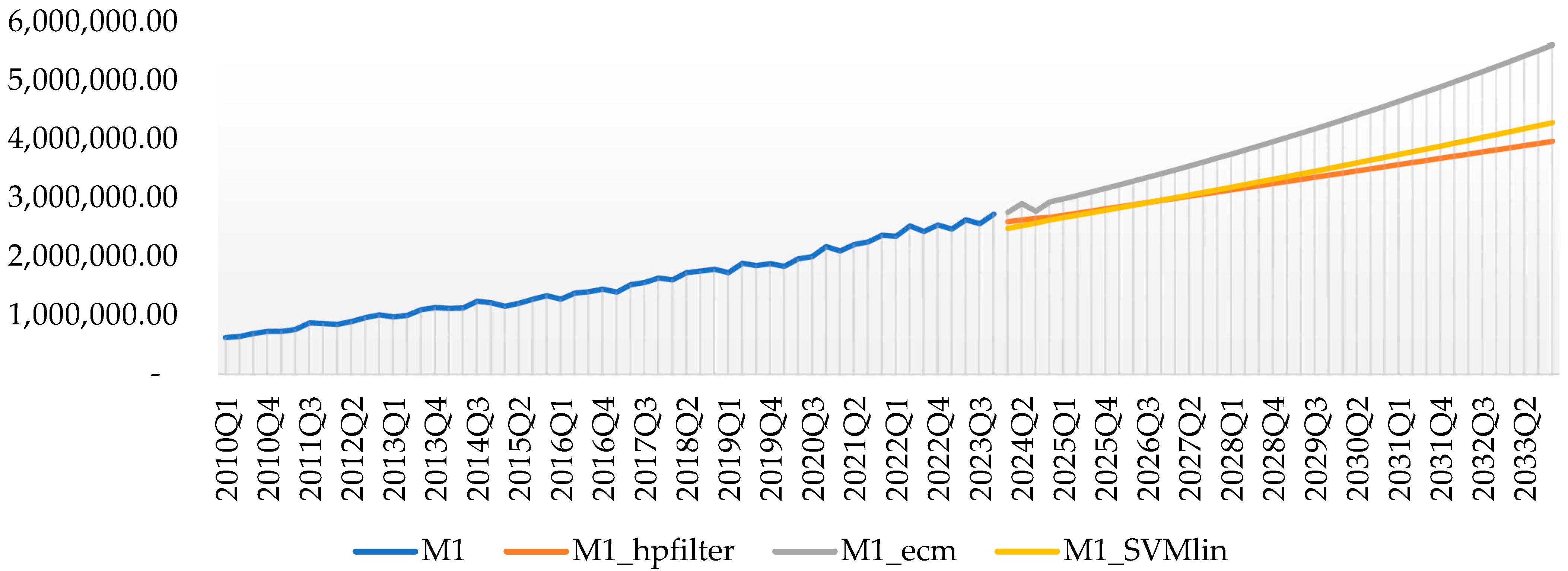
Furthermore, this method has the lowest error values, with an RMSE (root mean square error) of 0.0462 and MAE (mean absolute error) of 0.0340, making it the most accurate and efficient for predicting MD. Although MARS demonstrates comparable accuracy with an R-squared of 0.9883, RMSE of 0.0489, and MAE of 0.0381. Overall, SVMlin is identified as the best method for predicting MD due to its superior accuracy and lower error values compared to the other methods. The prediction results for MD using three methods—the univariate model (HP filter), error correction model (ECM), and SVMlin—show significant differences in projection patterns (Figure 2). The HP filter provides a stable and conservative trend, as represented by the orange line in the graph.

The ECM method, represented by the grey line, produces more aggressive projections, showing a sharp increase in MD after the historical data period. ECM captures long-term relationships and short-term adjustments among economic variables, making it responsive to structural changes. However, its RMSE value of 0.2275 indicates a higher error rate, suggesting lower accuracy despite its aggressive projections. In contrast, the SVMlin method offers a moderate projection, represented by the yellow line, which follows the historical trend of MD while showing higher growth than the HP filter. As a machine learning approach, SVMlin captures non-linear data patterns, balancing sensitivity to historical dynamics with flexibility to accommodate complex relationships. Its RMSE value of 0.04618 is much lower than ECM, indicating superior accuracy and smaller error rates. The results of the MD variable projection table (in billion rupiah) for 2024 to 2033 using three methods—univariate (HP filter), ECM, and SVMlin—reveal distinct growth patterns (Figure 2 for trend and

Table 7. Forecasting of Indonesian money demand period from 2024 to 2033 (in billion IDR).

Year	Univariate	ECM	SVMlin
2024	10,577,466.39	11,398,801.00	10,236,912.96
2025	11,070,158.61	12,329,692.20	10,942,684.31
2026	11,645,341.29	13,308,309.59	11,623,410.95
2027	12,220,523.98	14,348,066.92	12,321,458.27
2028	12,795,706.67	15,446,140.21	13,036,513.30
2029	13,370,889.36	16,604,810.80	13,768,235.21
2030	13,946,072.05	17,826,645.34	14,516,374.62
2031	14,521,254.74	19,114,317.07	15,280,554.06
2032	15,096,437.43	20,470,602.02	16,060,498.39
2033	15,671,620.12	21,898,381.89	16,855,844.55

Source: author calculation (2024).

for statistical results).

The univariate (HP filter) method offers a conservative and stable projection, with MD values gradually increasing from IDR 10,577,466 billion in 2024 to IDR 15,671,620 billion in 2033. This method relies solely on historical trend patterns, resulting in a linear and lower projection compared to other methods. In contrast, the ECM method provides a more aggressive projection, with MD values expected to rise from IDR 11,398,801 billion in 2024 to IDR 21,898,382 billion in 2033. The ECM model predicts a significant acceleration in MD growth, reflecting anticipated major changes in economic factors affecting MD. However, this projection carries a higher risk of overestimation, as indicated by its higher error rate compared to the machine learning method. The SVMlin method, on the other hand, produces a more moderate and realistic projection than ECM, with MD values projected to increase from IDR 10,236,913 billion in 2024 to IDR 16,855,845 billion in 2033. This method effectively captures complex data patterns and demonstrates the lowest error rate, indicating better accuracy than the other methods. Overall, the univariate method provides the most conservative projection, while the ECM method offers an optimistic projection with faster growth. However, the SVMlin method delivers the most realistic and accurate results, striking a balance between sensitivity to historical patterns and the ability to capture complex dynamics. Therefore, SVM-Lin is identified as the optimal method for projecting money demand (MD) during the period from 2024 to 2033.

5. Discussion

The results of this study indicate that the demand for money in Indonesia is influenced by several factors. Both GDP and financial institution depth (FID) have long-term effects on money demand, while interest rates (IR), inflation (INF), lagged GDP, FID, and access to electricity (AEL) affect money demand in the short term. We found that only two factors significantly influence a country’s money demand in both the short and long term. This finding reinforces previous research, which has revealed that GDP is a crucial determinant of cash demand (Owoye & Onafowora, 2007; Dou, 2018; Wijaya et al., 2022). Additionally, financial institutions positively influence the demand for money in a country’s economy, contributing to economic stability (Lucas & Nicolini, 2015; Levy-Orlik, 2023). In the context of policymaking in Indonesia, these two factors must be considered carefully, as they can promote an increase in money demand and have significant implications for economic stability. Additionally, other variables are also important to consider as determinants of money demand. Interest rate is one of the other factors influencing the movement of money demand, defined as the opportunity cost of holding money. Several previous studies have also identified a significant nexus between money demand and interest rates (Benati et al., 2021; Roussel et al., 2021). In the case of inflation, this variable also significantly affects money demand, as inflation can reduce the value of money, thereby impacting the amount needed for transactions. Conversely, inflation is also related to asset holdings, as individuals may seek to hold assets that provide better value than cash. This supports previous findings regarding the significant relationship between inflation and money demand (Akbar, 2023; Roussel et al., 2021). Interestingly, access to electricity can be considered one of the key factors influencing money demand. The higher adoption of technology also increases the need for money demand, particularly in terms of physical currency. Additionally, improved access to electricity supports digital inclusion, enhancing the use of cashless payment systems among citizens (Houngbonon et al., 2021). Therefore, access to electricity contributes to the development of modern infrastructure for digital payments, which has implications for the level of money demand in Indonesia. These results are crucial for understanding the determinants of money demand in Indonesia to ensure stable economic development.

The results of predicting money demand indicate a continuous increase in demand each year, highlighting the advantages of using machine learning methods to forecast the movement of money demand. This finding also supports previous studies that have utilized machine learning for money demand prediction (Sikhwal & Sen, 2024; Endale, 2023; Ghosh & Agarwal, 2021). This increasing demand for money indicates that Indonesia still has a high dependence on physical currency. This reliance is further supported by the unequal distribution of modern infrastructure, which can accommodate digital payments across various regions in Indonesia. Conversely, some areas, particularly islands outside of Java, are still less reliant on digital payment systems. This highlights the importance of cash for daily transactions among the Indonesian population. The availability of cash provides a solution for consumers seeking to shop personally and flexibly, particularly in terms of privacy, as it helps protect the personal data of cash users (Acedański et al., 2024). Additionally, cash remains heavily utilized for point-of-sale (POS) transactions due to the relative costs associated with card usage compared to cash and ATM withdrawal fees. When consumers obtain cash, they tend to use it first because it “burns” in their wallets (Arango-Arango & Suárez-Ariza, 2020). In some countries, cash remains important, as its demand continues to increase in developed countries (Bech et al., 2018). Therefore, maintaining cash is crucial for a country’s economic development. These results also suggest that policymakers should focus on strategies for managing cash within the economy.

6. Conclusions

This study aims to investigate the determinants of Indonesian money demand and its forecasting until 2033 by employing time series analysis and machine learning techniques for the period from 2010Q1 to 2023Q4. The results reveal several determinants of Indonesian money demand, namely GDP and financial institution depth (FID) in terms of long-run impact, while interest rates (IR), inflation (INF), lagged GDP, FID, and access to electricity (AEL) significantly influence Indonesian money demand in the short run. By capturing complex, non-linear data patterns while maintaining a low error rate, SVM-Lin achieves a strong balance between accuracy and flexibility. Therefore, SVM-Lin emerges as the most reliable method for projecting money demand (MD) during the period from 2024 to 2033, offering a robust solution for planning and decision-making in contexts that require sensitivity to both historical patterns and complex economic dynamics. The results of the forecasting analysis indicate that Indonesian money demand is projected to grow positively, reaching IDR 16,855,845 billion by 2033. This suggests that currency-based money demand is important for the economy. Several managerial implications can be drawn from these results: (1) relevant policymakers should pay attention to income factors and the quality of financial institutions in relation to monitoring money circulation in the long term; (2) the predicted increase in money demand highlights the ongoing need for innovation in efficient and effective money production; and (3) various determinants of short-term money demand must also be considered to ensure that financial stability is maintained effectively. These empirical results also contribute additional insights to the money demand prediction model that remains relevant today and can be adopted by other countries with conditions similar to Indonesia, particularly in terms of macroeconomic factors, financial institution indicators, and electricity accessibility. Despite the findings, this study has several limitations: (1) the research period only covers 2010 to 2023, which may be updated in future analyses; (2) the selection of additional variables related to technology is limited by data availability; and (3) there is a need for an in-depth analysis of consumer behavior regarding cash usage to comprehensively support these results. Therefore, future research should address these limitations to provide a new perspective on money demand in Indonesia.