1. Introduction
The global energy system is undergoing a structural transformation driven by climate commitments, rapid cost declines in renewable technologies, and the imperative to reduce hydrocarbon dependence (
Hamilton, 1983). These changes reflect broader political–economic pressures reshaping the global energy architecture, as documented by
Van de Graaf and Colgan (
2016), who emphasize that the energy transition entails profound fiscal, geopolitical, and technological adjustments for resource-producing states. At the same time, transitions away from hydrocarbons unfold slowly and with significant structural inertia, often requiring decades before new energy systems reach maturity (
Sovacool, 2016).
Rising global energy demand and accelerating decarbonization efforts have intensified these pressures: in 2023, total primary energy consumption exceeded 170,000 TWh, with fossil fuels still accounting for roughly 80% of the global mix despite rapid growth in solar and wind capacity (
BP, 2023;
IEA, 2023). Energy-related CO
2 emissions reached approximately 37 GtCO
2, marking a renewed post-pandemic peak (
IEA, 2023). These dynamics are reshaping energy markets and fiscal architectures worldwide, with particularly pronounced implications for hydrocarbon-dependent economies where declining oil competitiveness coexists with rising investment needs for low-carbon technologies.
Mexico represents a paradigmatic case within this global context. Petróleos Mexicanos (PEMEX), the state-owned oil company, has long served as both a pillar of national development and a source of fiscal vulnerability. Despite periods of high crude prices and production booms, PEMEX has faced recurrent crises associated with heavy fiscal burdens, underinvestment, and high debt, alongside repeated episodes of government support (
IMF, 2024;
NRGI, 2025;
OECD, 2024). These challenges align with evidence showing that economies with hydrocarbon-dependent fiscal structures exhibit heightened fiscal and macroeconomic vulnerability to external oil price shocks (
El Anshasy & Bradley, 2012). As renewable energy continues to expand and hydrocarbon revenues decline, these structural weaknesses have become more visible, raising concerns about the resilience and long-term sustainability of Mexico’s energy–economy system.
A vast literature has examined energy–economy linkages using econometric approaches such as vector autoregression (VAR), which allows for the quantification of dynamic feedbacks and propagation effects within complex systems. Seminal contributions have documented how oil price shocks affect economic performance in oil-producing economies (
Farzanegan & Markwardt, 2009), how global supply and demand disturbances propagate through international markets (
Baumeister & Peersman, 2013), and how energy shocks interact with industrial production across regions (
Ratti & Vespignani, 2016). Additional studies examine how energy use, economic activity, and emissions co-evolve in developing economies (
Nepal & Paija, 2019). While findings differ across contexts, a consistent insight is that hydrocarbon dependence remains a major constraint to sustainable growth. Yet, for Mexico, empirical assessments integrating oil rents, fiscal policy, renewable capacity, and environmental outcomes remain scarce, limiting our understanding of the country’s transition pathways.
In response, this study develops a data-driven dynamic modeling framework based on a vector autoregression (VAR) to analyze the short- and medium-term interactions between Mexico’s economy and energy system. Nine interrelated variables—GDP, oil rents, oil prices, crude oil production, energy consumption, coal-fired electricity generation, renewable capacity, public expenditure, and CO2 emissions—are examined through impulse response functions (IRFs), generalized IRFs (GIRFs), and forecast error variance decomposition (FEVD). This approach enables a simulation of how shocks in the energy subsystem propagate across fiscal and environmental dimensions, revealing the structure of feedback mechanisms within the coupled system. The results show that oil rents remain central to GDP and fiscal performance, renewable energy is expanding but remains weakly integrated into macroeconomic activity, and emissions, together with coal-fired generation, continue to shape Mexico’s environmental trajectory. These findings highlight the need for fiscal diversification, improved PEMEX operational efficiency, and institutional reforms to accelerate renewable investment and support a sustainable energy transition.
2. Literature Review
Research on energy–economy linkages using vector autoregressive (VAR) and related models consistently finds that fossil-related shocks exert strong and persistent effects on macroeconomic and price dynamics. Classic VAR evidence for oil-exporting economies shows that positive oil price shocks transmit directly into income and growth, revealing strong feedback mechanisms between global commodity prices and domestic macroeconomic performance (
Farzanegan & Markwardt, 2009). At the global scale,
Baumeister and Peersman (
2013) distinguish demand- and supply-driven oil disturbances, demonstrating that their macroeconomic propagation differs markedly depending on the underlying structural drivers. Similarly,
Ratti and Vespignani (
2016) document robust links between oil prices and global industrial production using a multi-country VAR, highlighting the cross-border transmission of energy shocks. Building on this line of research,
Kilian (
2009) shows that fluctuations in the real price of oil arise from distinct structural sources—namely supply shocks, global demand shocks for industrial commodities, and oil-specific demand shocks—each with markedly different macroeconomic implications.
In emerging economies,
Kousar et al. (
2022) show that exchange rate fluctuations and twin fiscal deficits transmit significantly into energy inflation, with long-run relationships confirmed through VAR/VECM estimations and generalized impulse responses that mitigate ordering bias. Their findings emphasize how macro-fiscal imbalances amplify energy price volatility—an insight directly relevant to Mexico’s oil-dependent fiscal structure.
A complementary line of research highlights the role of financial channels in shaping energy security.
Orzechowski and Bombol (
2022) employ a VAR with Granger causality, impulse response functions (IRFs), and forecast error variance decomposition (FEVD) to examine co-movements between green bond markets, sustainability indices, and crude oil prices as proxies for energy security. They reveal predictive interdependence between sustainable finance and energy variables, suggesting that mature green finance ecosystems can buffer transition shocks—an important consideration for economies where public budgets and state-owned enterprises dominate energy investment.
Studies on resource-dependent economies further document how oil price shocks permeate income, fiscal balances, and external accounts.
Mukhtarov et al. (
2021) estimate a structural VAR (SVAR) for Azerbaijan and show that positive oil price shocks increase GDP per capita and trade turnover while appreciating the domestic currency. Their structural identification provides a robustness layer to reduced-form VARs by imposing theoretically consistent restrictions, a strategy that informs the interpretation of Mexico’s oil-linked transmission channels.
For Latin America, panel-based approaches highlight shared regional dynamics.
Koengkan et al. (
2021) apply a panel VAR (PVAR) to 21 Latin American and Caribbean countries, reporting a bidirectional relationship between energy consumption and economic growth, along with a unidirectional effect from urbanization to energy use. These results reveal persistent demand-side pressures driven by structural transformation, implying that fossil fuel dependence may persist in the absence of accelerated renewable adoption.
Environmental and energy–growth–emissions studies further reinforce this dynamic. Empirical evidence from developing economies shows robust linkages between energy use, economic output, and CO
2 emissions (
Nepal & Paija, 2019), while panel-VAR analyses on broad country samples document long-run and dynamic feedback patterns connecting fossil energy consumption and environmental degradation (
Acheampong, 2018). These insights motivate the inclusion of emissions, renewables, and fossil generation in system-wide VAR models aimed at understanding transition pathways.
Beyond energy quantities and prices, recent research has underscored the role of uncertainty. Using a time-varying parameter VAR (TVP-VAR) for Brazil, Chile, Colombia, Mexico, and major trading partners,
Marín-Rodríguez et al. (
2025) document evolving spillovers from economic policy uncertainty (EPU), showing that connectedness across economies is state-dependent and changes through time. Their results justify reporting IRFs and FEVD across multiple horizons and motivate sensitivity analyses under alternative regimes.
Across these strands, three common insights emerge: (i) oil and macro-fiscal variables shape both energy prices and economic performance; (ii) financial channels interact with energy security and policy transmission; and (iii) dynamic relationships are inherently time-varying and state-dependent. Yet, a significant gap remains for Mexico: few studies integrate oil rents, public expenditure, production and price shocks, renewable capacity, and environmental outcomes within a unified, reproducible dynamic system.
Building on this gap, the present study advances the literature by developing a robust, system-oriented VAR pipeline that combines econometric rigor with modern modeling practices inspired by machine learning. Specifically, our framework integrates standardized data preprocessing, sensitivity lag selection, stability diagnostics, and reproducible estimation scripts. The model jointly analyzes macroeconomic indicators (GDP, public expenditure, oil rents, exchange rates) and energy–environmental variables (crude oil prices, crude production, energy consumption, coal-fired generation, renewable capacity, and CO2 emissions). By integrating impulse response functions (IRFs), generalized IRFs (GIRFs), Granger causality, and forecast error variance decomposition (FEVD), the framework quantifies both the direction and persistence of shocks and their systemic propagation across fiscal, energy, and environmental dimensions.
3. Data and Methodology
3.1. Data Sources
The study builds on an integrated multivariate dataset that captures the coupled dynamics of Mexico’s macroeconomic, energy, and environmental subsystems. The original database combines annual and monthly observations; therefore, all series were harmonized to a common monthly frequency using documented, rule-based procedures to address the limited-information setting (i.e., short samples and mixed frequencies). Specifically, temporal alignment preserves levels and trends by applying simple, defensible heuristics consistent with each series’ nature (e.g., carry-forward for stock-type indicators and proportional or piecewise-linear interpolation for flow-type indicators), while keeping annual totals intact when applicable. The variables include: gross domestic product (GDP), oil rents as a share of GDP, crude oil prices (Mexican export blend, USD/barrel), crude oil production (thousand barrels per day), total primary energy consumption (kg of oil equivalent per capita), coal-based electricity generation (GWh), installed renewable energy capacity (MW), public expenditure, and CO2 emissions (Mt).
All variables were sourced from official and internationally recognized repositories to ensure consistency and traceability of the energy–economy system. Primary data were obtained from the World Bank’s World Development Indicators (WDI) (
World Bank, 2025), Mexico’s Secretariat of Energy (
SENER, 2025), PEMEX Statistical Yearbooks (
PEMEX, 2025), and the International Energy Agency (
IEA, 2025). Complementary macroeconomic indicators were collected from
INEGI (
2025) and Banco de México (
Banxico, 2025). All data are publicly available; accession identifiers and direct links are provided in the
Supplementary Materials to guarantee full reproducibility.
3.2. Preprocessing
Prior to estimation, all variables were harmonized to a consistent temporal resolution to ensure coherence across the coupled energy–economy–environment system. Each time series was log-transformed where appropriate and standardized to enhance cross-variable comparability and numerical stability during model estimation. Missing observations were reconstructed through interpolation and subsequently cross-validated against independent data sources to preserve the physical and economic consistency of the system.
Stationarity and temporal stability were assessed using Augmented Dickey–Fuller (ADF) (
Dickey & Fuller, 1979) and Kwiatkowski–Phillips–Schmidt–Shin (KPSS) tests (
Kwiatkowski et al., 1992). When non-stationary behavior was detected, the corresponding series were differenced following standard signal-conditioning practices (
Phillips & Perron, 1988) to obtain stable dynamic relationships.
We deliberately exclude cointegration procedures (
Engle & Granger, 1987;
Johansen, 1991) because our interest lies in short- to medium-run propagation, not long-run equilibria. Inference for impulse responses in VARs with integrated variables remains valid without explicitly modeling cointegration (
Sims et al., 1990). For near-term dynamics, reduced-form VARs with GIRFs/IRFs offer an appropriate identification-light design (
Kilian & Lütkepohl, 2017;
Stock & Watson, 2001). Therefore, the empirical design emphasizes a stationary VAR formulation to capture near-term transmission mechanisms and short-run system feedbacks.
3.3. Model Specification
To represent the short-term feedback structure of Mexico’s energy–economy system, a vector autoregressive (VAR) model was implemented as the core dynamic simulation framework. The VAR approach allows all variables within the coupled system to evolve endogenously, capturing reciprocal interactions and propagation effects among macroeconomic, energy, and environmental components.
The optimal model order (
p) was selected using standard information criteria—the Akaike Information Criterion (AIC) (
Akaike, 1974), Schwarz Bayesian Criterion (BIC) (
Schwarz, 1978), and Hannan–Quinn Criterion (HQ) (
Hannan & Quinn, 1979)—and was supported by a systematic analysis across alternative lag structures. All admissible specifications satisfied stability conditions and produced comparable residual diagnostics, confirming that the main conclusions are robust to reasonable variations in lag length. Stability was assessed through eigenvalue spectrum analysis, and diagnostic tests verified the absence of residual autocorrelation and heteroskedasticity.
3.4. Impulse Response Functions and Forecast Error Variance Decomposition
Impulse response functions (IRFs) were employed to simulate the dynamic propagation of perturbations across the coupled energy–economy system. Each one-standard-deviation shock to a variable was traced through time to quantify its transient and persistent effects on the rest of the system. In addition to conventional orthogonalized IRFs (
Blanchard & Quah, 1989;
Uhlig, 2005), generalized impulse response functions (GIRFs) (
Koop et al., 1996;
Pesaran & Shin, 1998) were computed to ensure robustness to variable ordering, providing a more invariant mapping of dynamic responses.
Forecast error variance decomposition (FEVD) complements this analysis by decomposing the forecast uncertainty of each subsystem into the proportion attributable to shocks in others (
Kilian & Lütkepohl, 2017). This allows us to evaluate the relative influence and dependency structure among macroeconomic, energy, and environmental components over short- and medium-term horizons. Together, IRFs and FEVD constitute a dynamic influence mapping framework that captures the direction, magnitude, and persistence of interdependencies within Mexico’s energy–economy system.
3.5. Granger Causality Tests
Pairwise Granger causality tests (
Granger, 1969) were applied as an additional layer of dynamic diagnostics to identify the directional flow of information among variables. This procedure complements the VAR-based impulse analysis by statistically verifying whether temporal changes in one subsystem systematically precede and predict those in another. The results strengthen the interpretation of dynamic linkages and feedback mechanisms underlying the modeled energy–economy interactions.
3.6. Mathematical Framework of the VAR Model
The mathematical formulation of the vector autoregressive (VAR) model provides the formal representation of the feedback dynamics described above. It expresses how each component of the energy–economy system evolves as a function of its own past states and those of other subsystems.
A vector autoregression of order
p, VAR(
p), can be written as follows:
where
is a
vector of endogenous variables,
c is a
vector of intercepts,
are
coefficient matrices, and
is a vector of white-noise errors with covariance matrix
.
3.6.1. Generalized
Impulse Response Functions (GIRFs)
While orthogonalized IRFs depend on the ordering of variables through the Cholesky decomposition, generalized impulse response functions (GIRFs) provide order-invariant responses. Following
Pesaran and Shin (
1998), the GIRF of variable
i to a one-standard-deviation shock in variable
j at horizon
h is defined as follows:
where
denotes the information set available up to time
, and
is the standard deviation of the innovation to variable
j. By construction, GIRFs take into account the observed correlations among innovations and thus do not rely on an arbitrary ordering of the system. This makes them particularly suitable for robustness analysis in VAR applications.
3.6.2. Impulse Response Functions (IRFs)
The moving average representation of the VAR allows us to trace the effect of a one-standard-deviation shock to variable
j on variable
i at horizon
h:
3.6.3. Forecast
Error Variance Decomposition (FEVD)
FEVD quantifies the proportion of the forecast error variance of variable
i attributable to shocks in variable
j at horizon
h:
where
are the moving average coefficients. FEVD thus indicates the relative importance of each variable in explaining others over different time horizons (
Kilian & Lütkepohl, 2017).
3.7. Software and Reproducibility
All analyses were conducted in Python (version 3.12.12) using open-source libraries (statsmodels (version 0.14.6), pandas (version 2.2.2), matplotlib). The complete preprocessing and estimation code will be made available via a public repository (GitHub) upon publication, ensuring full reproducibility (see Data Availability Statement).
3.8. Methodological Framework
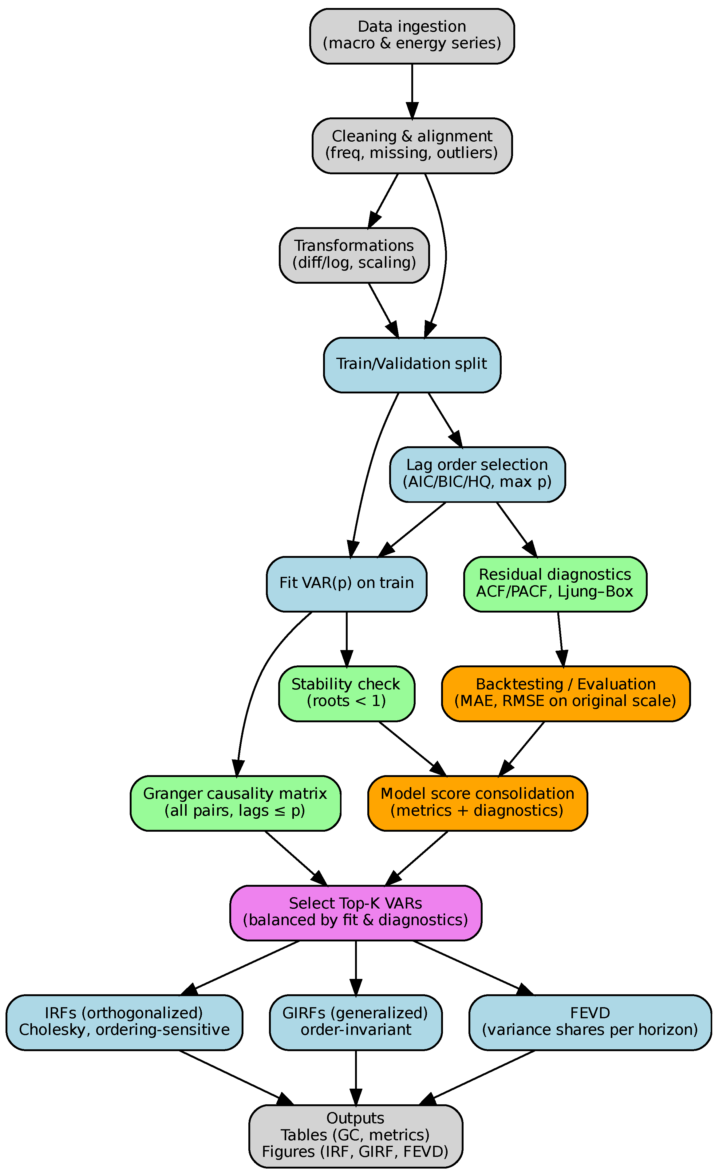
Figure 1 summarizes the methodological pipeline guiding this study. The workflow begins with the ingestion and harmonization of macroeconomic, energy, and environmental series, ensuring consistent frequency, treatment of missing observations, and screening for anomalies. Appropriate transformations (differencing, logarithmic scaling, standardization) are applied according to the stochastic properties of each variable.
A train–validation split maintains temporal integrity, after which optimal lag length is selected using AIC, BIC, and HQ criteria under a maximum-lag constraint. The VAR(p) is then estimated on the training sample and subjected to standard diagnostics—including residual autocorrelation tests, Ljung–Box statistics, and stability analysis based on companion-matrix roots—to verify model adequacy.
Models passing these checks are evaluated through two complementary steps. First, backtesting on the validation sample reconstructs forecasts on the original scale to obtain interpretable error metrics (MAE, RMSE). Second, diagnostic indicators and information-criteria scores are consolidated to rank competing lag specifications, enabling the selection of the best-performing VARs.
For the selected models, Granger causality tests reveal directional linkages, while impulse response functions (IRFs), generalized IRFs (GIRFs), and forecast error variance decomposition (FEVD) quantify the magnitude, persistence, and relative importance of shocks within the coupled macro–energy–environment system. These instruments provide the foundation for the Results section, where dynamic responses are translated into economically meaningful insights about Mexico’s structural dependence on hydrocarbons and its transition constraints.
4. Results
4.1. Generalized Impulse Response Functions (GIRFs)
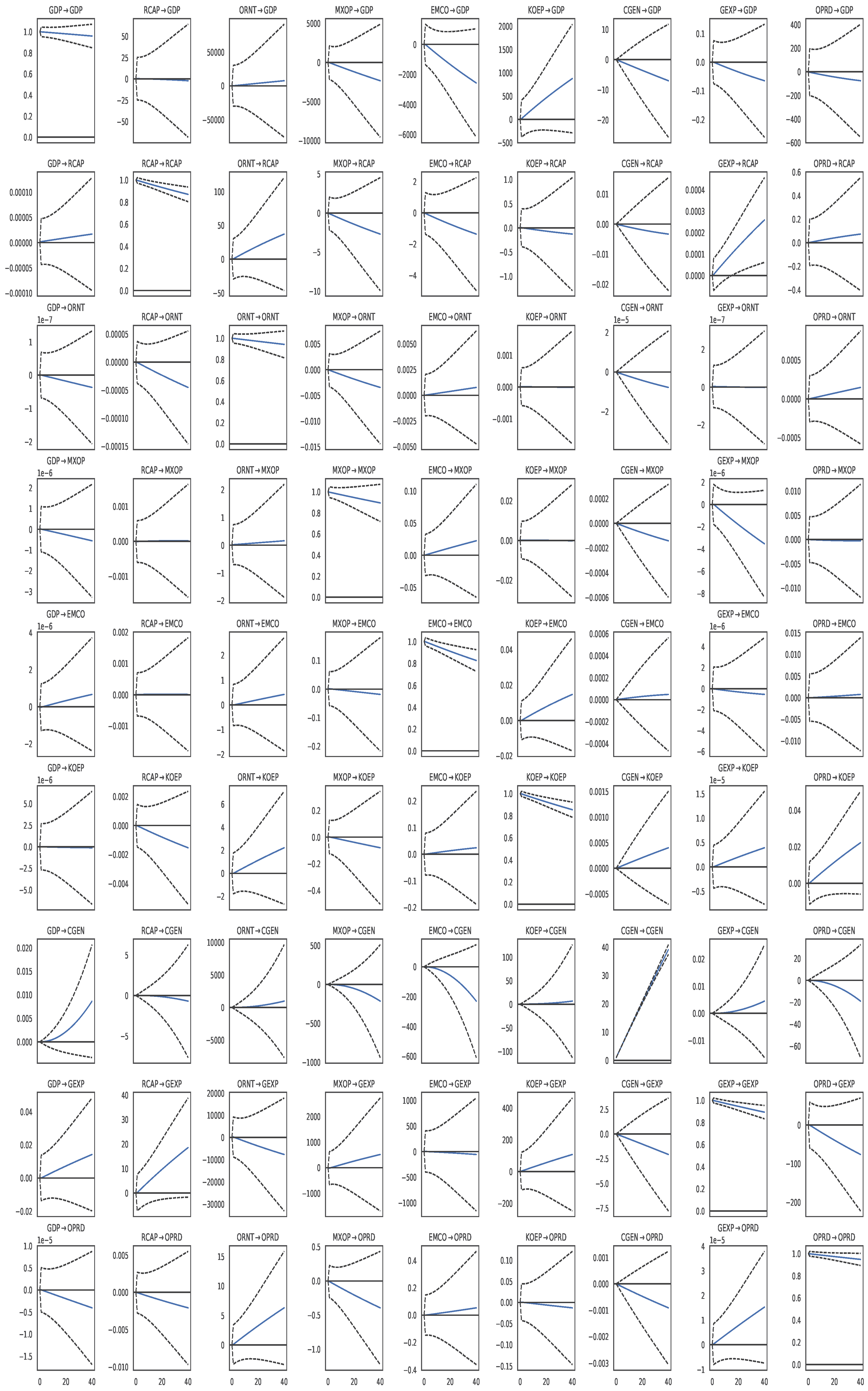
Generalized impulse response functions (GIRFs), which are invariant to variable ordering, are presented as the primary dynamic evidence from the estimated VAR model.
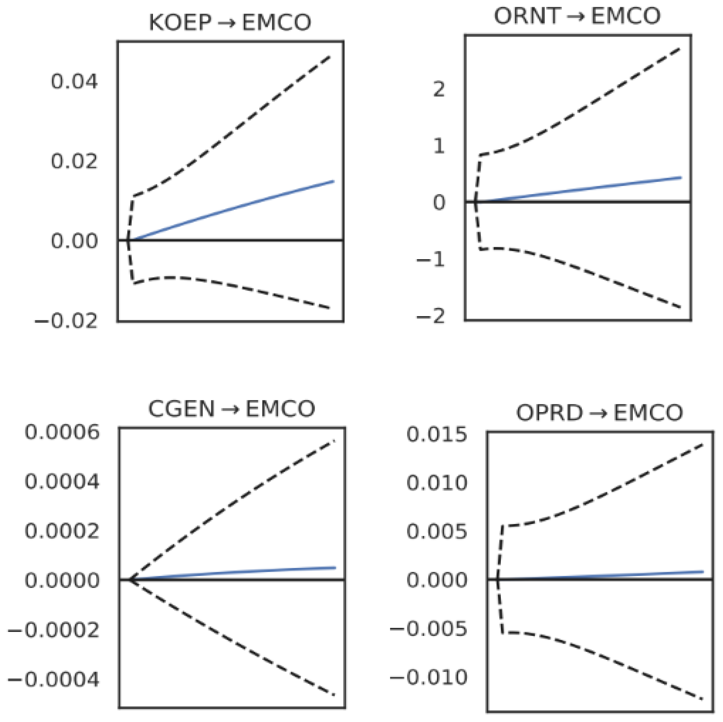
Figure 2 and
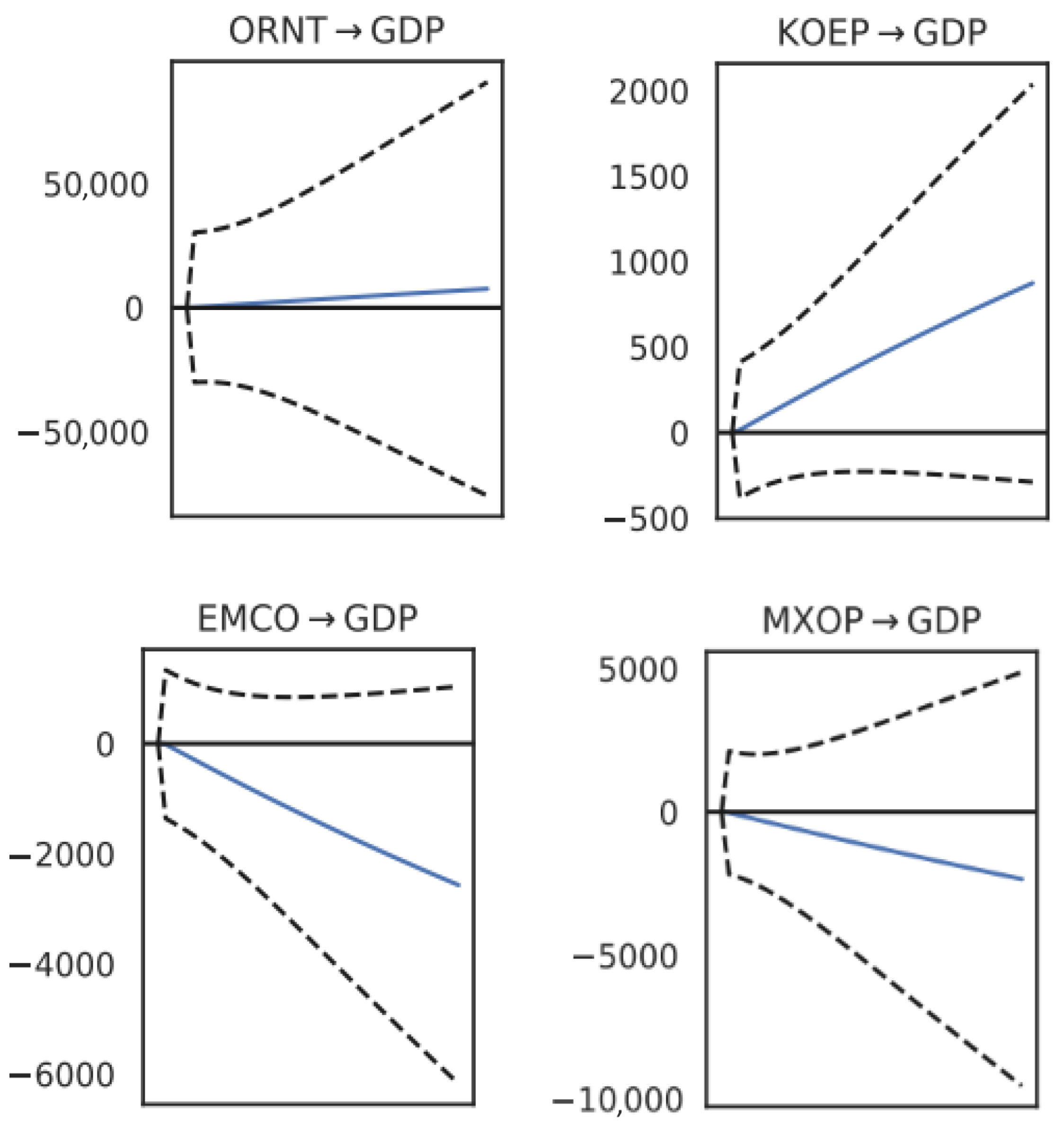
Figure 3 illustrate the GIRFs over a 40-day horizon. The results indicate that oil rents and energy consumption exert a positive and statistically significant impact on GDP, whereas shocks to coal-fired generation (CGEN) and oil prices (MXOP) have a negative effect on economic growth.
Renewable capacity (RCAP) expands in tandem with GDP but exerts only a marginal autonomous effect, reflecting its reliance on revenues generated from fossil fuels. CO2 emissions respond positively to shocks in oil rents, crude oil production, energy consumption, and fossil-based generation, underscoring the persistence of a carbon-intensive system. These patterns align with theoretical expectations and emphasize the asymmetric role of hydrocarbons as systemic drivers, with electricity generation and emissions functioning primarily as outcomes.
Finally, the Mexican crude oil price emerges as a key determinant of GDP dynamics. If PEMEX fails to reduce operational costs, an increase in the export blend price transmits negatively to GDP, weakening the economy’s growth cycle: savings → investment → capital accumulation rates → production → wages → economic growth (GDP). The complete set of impulse–response results is provided in
Appendix A and
Appendix B.
4.2. Impulse Response Functions (IRFs): Validation
Orthogonal impulse response functions (IRFs), estimated through a Cholesky decomposition, are computed to provide a benchmark for comparison with the generalized IRFs (GIRFs). Although orthogonal IRFs are sensitive to variable ordering, the results broadly corroborate the GIRF evidence: GDP responds positively to oil rents and energy consumption, but negatively to coal-fired generation and oil price shocks. Similarly, CO
2 emissions rise following fossil-related shocks. The convergence between GIRFs and orthogonal IRFs reinforces the robustness of the findings, as summarized in
Table 1, which reports the sign and magnitude of key responses at horizon
.
4.3. Forecast Error Variance Decomposition (FEVD)
The forecast error variance decomposition (FEVD) (
Kilian & Lütkepohl, 2017) assesses the relative importance of each variable in explaining the prediction errors of others, distinguishing between short- and medium-term effects. The results reveal heterogeneous patterns of interdependence within Mexico’s energy–economy system.
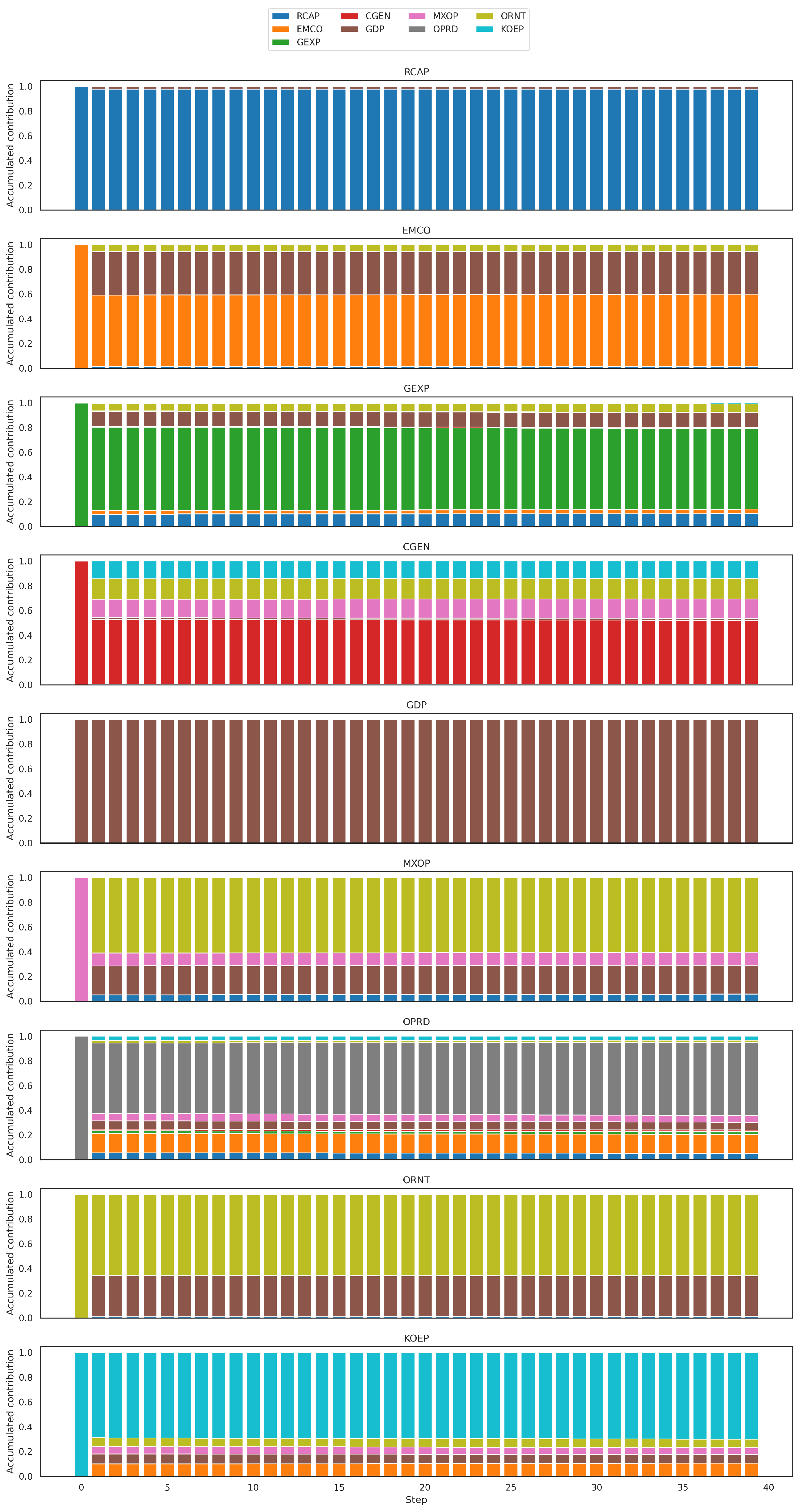
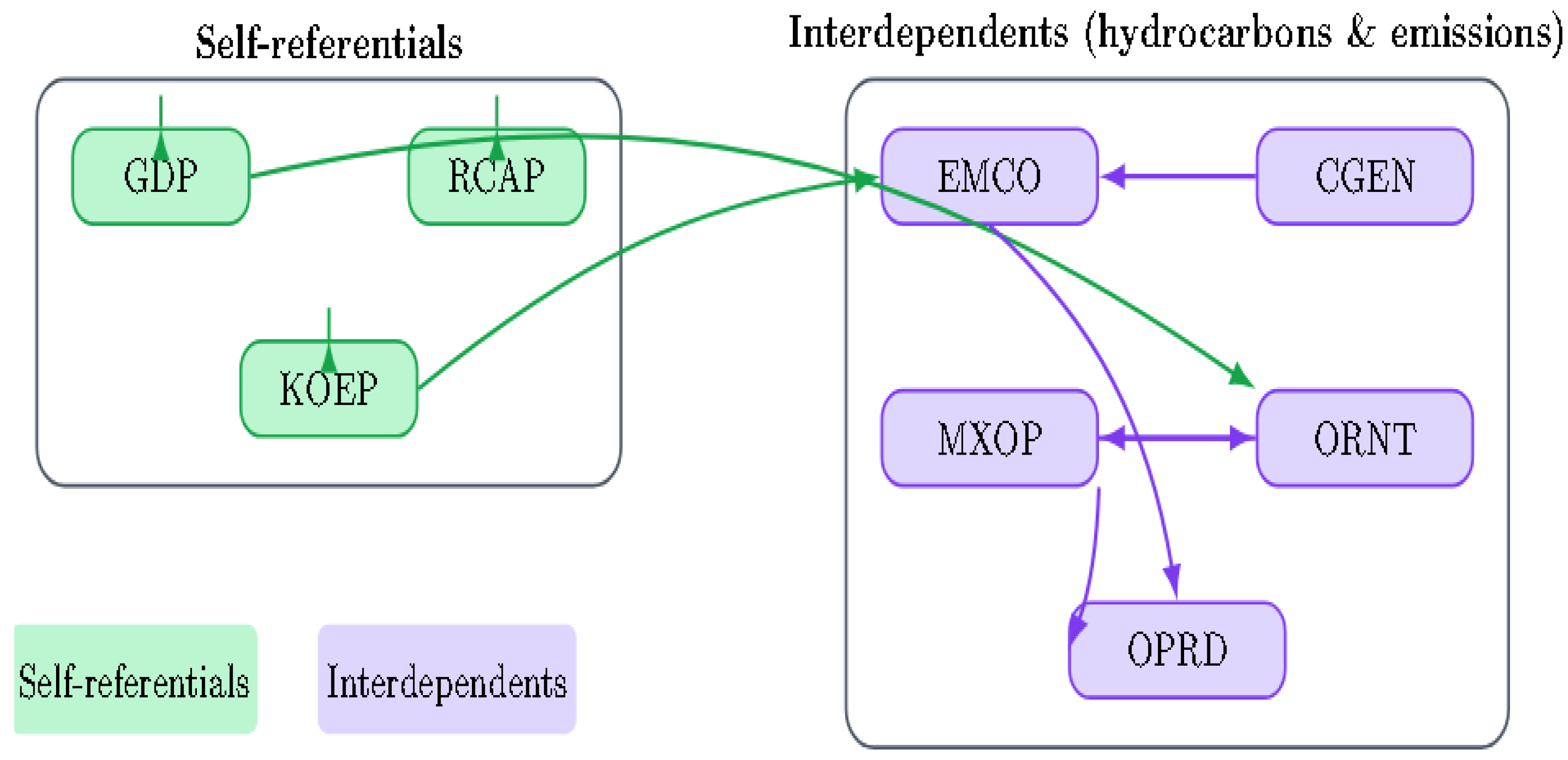
GDP exhibits a variance explained almost entirely by its own shocks, reflecting strong inertia and the self-referential nature of its macroeconomic dynamics throughout the model horizon. Similarly, renewable energy capacity (RCAP) and energy consumption (KOEP) are predominantly driven by their own shocks, indicating limited impulse transmission to or from the rest of the system.
By contrast, CO2 emissions display a high proportion of variance explained by shocks to energy consumption and coal-fired generation (CGEN), consistent with Mexico’s energy matrix remaining heavily fossil-based. Public expenditure (GEXP), although self-driven in the short term, becomes increasingly influenced by GDP and oil rents at medium horizons, underscoring the dependence of fiscal stability on energy-related revenues.
Coal-fired generation evolves from being primarily explained by its own shocks in the short term to being increasingly influenced by emissions and energy consumption in the long run, reflecting its intermediate role in the energy–environment transmission channel. Crude oil production (OPRD), while largely self-driven in the short term, shows long-run contributions from oil prices (MXOP) and emissions, highlighting the interplay between market dynamics, production, and environmental outcomes.
The Mexican oil price (MXOP) and oil rents (ORNT) display more balanced interactions; oil rents combine their own shocks with influences from GDP and oil prices, reflecting their role as a bridge between the real economy and hydrocarbon dynamics. Oil prices, in turn, are not explained solely by their own shocks but also reflect feedback from production and oil rents, consistent with the structurally integrated nature of the sector.
Overall, the FEVD confirms that while certain variables (GDP, renewable capacity, and energy consumption) follow strongly self-referential dynamics, others (CO
2 emissions, coal-fired generation, oil prices, crude oil production, and oil rents) exhibit significant interdependence (see
Figure 4). These results underscore the persistence of fossil fuel dependence and the need for renewable capacity to evolve toward deeper integration with Mexico’s national energy and economic system. The complete set of FEVD charts is provided in
Appendix C.
4.4. Granger Causality and Robustness Checks
Pairwise Granger causality tests provide additional evidence on directional relationships (
Granger, 1969). The results confirm that coal-fired generation functions primarily as a systemic receptor, dependent on virtually all other variables, while emissions predominantly reflect shocks from hydrocarbons, energy consumption, and fiscal expenditure. Additional linkages of interest include the direct relationship of coal-fired generation → CO
2 and the weak feedback of coal-fired generation → renewables, suggesting that fossil infrastructure constrains renewable expansion trajectories. Moreover, the fiscal–energy transmission channel is evident in the relationship of public expenditure → oil price, underscoring the role of fiscal policy as a propagation mechanism within the oil cycle.
Robustness checks using generalized IRFs (GIRFs) confirm that the main patterns hold, regardless of variable ordering. In both orthogonal IRFs and GIRFs, oil rents, energy consumption, and hydrocarbon production exert a positive and statistically significant effect on GDP, while coal-fired generation and oil price shocks negatively affect economic growth. Similarly, the positive association between oil rents and CO
2 emissions, as well as the role of energy consumption in increasing carbon intensity, remain consistent across methodologies. Minor differences in magnitude indicate some sensitivity to identification: the links between GDP and renewable capacity and between coal-fired generation and emissions appear weaker in GIRFs, while the impact of public expenditure on CO
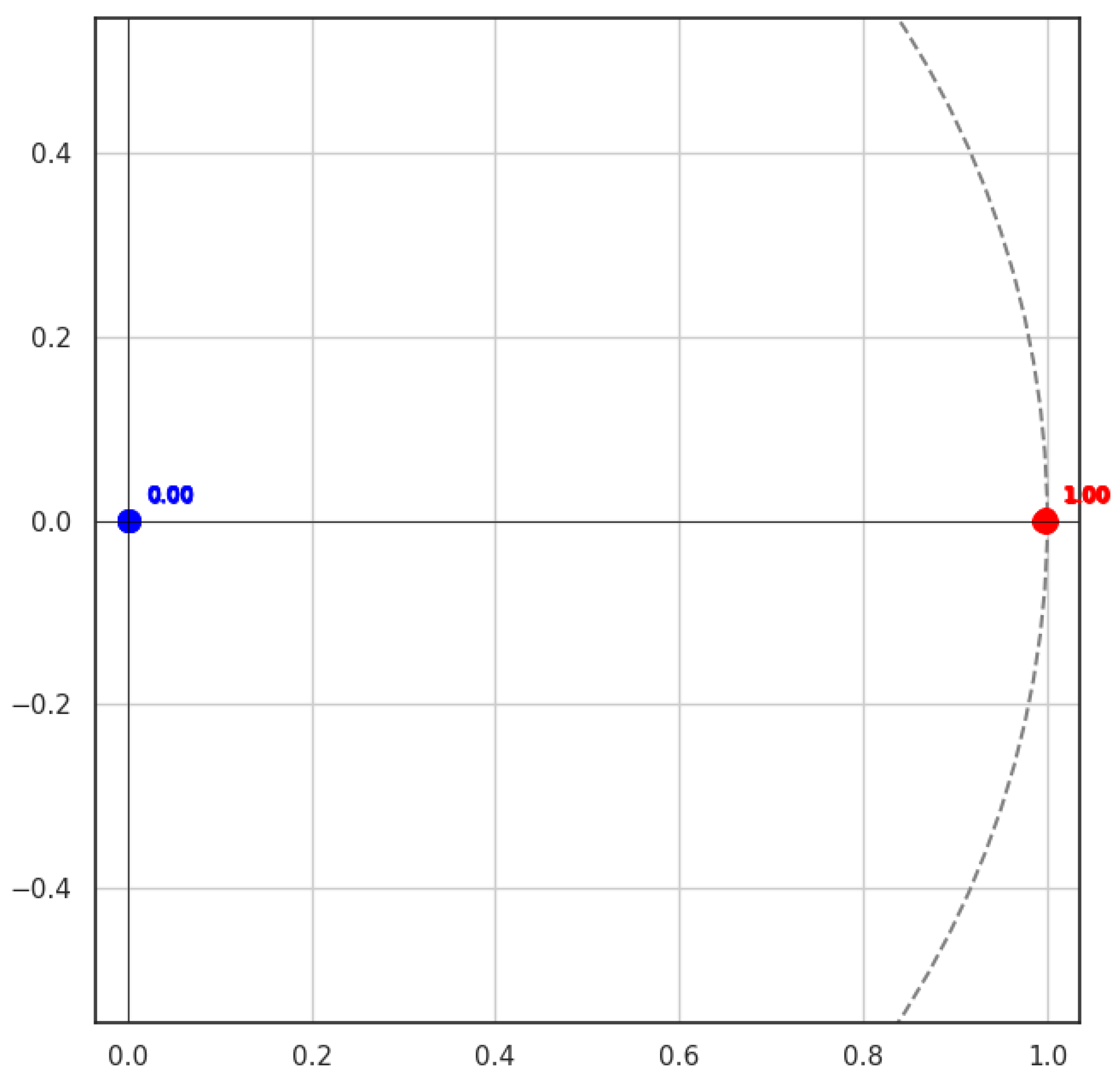
2 is attenuated. These variations do not alter the overall direction of the results but highlight the importance of combining IRFs with GIRFs to ensure robustness. Stability analysis further verifies that all eigenvalues lie within the unit circle, confirming the reliability of the VAR specification (see
Figure 5).
5. Discussion
The results of the VAR analysis—supported by impulse response functions (IRFs), forecast error variance decomposition (FEVD), Granger causality tests, and generalized IRFs (GIRFs)—confirm Mexico’s structural dependence on the hydrocarbon sector. Oil rents exert a persistent positive influence on GDP growth, while renewable energy capacity has yet to generate an autonomous or significant contribution to economic performance. The vulnerability of GDP to oil price shocks further underscores the need for PEMEX to modernize its cost structure and improve operational efficiency.
Granger causality tests reinforce these findings: hydrocarbons and fiscal policy emerge as key predictive drivers, whereas coal-fired generation and CO2 emissions act predominantly as receivers of systemic shocks. GIRF analysis corroborates the main patterns identified through orthogonal IRFs, showing that oil rents, energy consumption, and hydrocarbon production contribute positively to GDP, while coal-fired generation and oil prices exert negative effects. Differences in magnitude across methods suggest sensitivity in certain relationships—such as GDP–renewables and coal–emissions—but the overall conclusions remain consistent. Collectively, these results highlight both the resilience and fragility of Mexico’s energy–economy system.
5.1. Comparison with Previous Studies
Our findings align with and extend earlier VAR-based studies of energy–economy linkages.
Kousar et al. (
2022) demonstrate how exchange rate dynamics and fiscal deficits amplify energy inflation, underscoring the role of macroeconomic structures. Similarly,
Orzechowski and Bombol (
2022) show that financial instruments such as green bonds are critical for sustaining energy security. Focusing on Azerbaijan,
Mukhtarov et al. (
2021) report that oil price shocks are central determinants of macroeconomic performance, shaping both exchange rates and external balances.
In comparison, the Mexican experience reveals a distinct pattern: oil rents function not only as a source of vulnerability but also as the main enabler of fiscal and energy investments. The IRF, FEVD, and Granger evidence suggests that although renewable capacity is positively linked to growth, its reliance on oil-derived revenues creates a feedback loop that delays Mexico’s decoupling from hydrocarbons. Generalized impulse response functions, as proposed by
Pesaran and Shin (
1998), confirm the robustness of these findings, adding confidence that they are not artifacts of variable ordering. This underscores a dual challenge: sustaining fiscal stability while advancing an effective energy transition.
5.2. Implications for Mexico’s Energy Policy
The FEVD results show that CO2 emissions, crude oil production, and public expenditure remain tightly intertwined with oil revenues and prices. This indicates that fiscal stability and environmental outcomes continue to depend on PEMEX’s performance. For policymakers, the findings highlight the urgency of diversifying public revenues away from oil rents and fostering an institutional framework that attracts private renewable investment. Without such reforms, the renewable sector will remain indirectly financed by hydrocarbon cycles, limiting its ability to deliver sustained economic returns and emissions reductions.
Granger causality and GIRF results provide further insights. Public expenditure emerges as a non-negligible driver, influencing both oil prices and coal-fired generation, thereby revealing the fiscal–energy transmission channel. The dependence of coal-fired generation on nearly all other variables underscores its dual vulnerability: it absorbs but does not generate systemic impulses, while imposing economic and environmental costs. Transitioning away from coal-based capacity toward renewable sources such as solar photovoltaics, onshore wind, or geothermal—areas where Mexico holds clear comparative advantages—appears essential. Although politically and economically challenging, such a transition aligns with long-term growth and climate commitments. Modernizing PEMEX and strengthening the renewable framework should therefore be seen as complementary rather than competing priorities.
5.3. Limitations and Future Research
This study has several limitations. First, the reduced-form VAR framework captures linear short- and medium-run dependencies but does not model potential nonlinearities or structural breaks in Mexico’s energy history. Extensions using structural, nonlinear, or time-varying parameter VARs could provide a richer characterization of the transmission mechanisms identified here (
Lütkepohl, 2005).
Second, the empirical design is explicitly macroeconomic, focusing on aggregate interactions among output, fiscal revenues, energy use, and emissions. As such, the analysis does not incorporate the technological or plant-level detail commonly required in micro-scale assessments of energy systems. Moving from macro to micro perspectives—such as evaluating technology-specific costs, environmental impacts, or the competitiveness of particular generation options—represents a natural extension of this line of research. Future work could therefore use the macro-level insights obtained here as a basis for more detailed techno-economic studies that examine how structural energy–economy dynamics translate into operational or project-level decisions.
Finally, hybrid econometric–machine learning approaches, including ARIMA–LSTM or GARCH–LSTM architectures, offer promising avenues for capturing nonlinear or regime-dependent dynamics and improving forecasting performance. Ongoing work by the authors will explore these hybrid frameworks in the context of Mexico’s energy and fiscal systems.
6. Conclusions
This study employed a reduced-form VAR framework to quantify the short- and medium-run dynamic interactions between Mexico’s energy, fiscal, and environmental subsystems under conditions of limited information. Across IRFs, GIRFs, FEVD, and Granger causality, a consistent and robust pattern emerges: hydrocarbons function as the central transmission mechanism linking economic activity, public finances, and emissions. Oil rents exert a persistent positive influence on GDP and government expenditure, while crude oil prices and coal-fired generation impose negative shocks to output and raise carbon intensity. These dynamics depict a structurally constrained energy–economy system in which hydrocarbon dependence remains a dominant source of both stimulus and vulnerability.
Renewable capacity behaves pro-cyclically and exhibits limited autonomous effects, indicating that its expansion continues to rely indirectly on resources, revenues, and momentum generated by fossil activities. This suggests that Mexico’s renewable sector is not yet macroeconomically integrated: it follows the business cycle but does not shape it. In parallel, CO2 emissions respond strongly to shocks in energy consumption, oil rents, and coal-fired generation, reaffirming that environmental outcomes remain tightly coupled to the fossil subsystem.
The FEVD results reinforce this interpretation. GDP, renewable capacity, and energy use are primarily self-driven, whereas oil production, oil prices, and emissions exhibit strong mutual dependencies. This asymmetry indicates that Mexico’s macroeconomic stability is influenced disproportionately by hydrocarbon dynamics, while emerging low-carbon technologies have not yet reached a scale capable of generating independent macroeconomic impulses.
Taken together, these findings portray a system in which short- and medium-run economic resilience continues to hinge on PEMEX’s operational performance and the volatility of global oil markets. Strengthening PEMEX’s efficiency, diversifying fiscal revenues, and improving institutional conditions for renewable investment emerge not as competing objectives, but as jointly necessary steps to reduce systemic vulnerability. The evidence suggests that without progress on these fronts, Mexico’s transition will remain fiscally dependent on hydrocarbons and environmentally not aligned with global decarbonization trajectories.
Finally, the study demonstrates that even under limited and mixed-frequency data—a common constraint in emerging economies—a transparent VAR-based framework can reveal the propagation structure of energy–economy interactions. This provides a reproducible empirical basis for evaluating transition pathways and offers a methodological template that can be extended in future research using structural, nonlinear, or time-varying parameter models applicable to other resource-dependent economies.
Author Contributions
Conceptualization, J.A.M.-H. and M.D.l.P.-R.; Methodology, J.A.M.-H., R.C.M.-H., and M.D.l.P.-R.; Software, J.A.M.-H.; Validation, R.C.M.-H. and M.D.l.P.-R.; Formal analysis, J.A.M.-H. and R.C.M.-H.; Investigation, J.A.M.-H. and M.D.l.P.-R.; Resources, J.A.J.-B., D.S., C.d.C.G.-T., and J.G.B.-S.; Data curation, M.D.l.P.-R.; Writing—original draft preparation, J.A.M.-H., R.C.M.-H., and M.D.l.P.-R.; Writing—review and editing, J.A.M.-H., R.C.M.-H., J.A.J.-B., D.S., C.d.C.G.-T., and J.G.B.-S.; Visualization, J.A.M.-H. and R.C.M.-H.; Supervision, J.A.J.-B., D.S., C.d.C.G.-T., and J.G.B.-S.; Project administration, J.A.J.-B., D.S., C.d.C.G.-T., and J.G.B.-S.; Funding acquisition, J.A.J.-B., D.S., C.d.C.G.-T., and J.G.B.-S. All authors have read and agreed to the published version of the manuscript.
Funding
This research received no external funding.
Institutional Review Board Statement
Not applicable.
Informed Consent Statement
Not applicable.
Data Availability Statement
The study relies on publicly available datasets obtained from the Banco de México, INEGI, CEFP, World Bank (WDI), SENER/SIE, and PEMEX. All data sources are fully documented within the replication files. Replication code and datasets used in this analysis are openly accessible at
https://github.com/Adri0103-coding-mx/Mexico-Energy-Economy-VAR (accessed on 11 November 2025), ensuring the transparency and reproducibility of all empirical results.
Acknowledgments
The authors thank the Instituto Politécnico Nacional (IPN) for academic support, particularly the Escuela Superior de Ingeniería Mecánica y Eléctrica (ESIME), Unidad Zacatenco, as the doctoral program’s home institution. We also acknowledge the Centro de Investigación en Computación (CIC) and the Escuela Superior de Economía (ESE) of the Instituto Politécnico Nacional for their contributions in computational and economic training, respectively. Additional thanks are extended to colleagues from IPICYT for their valuable feedback throughout this study. Constructive discussions within our institutional collaboration significantly improved the clarity and scope of the manuscript.
Conflicts of Interest
The authors declare no conflicts of interest.
Abbreviations
The following abbreviations are used in this manuscript:
| VAR | Vector Autoregression |
| IRF | Impulse Response Function |
| GIRF | Generalized Impulse Response Function |
| FEVD | Forecast Error Variance Decomposition |
| ADF | Augmented Dickey–Fuller (test) |
| PP | Phillips–Perron (test) |
| KPSS | Kwiatkowski–Phillips–Schmidt–Shin (test) |
| AIC | Akaike Information Criterion |
| BIC | Bayesian Information Criterion |
| HQIC | Hannan–Quinn Information Criterion |
| PEMEX | Petróleos Mexicanos |
| GDP | Gross Domestic Product at current prices |
| RCAP | Renewable installed capacity (MW) |
| ORNT | Oil rents (% of GDP) |
| EMCO | CO2 emissions (Mt) |
| KOEP | Energy Use (kg of oil equivalent per capita) |
| CGEN | Coal-fired gross electricity Generation (GWh) |
| GEXP | Government Expenditure |
| OPRD | Crude Oil Production (kb/d) |
| MXOP | Mexican Blend crude oil price (USD) |
Appendix A
Full generalized impulse–response chart.
Figure A1.
Generalized impulses–responses (GIRFs). Note: Solid lines represent the point estimates of the generalized impulse–response functions. Dashed lines denote the 95% bootstrap confidence intervals, and the horizontal zero line marks the no–effect baseline.
Figure A1.
Generalized impulses–responses (GIRFs). Note: Solid lines represent the point estimates of the generalized impulse–response functions. Dashed lines denote the 95% bootstrap confidence intervals, and the horizontal zero line marks the no–effect baseline.
Appendix B
Full impulse–response chart.
Figure A2.
Impulses–responses (IRFs). Note: Solid lines represent the point estimates of the impulse–response functions (IRFs). Dashed lines denote the 95% bootstrap confidence intervals, and the horizontal zero line marks the no–effect baseline.
Figure A2.
Impulses–responses (IRFs). Note: Solid lines represent the point estimates of the impulse–response functions (IRFs). Dashed lines denote the 95% bootstrap confidence intervals, and the horizontal zero line marks the no–effect baseline.
Appendix C
Full forecast error variance decomposition chart.
Figure A3.
Forecast error variance decomposition (FEVD). Each color corresponds to one of the VAR shocks: RCAP, EMCO, GEXP, CGEN, GDP, MXOP, OPRD, ORNT, and KOEP. The stacked bars show how the contribution of each shock to the forecast error variance evolves across horizons.
Figure A3.
Forecast error variance decomposition (FEVD). Each color corresponds to one of the VAR shocks: RCAP, EMCO, GEXP, CGEN, GDP, MXOP, OPRD, ORNT, and KOEP. The stacked bars show how the contribution of each shock to the forecast error variance evolves across horizons.
References
- Acheampong, A. O. (2018). Economic growth, CO2 emissions and energy consumption: What causes what and where? Energy Economics, 74, 677–692. [Google Scholar] [CrossRef]
- Akaike, H. (1974). A new look at the statistical model identification. IEEE Transactions on Automatic Control, 19, 716–723. [Google Scholar] [CrossRef]
- Banco de México (Banxico). (2025). Statistics and indicators. Available online: https://www.banxico.org.mx (accessed on 24 September 2025).
- Baumeister, C., & Peersman, G. (2013). Time-varying effects of oil supply shocks on the US economy. American Economic Journal: Macroeconomics, 5, 1–28. [Google Scholar] [CrossRef]
- Blanchard, O. J., & Quah, D. (1989). The dynamic effects of aggregate demand and supply disturbances. American Economic Review, 79, 655–673. [Google Scholar]
- BP. (2023). Statistical review of world energy 2023. Energy Institute. Available online: https://www.energyinst.org/statistical-review (accessed on 5 January 2025).
- Dickey, D. A., & Fuller, W. A. (1979). Distribution of the estimators for autoregressive time series with a unit root. Journal of the American Statistical Association, 74, 427–431. [Google Scholar] [CrossRef]
- El Anshasy, A. A., & Bradley, M. D. (2012). Oil prices and the fiscal policy response in oil-exporting countries. Journal of Policy Modeling, 34, 605–620. [Google Scholar] [CrossRef]
- Engle, R. F., & Granger, C. W. J. (1987). Cointegration and error correction: Representation, estimation, and testing. Econometrica, 55, 251–276. [Google Scholar] [CrossRef]
- Farzanegan, M. R., & Markwardt, G. (2009). The effects of oil price shocks on the Iranian economy. Energy Economics, 31, 134–151. [Google Scholar] [CrossRef]
- Granger, C. W. J. (1969). Investigating causal relations by econometric models and cross-spectral methods. Econometrica, 37, 424–438. [Google Scholar] [CrossRef]
- Hamilton, J. D. (1983). Oil and the macroeconomy since World War II. Journal of Political Economy, 91, 228–248. [Google Scholar] [CrossRef]
- Hannan, E. J., & Quinn, B. G. (1979). The determination of the order of an autoregression. Journal of the Royal Statistical Society Series B, 41(2), 190–195. [Google Scholar] [CrossRef]
- IEA. (2023). Global energy review 2023. International Energy Agency. Available online: https://www.iea.org/reports/global-energy-review-2023 (accessed on 5 January 2025).
- Instituto Nacional de Estadística y Geografía (INEGI). (2025). Banco de información económica. Available online: https://www.inegi.org.mx (accessed on 24 September 2025).
- International Energy Agency (IEA). (2025). IEA data and statistics. Available online: https://www.iea.org/data-and-statistics (accessed on 24 September 2025).
- International Monetary Fund (IMF). (2024). Mexico: 2024 article IV consultation (IMF Country Report No. 2024/317). Available online: https://www.imf.org/en/Publications/CR/Issues/2024/11/01/Mexico-2024-Article-IV-Consultation-and-Review-Under-the-Flexible-Credit-Line-Arrangement-556997 (accessed on 11 November 2025).
- Johansen, S. (1991). Estimation and hypothesis testing of cointegration vectors in Gaussian vector autoregressive models. Econometrica, 59, 1551–1580. [Google Scholar] [CrossRef]
- Kilian, L. (2009). Not all oil price shocks are alike: Disentangling demand and supply shocks in the crude oil market. The American Economic Review, 99, 1053–1069. [Google Scholar] [CrossRef]
- Kilian, L., & Lütkepohl, H. (2017). Structural vector autoregressive analysis. Cambridge University Press. [Google Scholar] [CrossRef]
- Koengkan, M., Fuinhas, J. A., & Rosa, S. B. (2021). The energy-economic growth nexus in Latin American and the Caribbean countries: A new approach with globalisation index. Revista Valore, 5, e-5019. [Google Scholar] [CrossRef]
- Koop, G., Pesaran, M. H., & Potter, S. M. (1996). Impulse resrponse analysis in nonlinear multivariate models. Journal of Economics, 74, 119–147. [Google Scholar] [CrossRef]
- Kousar, S., Sabir, S. A., Ahmed, F., & Bojnec, Š. (2022). Climate change, exchange rate, twin deficit, and energy inflation: Application of VAR model. Energies, 15(20), 7663. [Google Scholar] [CrossRef]
- Kwiatkowski, D., Phillips, P. C. B., Schmidt, P., & Shin, Y. (1992). Testing the null hypothesis of stationarity against the alternative of a unit root. Journal of Economics, 54, 159–178. [Google Scholar] [CrossRef]
- Lütkepohl, H. (2005). New introduction to multiple time series analysis. Springer. [Google Scholar] [CrossRef]
- Marín-Rodríguez, J., Pereira, J., & Gómez, F. (2025). Economic policy uncertainty and energy shocks in Latin America: A TVP-VAR analysis. Applied Economics. in press. [Google Scholar]
- Mukhtarov, S., Yüksel, S., & Mammadov, J. (2021). The impact of oil price shocks on national income: Evidence from Azerbaijan. Energies, 14(6), 1695. [Google Scholar] [CrossRef]
- Natural Resource Governance Institute (NRGI). (2025). Pemex and the energy transition: Timely responses to growing threats. Available online: https://resourcegovernance.org/publications/pemex-and-energy-transition-timely-responses-growing-threats (accessed on 11 November 2025).
- Nepal, R., & Paija, N. (2019). A multivariate time series analysis of energy consumption, real output and pollutant emissions in a developing economy: New evidence from Nepal. Economic Modelling, 77, 164–173. [Google Scholar] [CrossRef]
- OECD. (2024). OECD economic surveys: Mexico 2024. OECD Publishing. [Google Scholar] [CrossRef]
- Orzechowski, R., & Bombol, M. (2022). Energy security, sustainable development and the green bond market. Energies, 15(17), 6218. [Google Scholar] [CrossRef]
- PEMEX. (2025). Anuario estadístico y reportes operativos/financieros. Available online: https://www.pemex.com (accessed on 24 September 2025).
- Pesaran, M. H., & Shin, Y. (1998). Generalized impulse response analysis in linear multivariate models. Economics Letters, 58, 17–29. [Google Scholar] [CrossRef]
- Phillips, P. C. B., & Perron, P. (1988). Testing for a unit root in time series regression. Biometrika, 75, 335–346. [Google Scholar] [CrossRef]
- Ratti, R. A., & Vespignani, J. L. (2016). Oil prices and global factor macroeconomic variables. Energy Economics, 59, 198–212. [Google Scholar] [CrossRef]
- Schwarz, G. (1978). Estimating the dimension of a model. Annals of Statistics, 6, 461–464. [Google Scholar] [CrossRef]
- Secretaría de Energía (SENER). (2025). Sistema de Información Energética (SIE). Available online: https://sie.energia.gob.mx (accessed on 24 September 2025).
- Sims, C. A., Stock, J. H., & Watson, M. W. (1990). Inference in linear time series models with some unit roots. Econometrica, 58, 113–144. [Google Scholar] [CrossRef]
- Sovacool, B. K. (2016). How long will it take? Conceptualizing the temporal dynamics of energy transitions. Energy Research & Social Science, 13, 202–215. [Google Scholar] [CrossRef]
- Stock, J. H., & Watson, M. W. (2001). Vector autoregressions. Journal of Economic Perspectives, 15, 101–115. [Google Scholar] [CrossRef]
- Uhlig, H. (2005). What are the effects of monetary policy on output? Results from an agnostic identification procedure. Journal of Monetary Economics, 52, 381–419. [Google Scholar] [CrossRef]
- Van de Graaf, T., & Colgan, J. D. (2016). Global energy governance: A review and research agenda. Palgrave Communications, 2, 15047. [Google Scholar] [CrossRef]
- World Bank. (2025). World development indicators (WDI). Available online: https://databank.worldbank.org/source/world-development-indicators (accessed on 24 September 2025).
| Disclaimer/Publisher’s Note: The statements, opinions and data contained in all publications are solely those of the individual author(s) and contributor(s) and not of MDPI and/or the editor(s). MDPI and/or the editor(s) disclaim responsibility for any injury to people or property resulting from any ideas, methods, instructions or products referred to in the content. |
© 2025 by the authors. Licensee MDPI, Basel, Switzerland. This article is an open access article distributed under the terms and conditions of the Creative Commons Attribution (CC BY) license (https://creativecommons.org/licenses/by/4.0/).
