Abstract
This paper examines the relationship between economic growth and rural unemployment in Brazil and Mexico, incorporating the effects of climate variability and spatial interactions. Okun’s Law serves as the theoretical framework, and a dynamic spatial panel model is applied to estimate short-term causal effects. The analysis uses data from Brazil’s IBGE, Mexico’s INEGI, and the U.S. NCEI. The results indicate that Okun’s Law is only partially validated in Mexico, where lagged income growth reduces rural unemployment, while in Brazil, the relationship is not statistically confirmed. Climate variables also play a critical role: higher local temperatures reduce unemployment in Brazil and, with a lag, in Mexico, although temperature increases in neighboring regions raise unemployment in Mexico. Rainfall has a consistent positive effect on rural unemployment in both countries, highlighting the disruptive impact of extreme weather events. From a spatial perspective, no contemporaneous effects are observed. However, lagged spatial effects are negative in Brazil and positive in Mexico, suggesting different adjustment dynamics across territories. Overall, the findings reveal that climate variability influences the growth-unemployment nexus differently depending on the national context and temporal dimension. These results underscore the importance of designing public policies that integrate territorial coordination, address the differentiated impacts of climate variability, and strengthen the adaptive capacity and resilience of rural areas in Latin America.
1. Introduction
The environment is a central pillar for the social and economic development of rural areas, as well as for the sustainability of their ways of life. However, this relationship has become increasingly fragile due to the negative externalities of economic activities, including pollution, the overexploitation of natural resources, and biodiversity loss. These processes not only reduce environmental quality but also restrict development opportunities, erode income, and weaken long-term economic growth (Nakhle et al., 2024; Xu & Peng, 2024).
The degradation of rural ecosystems has dual consequences. On the environmental side, it accelerates climate variability and undermines biodiversity. On the economic side, it diminishes productive capacity, reduces resilience, and threatens the livelihoods of communities dependent on natural resources (Wei et al., 2024). These challenges highlight the limitations of a development model based on intensive resource exploitation and the need to rethink strategies for sustainability (Ajanaku & Collins, 2021; Gowdy & Salman, 2007).
Latin America and the Caribbean are especially exposed to these dynamics. The region has experienced significant deforestation and climate variability over recent decades, leading to biodiversity loss, reduced carbon capture, and pressure on rural economies (Armenteras et al., 2017). Although the region contributed only 8.3% of global greenhouse gas (GHG) emissions in 2014, it was disproportionately affected by climate impacts generated elsewhere (Comisión Económica para América Latina y el Caribe (CEPAL) & EUROCLIMA+, 2018). Agriculture, a key sector for rural livelihoods, is particularly vulnerable as climate change reduced regional agricultural productivity by 24.3% in 2015, far above the global average (15.9%). This drop translated into lower rural incomes, worsening inequality, and increased migration pressures.
Similarly, rural areas face more severe challenges in terms of climate change due to their geographical and socioeconomic characteristics. These include: (1) production that lacks technification and human capital training (Cardoso López & López Cabrera, 2023, 2025); (2) institutions without installed capacity to improve and diversify production (Estrada-Carmona et al., 2014); (3) the absence of total coverage in basic and quality education for work (Otero, 2019); (4) demographic changes, declining wages, and increases in migration (Jedwab et al., 2017); and (5) total dependence on the behavior of exogenous conditions associated with climate change and soil degradation (Mohaddes et al., 2023), among others. These limitations not only hinder economic diversification but also shape the functioning of rural labor markets, thereby heightening their exposure to climate-related risks.
Thus, from the conceptual framework of the Macroeconomics of Climate Change and Rural Development1, this study is based on the advances made by Cardoso López and López Cabrera (2023, 2025) and J. P. Elhorst and Emili (2022). The first and second extended the analysis of Okun’s Law to subnational scales, exploring its validity in the progressive transition from urban to rural contexts. Additionally, J. P. Elhorst and Emili (2022) incorporated an innovative approach by integrating spatial interdependencies in the estimation of this empirical relationship, demonstrating how local economic dynamics are intertwined with regional patterns.
This paper aims to estimate the empirical validity of Okun’s Law, through elasticities, incorporating the impact of climate variability on rural areas and from a short-term spatial and causal perspective. Accordingly, this paper addresses the following research question: To what extent does climate variability affect the empirical validity of Okun’s Law in the rural labor markets of Brazil and Mexico during the period 2012–2024?
The rationale for this question lies in the need to understand whether traditional macroeconomic relationships, such as Okun’s Law, remain valid under the structural constraints and vulnerabilities of rural areas, which are increasingly exposed to climate shocks. By focusing on subnational units and short-term spatial dynamics, this study explores how climate variability moderates the growth-employment nexus, providing highly relevant evidence for the design of rural development and labor market policies.
To this end, we use information from Mexico and Brazil, during the period 2012–2024, at the subnational level (Liu et al., 2025; Mohaddes et al., 2023). The choice of this period is justified by the availability of consistent and comparable information on both rural labor markets and climate conditions in these territories. To validate this relationship, a Spatial Durbin model with a Dynamic Panel is used, making it possible to capture both the spatial dependencies and the temporal dynamics of unemployment.
Analyzing these elasticities is key to understanding the sensitivity of rural unemployment to changes in income and to assessing more accurately the effectiveness of public policies in vulnerable environments and those exposed to climate risks. This methodological approach contributes to closing two critical gaps in the literature: (i) the scarcity of empirical evidence on Okun’s Law in interdependent rural economies, and (ii) the omission of climatic factors as moderating elements of this relationship.
The selection of these territories for analysis responds to their importance in the Latin American and the Caribbean region: Brazil and Mexico accounted for 57% of regional GDP in 2021 (CEPAL, 2020). Also, both countries have a high proportion of rural population (13.71% in Brazil and 20.13% in Mexico), vast agroecological and forestry extensions with respect to the total territory of the country (28.45% in Brazil and 49.82% in Mexico), and a significant contribution to the real agricultural value added of Latin America and the Caribbean (27.13% in Brazil and 13.16% in Mexico) in the period from 2012 to 2022, which makes them especially vulnerable to the effects of climate change (FAO et al., 2023). In addition, they are characterized by marked territorial inequalities, fragmented labor structures, and limited institutional capacity in their rural areas, which conditions employment and development dynamics (Dos Santos et al., 2024; Jessoe et al., 2018).
The results show that, although local real income growth does not always reduce unemployment due to structural rigidities, incomes in neighboring regions exert a mitigating effect on local rural unemployment consistent with Okun’s Law. Regarding climatic variables, differentiated effects are identified: in Brazil, higher temperatures favor economic diversification and reduce unemployment, while in Mexico, these variations increase labor vulnerability. In addition, extreme rainfall negatively impacts rural employment in both countries, with effects that spread spatially. These findings highlight the importance of considering the spatial and climate dimension in order to design effective policies that promote resilience and sustainable development in rural areas.
This paper is structured as follows: Section 2 offers a review of the literature on the relationship between economic growth and the labor market in the context of climate change in Latin America and the Caribbean. Section 3 develops the conceptual framework and explains how climate variability can influence rural unemployment. Section 4 describes the econometric methodology, while Section 5 presents the data and descriptive statistics used. Finally, the Results, Discussion and Conclusions are presented in Section 6, Section 7 and Section 8, respectively.
2. Literature Review
Many studies agreed that climate change has had negative effects on global economic growth, with particularly severe impacts in tropical regions and developing countries, such as those in Latin America and the Caribbean. For example, it was estimated that increases in global temperature could lead to significant reductions in the Gross Domestic Product (GDP) of low- and middle-income countries, due to adverse effects on productivity, health, and physical capital (Burke et al., 2015). These impacts not only reduced the rate of economic growth but also tended to amplify inequalities between regions (Islam & Winkel, 2017).
These effects on economic growth had important implications for the labor market, one of the most direct channels through which climate change affected population well-being. For example, the agricultural sector, which in several Latin American countries still represented an important source of informal and subsistence employment, was particularly vulnerable. Changes in rainfall patterns, the increased frequency of extreme events, and rising climate variability negatively affected rural income yields and stability (Thornton et al., 2014), which could lead to internal migrations and pressure on urban labor markets (Islam & Winkel, 2017; Leichenko & Silva, 2014).
In urban areas, climate change generated substantial economic impacts, aggravating pre-existing inequalities. One of the most relevant effects was the heat-induced loss of work productivity. Dell et al. (2012) estimated that, by 2050, urban heat stress could lead to a loss of labor equivalent to more than 0.2% of the GDP in China, disproportionately affecting low-wage sectors and thus contributing to income inequality.
At the regional level, the impacts of high temperatures were not homogeneous: low-income regions faced economic losses up to seven times larger than those in higher-income regions. This was also reflected in the effects of high temperatures on wages, which could increase in heat-sensitive occupations, while other labor groups experienced significant reductions in their income (Zhao et al., 2024). Along with the differentiated effects by region and income, some economic sectors, such as tourism, displayed a high vulnerability to climate change. In particular, countries where tourism accounted for a high proportion of the GDP were threatened in terms of the economic sustainability of the sector and its ability to contribute to the Sustainable Development Goals (Gasper et al., 2011; Scott et al., 2019).
In addition, other findings showed that climate change disproportionately affected the most vulnerable groups, particularly in developing countries, where the limited capacity to adapt to and mitigate the effects of climate change amplified its impact on income distribution and reinforced their dependence on agriculture, exposing them to inadequate adaptation strategies that could aggravate their situation (Arenas-Wong et al., 2023; Gasper et al., 2011; Mondal et al., 2023).
Moreover, according to Galbraith (2021), workers in sectors such as agriculture and construction faced increasing risks to their health and safety due to extreme heat, pollution, and the spread of infectious diseases. The latter, such as dengue or malaria, were transmitted through vectors (for example, mosquitoes) whose range and presence increased with climate change. These threats were particularly acute in the global south, where much of the work took place outdoors and labor protection conditions were often limited.
In addition to its effects on employment and income, climate change also compromised the physical pillars that sustained economic development, such as energy infrastructure, which was key to the continuity of economic activities and job creation. In Latin America and the Caribbean, where about 45% of electricity came from hydroelectric sources, the risks arising from climate change, such as alterations in rainfall patterns, rising temperatures, and the increased frequency of extreme events, seriously compromised the sustainability and operational capacity of the energy system. This energy vulnerability not only threatened supply security, but also had a negative impact on energy-intensive productive sectors, affecting economic growth and employment stability (Comisión Económica para América Latina y el Caribe (CEPAL) & EUROCLIMA+, 2018).
In the face of these challenges, organizations such as FAO (2018) and (Comisión Económica para América Latina y el Caribe (CEPAL) and EUROCLIMA+, 2018) stressed the need to articulate integrated responses that combined adaptation and mitigation. The transition to more sustainable and resilient economies in the region required investments in renewable energy, energy efficiency, green infrastructure, and training for green jobs. This process not only sought to reduce the environmental impact but also to transform the productive structure, generate employment, and promote social inclusion. To this end, long-term strategic planning that took advantage of climate action as a driver of innovation, productivity, and reduction in inequalities was key.
3. Theoretical Framework
This section develops the theoretical framework of the relationship between economic growth and the unemployment rate (also known as Okun’s Law), taking into account the effects of climate variability. To this end, the original formulation based on gaps—between unemployment and potential output—is analyzed, and then its version expressed in differences, in order to capture short-term dynamics that are more sensitive to exogenous variations (Cardoso López & López Cabrera, 2023, 2025; Okun, 1962; Pizzo, 2019).
We consider an initial version of Okun’s Law in gaps, which specifies that the cyclical component of unemployment is inversely related to the component of the logarithm of income or production, being:
Such that, there is an inverse relationship if . Additionally, it is necessary to establish the values of the potential production of unemployment () and income or production (). In this way, the differences between current and natural levels reflect market asymmetries (Pizzo, 2019). It is also worth noting that the component includes all the dynamics that are not observable within the production levels. In Equation (1), means the rural area in state in the reference country (Brazil or Mexico) in time . In addition, an indirect relationship is proposed aimed at assessing the effects of climate variability, through an extension of the function that incorporates these dimensions.
So, if this confirms that Okun’s Law is effective in rural areas (Cardoso López & López Cabrera, 2023, 2025). Finally, f climate variables (temperature and rainfall), are included in analyses to capture the indirect effects of climate variability on unemployment, under the hypothesis that alterations in these conditions can modify both the productive structure and the stability of rural employment (Mohaddes et al., 2023; Sathler et al., 2018).
The original specification adopted here is the gap-based version of Okun’s Law, widely recognized for its ability to capture the long-run relationship between potential output and the natural rate of unemployment. However, given the theoretical development and the empirical approach adopted, we incorporate the formula in differences, which allows us to approximate the short-term dynamics more precisely. This version does not imply estimating growth rates in the strict sense, but is used to calculate elasticities between changes in unemployment and output.
Expressing Okun’s Law in terms of growth rates makes it possible to identify more clearly the discrepancies between observed growth and potential output growth, and how these differences affect the evolution of unemployment (Pizzo, 2019). Pizzo (2019) assumes that this reformulation is especially useful in contexts where estimates of potential output are uncertain or where economic shocks are frequent, such as in rural areas exposed to exogenous variations, including those related to climate variability. In this sense, Equation (2) acquires the structure:
Under a constant potential growth rate, changes in unemployment are related to output growth. This version allows us to interpret growth gaps as determinants of unemployment in the short term in Okun’s Law applied to rural areas (Equation (4)).
Following this, Figure 1 shows the effects of climate variability on rural areas, as well as on adaptation and mitigation policies. As can be seen, the effects of climate variability on the economy are described through different channels. In the first line at the top of the figure, GHG emissions (in pink) are shown to produce extreme events and are essential drivers of climate variability (e.g., rising temperatures and changes in rainfall patterns). Consequently, there are direct and indirect effects on the economy.
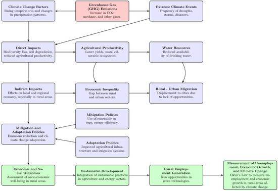
Figure 1.
Effects of climate variability on rural areas and adaptation and mitigation policies. Source: Prepared by the authors.
Among the direct effects, the second line of the figure displays the loss of biodiversity, soil degradation, and the reduction in agricultural productivity. This translates into a decrease in agricultural productivity (e.g., lower yields and more vulnerable ecosystems) and water resources. As indirect effects, the third line of the figure shows economic inequality and migration from rural to urban areas, which feedback into each other between direct and indirect aspects. This is why, as indicated in the fourth line, adaptation and mitigation policies are necessary, including the use of efficient and renewable energies, and improvements to agricultural infrastructure and irrigation systems. To generate these policies, it is necessary to assess well-being in rural areas, integrate sustainable practices in agriculture and the energy sector, and generate new employment opportunities in green technologies. To that end, it is important to measure the effect of climate variability on the relationship between growth and unemployment in rural areas, which are the components most affected by this phenomenon.
4. Data and Methodology
This section describes the methodology for the spatial estimation of the elasticities of Okun’s Law in rural areas of Brazil and Mexico. The first step was to consolidate and organize the data, structuring the information on a quarterly basis from Q3 2012 to Q4 2024. To this end, we built two databases: one related to labor market dynamics in rural areas of Brazil and Mexico, and the other focused on climatic variables, including changes in temperature and milliliter levels of rainfall.
4.1. Data
The dependent variable in this study was the logarithm of the number of unemployed people in rural areas by subnational entity (), constructed from official household surveys. For Brazil, data were obtained from the Pesquisa Nacional por Amostra de Domicílios Contínua (PNADc) provided by the Instituto Brasileiro de Geografia e Estatística (IBGE). For Mexico, data came from the Encuesta Nacional de Ocupación y Empleo (ENOE) published by the Instituto Nacional de Estadística y Geografía (INEGI). In both cases, we used the official definitions of unemployment harmonized across years and adjusted to focus only on rural populations, following the rural/urban classifications established by each country.
The main explanatory variable was the logarithm of real household income (), also taken from PNADc (Brazil) and ENOE (Mexico). All income variables were deflated to constant 2015 prices using the official Consumer Price Index (CPI) from each country. In rural areas, we assume that local economies operate under conditions similar to a closed economy without government intervention. This assumption reflects the limited institutional capacity of these territories, where market linkages and public policy instruments are not sufficiently efficient to influence economic outcomes. Therefore, real household income is employed as a proxy for local production growth, since it directly captures the purchasing power and economic activity of rural households. Changes in income thus provide a consistent measure of the productive performance of these territories (Cardoso López & López Cabrera, 2023, 2025)
In addition, we included the logarithm of the regional average temperature () and the logarithm of rainfall accumulation (). These climate variables were constructed using daily gridded data from the (National Centers for Environmental Information [NCEI], 2025). The daily observations were first transformed into quarterly averages for each rural area and then aggregated to the subnational level. Finally, these values were matched with the household survey microdata using the geographical boundaries of each state or region. The subscript identified each rural area within the states, while referred to the time.
It is worth mentioning that the selection of Brazil and Mexico for this study responded to the importance of both countries within the Latin American and Caribbean region: 57% of regional GDP in 2021 (Gaudin & Pareyón, 2020). In addition, their geographical and climatic diversity made it possible to analyze how climate variability impacted rural areas unequally. Furthermore, the strategic role of the rural sector in their economies, both in terms of agricultural production and food security, and their high vulnerability to climate variability highlighted their relevance. Finally, their different levels of productive diversification offered a useful comparative framework for understanding rural labor dynamics in different Latin American contexts (Comisión Económica para América Latina y el Caribe (CEPAL) & EUROCLIMA+, 2018).
4.2. Econometric Model
This section presents the model used to estimate the short-term elasticities of Okun’s Law and the impacts of climate variability in rural areas of the selected countries. We apply a Spatial Durbin Dynamic Panel (SDPD) model, which captures both temporal and spatial effects in a causal framework (J. Elhorst, 2014). This specification is particularly suitable for addressing serial dependence across geographical units over time, while also accounting for spatial interactions among departments, regions, and states in the countries analyzed (J. Elhorst, 2014; J. P. Elhorst & Emili, 2022).
The SDPD model was recognized for its capability to simultaneously capture spatial dependence and unobservable effects in time and space, also allowing for causal analysis between geographic units (J. P. Elhorst & Emili, 2022). These characteristics were especially useful for studying how economic and climatic variables interacted in rural areas, where spatial and temporal dynamics were decisive in explaining the phenomena.
It should be noted that the Spatial Durbin Dynamic Panel (SDPD) model employed in this study assumes linear relationships between explanatory variables and rural unemployment. This assumption allows for a tractable interpretation of elasticities and facilitates the identification of direct and indirect spatial effects. However, as suggested in the literature, rural labor markets may exhibit nonlinear dynamics, for instance threshold effects in income-employment relationships, asymmetric responses to climatic shocks, or nonlinear spillovers across regions (J. P. Elhorst & Emili, 2022; Baltagi et al., 2007). Exploring these nonlinear dynamics was beyond the scope of the present paper, but it represents an important avenue for future research to more fully capture the complexity of rural labor market adjustments to economic and climatic conditions.
In this study, we used a weight matrix based on Euclidean distances2, where the closest units received greater weights, reflecting greater spatial interdependence. Thus, we applied the kernel grouping method for the efficient selection of neighbors where spatial relationships were shared. This choice allowed us to accurately capture the influence that one geographical unit exerted on another based on its proximity (Cabral et al., 2020; Duran, 2022; J. P. Elhorst & Emili, 2022; Lesage & Pace, 2009). The Dynamic Spatial Durbin Panel (SDPD) regression equation was specified as follows:
where, the dependent variable (the logarithm of the number of unemployed in the rural territory over time ) is a vector of . is a matrix of exogenous variables (the socioeconomic variables of the states and the climatic variables of the rural territories) of dimensions , where represents the number of spatial units and the number of exogenous explanatory variables. Additionally, the subscript refers to the time lagged by a period and represents the spatial weight matrix. Finally, represents the coefficient of spatial lags of the dependent variable. In this sense, the direction and significance condition of the impacts will be evaluated to associate the causal effect of economic and climatic variables on unemployment in a geographical unit and in the associated neighbors.
To ensure valid estimates in dynamic spatial panel models, it was essential to verify the stationarity condition in both the temporal and spatial components. Meeting this condition avoided persistent trends in the variables, reducing the risk of spurious relationships and biases in the results (Baltagi et al., 2003). Additionally, it ensured that spatial dependence between geographical units remained stable over time, which allowed for the identification of dynamic and spatial effects, improved causal interpretation, and minimized problems of collinearity or correlation in errors (Baltagi et al., 2007; J. P. Elhorst & Emili, 2022). For that reason, we applied the Baltagi, Song, and Koh (BSK) test as an alternative hypothesis for the existence of a spatial relationship between the geographical units.
The BSK test is based on the Lagrange Multiplier and the spatially conditioned Lagrange Multiplier (Baltagi et al., 2007). This statistic is constructed from the partial derivative vector of the log-likelihood with respect to the spatial parameters, evaluated under the null hypothesis, and from the inverse of the Fisher information matrix, which reflects the expected information on these parameters. Its general form is , and it allows the validity of models without contrasting spatial effects, and without the need to estimate unrestricted models, being an efficient tool to detect the presence of spatial lags or autocorrelation in errors (Baltagi et al., 2003, 2007).
The conditioned version of the LM statistic adjusts the test to control for the possible simultaneous presence of other spatial effects, evaluating the significance of a specific spatial effect conditional on the fact that the other is already present in the model (Baltagi et al., 2007). Moreover, in this analysis we used the Lagrange Multiplier statistic along with the Hausman test to set the panel effects. In this context, rejection of the null hypothesis favored the fixed-effect model, while non-rejection supported the existence of random effects.
Although robustness checks such as Arellano–Bond tests or fixed effects versus GMM estimators are standard in dynamic panel models, they are not directly applicable to the Spatial Durbin Dynamic Panel (SDPD) framework. Instead, we applied diagnostic procedures suited to spatial dynamic models. Specifically, the Baltagi–Song–Koh (BSK) test confirmed the stability of temporal and spatial components, and the results remained consistent when alternative spatial weight matrices were employed. These checks support the robustness of our findings.
Also, a possible limitation of this analysis is the simultaneity between income and unemployment, which is inherent to the empirical formulation of Okun’s Law and may lead to endogeneity. The SDPD model mitigates this concern through the inclusion of temporal and spatial lags, although it does not fully eliminate it (Cardoso López & López Cabrera, 2023, 2025).
To verify Okun’s Law in rural areas, we examined the sign of the coefficient associated with the real income variable (). We expected a negative value and statistical significance that would corroborate the existence of the rural Okun’s Law both in a specific geographical unit and that of its neighbors (J. P. Elhorst & Emili, 2022). Finally, we analyzed the effects that the explanatory variables exerted on the dependent variable, both within the same spatial unit (direct effects) and through interactions with neighboring units (indirect effects). Thus, once the model was estimated, the matrix of spatial effects was calculated , where and are the coefficients of the original variables and their spatial terms.
Finally, is the coefficient of the spatial lag of the dependent variable. From this matrix, the direct impact is obtained as the average of the trace (), the total impact as the average of the sum of all the elements and the indirect impact as the difference between the two. Direct effects allowed us to understand how a variable directly influenced its immediate context, while indirect effects revealed the spread of these influences to other geographic units, which was crucial for understanding the contagion effect between geographic units (J. P. Elhorst & Emili, 2022). In addition, the temporal dimension allowed for the identification of the short-term causal relationship.
5. Descriptive Statistics
The goal of this section is to show the descriptive statistics used in the two-stage estimation. First, we analyzed the behavior of elasticities related to the number of unemployed people in rural areas, rural real income, temperature, and rainfall levels in the states of Brazil and Mexico. Secondly, we ran a unit root test for panel data using the Phillips–Perron (PP) technique, in order to assess the stationarity of the series. Guaranteeing the stationarity of the panel was essential to avoid heterogeneity problems and ensure the validity of the econometric results.
Thus, Figure 2 presents the maps with the variables used and the corresponding descriptives, showing a high heterogeneity in all study variables between states and even more so between regions in Brazil.3 In the states of the Northeast region, the rural areas showed higher levels of unemployed people with more limited incomes compared to other regions of the country. By contrast, the south, due to its extensive agricultural productive vocation, shows patterns of lower unemployment in rural areas and an increase in the corresponding incomes (Dos Santos et al., 2024). These results showed an inverse pattern between unemployment and real incomes among states in their rural areas. As for weather variables, the north and northeast were characterized by higher levels of precipitation and temperature, in contrast to the south, where these values were lower. These climatic conditions could have had an impact on agricultural productivity and, therefore, on rural income and employment.
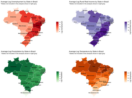
Figure 2.
Spatial Distribution of Average Socioeconomic and Weather Indicators by states’ rural areas in Brazil (in logarithms), Q3 2012 to Q4 2024. * The states not included in the analysis shown un light gray. Source: Prepared by the authors.
Figure 3 displays maps with the variables used and descriptives.4 As can be observed, unemployment in Mexico, in states such as Chiapas, Oaxaca and Guerrero, had the highest elasticities, and, coincidently, showed a greater structural vulnerability in their labor markets. Moreover, these states also had relatively high unemployment levels. By contrast, Baja California, Sonora and Nuevo León showed lower levels, reflecting stronger economic structures and better integration into the formal labor market. This heterogeneity suggested that the effects of economic growth on unemployment varied significantly between states.
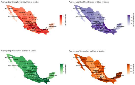
Figure 3.
Spatial Distribution of Average Socioeconomic and Weather Indicators by the states rural areas in Mexico (in Logarithms), Q3 2012 to Q4 2024. Source: Prepared by the authors.
As for real rural income, states such as Yucatán, Quintana Roo, and Campeche reported higher values, although some of these may have been influenced by distortions derived from non-agricultural activities or state interventions, including subsidies or social programs. Otherwise, states such as Zacatecas, Michoacán and Puebla had lower rural incomes, in line with patterns of informality and less access to markets. This contrast reaffirmed the need to understand the behavior of rural income not only in terms of geography, but also in terms of the institutional and productive dynamics of each state.
Weather variables showed that Chiapas, Oaxaca and Veracruz concentrated the highest levels of precipitation, consistent with their location in tropical areas. By contrast, Baja California, Sonora and Coahuila stood out for their dry climate and low levels of rainfall. The average temperature, although less variable between states, tended to be higher in Tabasco, Campeche and Yucatán, and lower in Chihuahua, Zacatecas and Durango. These weather differences, together with economic differences, strengthened the importance of public policies differentiated by territory, aimed at reducing structural gaps and promoting sustainable rural development (Arenas-Wong et al., 2023).
On applying the Phillips-Perron (PP) test for panels to the data from Brazil and Mexico, we observed that the series corresponding to the elasticity of unemployment, temperature and precipitation were stationary throughout the territories analyzed. By contrast, the elasticity of rural real incomes showed no evidence of stationarity in either country. Although this variable was nonstationary, it was retained in the analysis because of its central role in the empirical validation of Okun’s Law. To mitigate potential biases, the model was estimated in elasticities and included a dynamic specification (Spatial Durbin Dynamic Panel), which reduces spurious correlations by capturing both temporal adjustments and spatial dependencies. Thus, the use of real income in the regressions is consistent with the theoretical framework and ensures meaningful interpretation of the income-unemployment relationship (see Table 1).

Table 1.
Phillips-Perron Unit Root Test for Rural Areas of the States Data Panel: Results for Brazil and Mexico, Q3 2012 to Q4 2024.
The descriptive analysis confirmed that rural areas in both Brazil and Mexico are highly heterogeneous, with some states facing deeper structural vulnerabilities in terms of income and unemployment. However, these differences reflect genuine territorial disparities rather than statistical outliers. Visual inspection of the distributions and descriptive statistics did not reveal any extreme observations that could disproportionately drive the results. Instead, the estimated elasticities capture the underlying heterogeneity of rural labor markets, which is consistent with the objectives of this study.
6. Results
Table 2 presents the results of the BSK test, both in its standard and conditioned versions. This test contrasted the null hypothesis of absence of spatial autocorrelation against the alternative of the presence of spatial effects, with the p-value being the criterion to evaluate this dependence. As can be seen, the results confirmed the presence of spatial autocorrelation. Likewise, the results of the Hausman test based on the Lagrange statistics were reported, thereby confirming the existence of random effects in both countries analyzed (Baltagi et al., 2007; J. P. Elhorst & Emili, 2022).
Table 2.
BSK Tests for Spatial Data Panel of the rural areas of the states for Brazil and Mexico, Q3 2012 to Q4 2024 1/.
Additionally, Table 3 presents the results of the estimation of the Spatial Durbin Dynamic Panel with the variables in logarithms using the Okun’s Law model for rural areas. The coefficient represents a spatial elasticity of unemployment: a 1% increase in the number of unemployed in neighboring regions is associated with a 0.205% increase in the number of unemployed in a rural region in Brazil, and 0.174% in Mexico. This result showed the presence of spatial interdependencies in absolute unemployment among rural geographical units.
Table 3.
Coefficient estimates of the Spatial Durbin Dynamic Panel applied in the rural areas of the states of Brazil and Mexico, Q3 2012 to Q4 2024.
The temporary lag in unemployment in rural areas showed a positive and statistically significant effect, indicating a persistent dynamic where past time continued to influence the present. This suggested a limited capacity of the territories to adapt to changes in the labor cycle in the short term. Moreover, spatial relationships revealed a similar pattern: unemployment in neighboring regions also increases the sensitivity of local unemployment. These results differed from those of Cardoso López and López Cabrera (2023), who found that in the case of Okun’s Law in rural areas of Mexico, the transition between cycles of unemployment expansion and contraction took place over a period, and was not persistent over time as in this case.
In the case of the approximation of Okun’s Law in the rural areas of Brazil and Mexico at time t, a counterintuitive relationship was identified between the real rural income of the state with respect to rural unemployment, being positive and significant for both countries. According to (Loría et al., 2022), this positive relationship between unemployment and income might lie in structural distortions in the labor market due to institutional, social, and economic phenomena present in these areas (e.g., high informality, seasonal employment linked to agricultural cycles, limited labor mobility across regions, mismatches between skills and job opportunities, and the influence of social protection programs on labor supply incentives). However, it is important to emphasize that our analysis does not empirically test these underlying distortions, and therefore the result should be interpreted with caution and considered a direction for future research.
By contrast, the temporary lag in real income showed a negative effect, but only in Mexico, which validates Okun’s Law. The results have important implications for economic growth processes in these regions, as they suggested that past periods of economic expansion contributed, in the short term, to the reduction in rural unemployment (Cardoso López & López Cabrera, 2023; Pizzo, 2019).
The results of the spatial lag of in period t in Mexico and Brazil were different. For example, the contemporary spatial effect () was negative and statistically significant (−0.364 ***) in Brazil, but not in Mexico. This indicated that an increase in real incomes from neighboring regions reduced local unemployment. This was due to positive externalities or spillovers from economic activity (J. P. Elhorst & Emili, 2022; Vega & Elhorst, 2014). These aspects could be derived for multiple reasons, such as: (1) an economic spillover effect, where neighboring regions enjoy a boost in their real incomes, thus generating a demand for products in the local activity of the main region (J. P. Elhorst & Emili, 2022); (2) greater mobility of unemployed individuals in the main areas to neighboring rural areas with higher incomes (Vega & Elhorst, 2014); and (3) greater integration between rural areas.
In the case of the effect of both spatial and temporal lags of real incomes in rural areas (), both in Brazil (0.213 **) and in Mexico (−0.435 ***), opposing effects were identified in the dynamics of rural unemployment. In Brazil, an increase in rural real incomes in neighboring regions in the previous period translated into an increase in local rural unemployment, which might have been due to an effect of competition or labor displacement. According to Salvati (2015), these effects could be attributed to the fact that an increase in labor productivity in neighboring rural areas caused imbalances in the economic sectors of the main rural regions, driven by migratory processes. In this context, local firms face difficulties in hiring workers who adapt to the new market conditions, which leads to an increase in rural unemployment (Salvati, 2015). However, in Mexico, the relationship between real income and unemployment is negative, which validates Okun’s Law in rural areas.
When analyzing the effect of temperature in rural areas (), both countries display a negative relationship with rural unemployment. In Brazil, the local temperature showed a negative and significant effect on rural unemployment (−0.123 **), indicating that warmer conditions favor economic diversification in rural areas and, consequently, reduce unemployment (Auffhammer, 2018). In Mexico, the coefficient is also negative (−0.283), pointing in the same direction, but is statistically insignificant.
In the same way, a similar result was perceived considering the immediate lag in temperature in the case of Mexico. Where had a negative effect on unemployment, that is, an increase of 1% in the elasticity of temperature in the past period has an effect of 0.531% in the reduction in the elasticity of unemployment in the current period. This demonstrated the cyclical effect of unemployment when there are variations in temperature, where the effect of climate is much softer than in the long term (Brown et al., 2010; Michel-Villarreal et al., 2019).
For the temporal and spatial lag of temperature, the effects are not consistent across countries. In Brazil, the coefficient is negative (−0.286) and not statistically significant, whereas in Mexico the coefficient is positive (0.388 ***) and statistically significant. This disparity suggested differences in the resilience of the rural labor market to climatic variations in neighboring regions. One possible explanation lay in the different resilience of the labor market in the study region to temperature variations in the surrounding regions. In the case of Brazil, a previous increase in temperature in neighboring regions seemed to generate negative adjustments in local employment (Kumar & Maiti, 2024). In contrast, in Mexico, these increases could have been associated with productive disturbances that amplify the vulnerabilities of rural employment, reflecting less articulation or adaptability between regions (Michel-Villarreal et al., 2019).
Finally, the analysis of the components associated with rainfall elasticity in rural areas revealed a positive and statistically significant effect in both territories of the main zone in the short term. This suggested that extreme increases in rainfall translated into accelerated increases in the number of unemployed people in rural areas. This finding was in line with that of Brown et al. (2010), who argued that both extreme rainfall and its decrease had a substantial negative impact on the economic growth of countries, critically affecting the productive dynamics of the rural sector.
Moreover, this effect was not only manifested temporally but also overlaps spatially: weather shocks in one territory tended to have repercussions on neighboring territories, thus amplifying the impact on rural unemployment in a broader regional context (Brown et al., 2010; Dos Santos et al., 2024). The period analyzed also covers the years of the COVID-19 pandemic. However, unlike in urban areas—where lockdowns and mobility restrictions disrupted labor markets—rural economies in Brazil and Mexico were less affected because many of their core activities, particularly agriculture and food supply, are highly inelastic and had to continue operating (Cardoso López & López Cabrera, 2023, 2025).
However, once the components of the model had been estimated, the direct, indirect and total effects for both countries were calculated. These effects allowed us to capture more accurately the sensitivity of rural unemployment to variations in the explanatory variables, both within the territory analyzed and in its neighboring regions.
Direct effects captured the impact of a variable on unemployment in the same territorial unit, while indirect effects reflect spatial externalities, i.e., the influence between neighboring regions (Table 4). The sum of both constituted the total effect, which represented the overall impact on the space system. This decomposition was key to understanding both the local dynamics of rural unemployment and their territorial interdependencies (J. P. Elhorst & Emili, 2022; Palombi et al., 2017; Perman & Tavera, 2005).
Table 4.
Estimates of Direct, Indirect and Total Effects of Rural Areas in the States of Brazil and Mexico, Q3 2012 to Q4 2024.
According to Pereira (2014) and Palombi et al. (2017), the analysis of the total effects provides a better approximation of Okun’s Law in rural areas of Brazil and Mexico. In Brazil, current real income growth within the same territory is positively associated with rural unemployment, suggesting that higher income does not necessarily translate into more employment, while the lagged effect is negative. For neighboring regions, contemporaneous real income shows a negative association with unemployment, consistent with Okun’s Law, but this relationship reverses when lagged spatial effects are considered. In Mexico, the expected negative relationship of Okun’s Law is confirmed only for lagged real incomes and their spatial effects, since contemporaneous effects remain positive. This reveals a more limited dynamic strongly dependent on the regional context (J. P. Elhorst & Emili, 2022).
In the analysis of the sensitivity of temperature on rural unemployment, a predominance of negative effects was observed in Brazil, both at the local level and in neighboring regions. This suggests that increases in temperature elasticity foster economic diversification processes and reduce seasonal unemployment. In Mexico, the local effects of temperature are also negative, pointing in the same direction as Brazil. However, the spatial effects are positive, indicating that higher temperatures in neighboring regions increase local unemployment and reflect a greater vulnerability of rural labor markets to climatic variations.
The analysis of the sensitivity of rural unemployment to rainfall revealed opposite patterns between Brazil and Mexico. In Brazil, increases in rainfall elasticity, whether local, lagged, or spatial, were associated with higher unemployment, suggesting widespread adverse effects on rural activity. In Mexico, while local rainfall increased unemployment, rainfall in neighboring regions reduced it, possibly due to a spillover effect linked to higher labor demand in adjacent areas (Brown et al., 2010; Palombi et al., 2017).
7. Discussion
Our findings show that income growth in rural areas does not immediately translate into job creation. In both Brazil and Mexico, higher current income is paradoxically linked to higher unemployment, a result that reflects the rigidities of rural labor markets, where informality, seasonality, and weak institutions limit opportunities for stable employment. However, when we look at income with a time lag, the picture changes: past income growth tends to reduce unemployment, and in Mexico this effect is statistically significant. This suggests that rural economies need time to absorb the benefits of growth, and that Okun’s Law remains relevant once these delays are considered. The fact that income growth in neighboring regions also helps reduce local unemployment points to the importance of spillovers and territorial interdependence.
Climate variability adds another layer of complexity. In Brazil, warmer temperatures appear to support diversification and reduce unemployment, while in Mexico the effects are less favorable: temperature increases in nearby regions actually raise unemployment, showing that vulnerability can spread across borders. Rainfall is consistently harmful in both countries, with heavy rains increasing unemployment locally and spilling over into neighboring regions. This demonstrates how climate shocks ripple through rural economies, often amplifying existing fragilities.
Together, these results remind us that rural labor markets in Latin America cannot be understood through economics alone. They are shaped by time, space, and the climate itself. Policies that aim to create jobs and strengthen resilience must therefore go beyond short-term income growth and take into account the lagged benefits of growth, the importance of regional coordination, and the disruptive power of climate shocks.
8. Conclusions
In this article, we evaluate the validity of Okun’s Law empirically, adding the effects of climate variability in rural areas of Brazil and Mexico, from a subnational approach, with emphasis on spatial dynamics using a Spatial and Short-Term Durbin Dynamic Panel. The results show that climate variability exerts a significant and differentiated influence on regional economic performance and the evolution of the labor market, affecting both job creation and the sectoral structure of the rural economy.
Thus, this study contributes certain stylized facts to the estimation process: First, it confirms processes of spatial autocorrelation and persistent dynamic effects on rural unemployment, highlighting the interdependencies of the rural labor market in the context of climate variability. Second, it can be observed that the growth of real incomes at the local level does not imply a significant reduction in unemployment, which suggests the presence of structural rigidities and institutional dysfunctions in these markets;. In contrast, incomes in neighboring regions exert a negative effect on local unemployment, partially corroborating Okun’s Law in a spatial and temporal framework.
Third, weather variables show heterogeneous impacts between Brazil and Mexico. In Brazil, higher local temperatures are associated with a reduction in rural unemployment, consistent with processes of economic diversification. In Mexico, lagged temperature effects also reduce unemployment, but increases in neighboring regions’ temperatures significantly raise local unemployment, reflecting cross-regional vulnerabilities. Finally, rainfall has a positive and statistically significant effect on rural unemployment, both directly and through indirect spatial effects, which shows the regional spread of climate shocks and highlights the absence of climate resilience processes or policies in rural areas of Latin America.
In this context, the results suggest that public policies in rural areas of Brazil and Mexico should consider reducing the negative effects of the lack of economic growth on unemployment, since, as can be seen from the validation of Okun’s Law, economic growth has a negative relationship with unemployment. To do this, the heterogeneous effect of climate variability on unemployment, and the spatial relationship in the territory has to be taken into account. Consequently, there must be a differentiated policy in the face of extreme weather events, as well as efficient territorial coordination between the states and regions of Brazil and Mexico. An example of this type of policy is federal disaster funds, and the relaxation of agricultural credit conditions when faced with a natural phenomenon, among others.
Beyond these empirical results, the main contributions of this article are threefold. First, it extends the analysis of Okun’s Law to rural areas under conditions of high climate vulnerability, a dimension often neglected in the literature. Second, it incorporates spatial and temporal spillovers into the empirical estimation, providing new evidence of how neighboring regions’ dynamics influence local rural unemployment. Third, it highlights the differentiated role of climate variables—particularly rainfall—as key determinants of rural labor market fragility, thereby offering novel insights for designing climate-sensitive employment policies in Latin America.
In terms of limitations, this study faces three constraints that should be acknowledged. First, while the Spatial Durbin Dynamic Panel captures both temporal and spatial dependencies, it assumes linear relationships, and possible nonlinear dynamics (e.g., asymmetric responses to climate shocks or threshold effects) were not explored. Second, the analysis relies on the availability and comparability of subnational labor and climate data, which may restrict the inclusion of other potentially relevant variables such as migration flows or informal employment quality. Third, the focus on Brazil and Mexico, although representative of Latin America, limits the generalizability of the findings to other regions. Future research could address these limitations by employing nonlinear specifications, expanding the dataset to other countries, and incorporating additional socioeconomic variables.
Author Contributions
Conceptualization, D.A.C.L. and T.I.C.A.; methodology, D.A.C.L.; software, D.A.C.L. and T.I.C.A.; validation, D.A.C.L. and Á.L.M.S.; formal analysis, D.A.C.L., T.I.C.A. and Á.L.M.S.; investigation, D.A.C.L.; resources, D.A.C.L.; data curation, D.A.C.L.; writing—original draft preparation, D.A.C.L. and J.A.L.C.; writing—review and editing, D.A.C.L. and J.A.L.C.; visualization, D.A.C.L.; supervision, D.A.C.L. and J.A.L.C.; project administration, D.A.C.L. and J.A.L.C.; funding acquisition, D.A.C.L. All authors have read and agreed to the published version of the manuscript.
Funding
This article was funded by Erasmus+ (ERASMUS-EDU-2023-CBHE, SUREST ERASMUS Project) and by Fundación Universitaria Los Libertadores, under the project “Impact of Climate Change on the Economic Sustainability of Rural Areas in Latin America: Application and Extension of Okun’s Law,” internal call code EAC-04-25.
Informed Consent Statement
Not applicable.
Data Availability Statement
All datasets used in this study are publicly available: household survey microdata for Brazil come from PNAD Contínua (IBGE) IBGE (https://www.ibge.gov.br/estatisticas/sociais/saude/17270-pnad-continua.html, accessed on 10 October 2024); for Mexico from ENOE (INEGI) INEGI (https://www.inegi.org.mx/programas/enoe/15ymas/, accessed on 10 October 2024). Consumer price indices used for deflation are the IPCA from IBGE for Brazil IBGE (https://www.ibge.gov.br/estatisticas/economicas/precos-e-custos/9256-indice-nacional-de-precos-ao-consumidor-amplo.html, accessed on 10 October 2024) and the INPC from INEGI for Mexico INEGI (https://www.inegi.org.mx/temas/inpc/, accessed on 10 October 2024). Climate variables (daily temperature and precipitation) were constructed from the NCEI Global Historical Climatology Network–Daily (GHCN-Daily) data products ncei.noaa.gov.
Acknowledgments
We gratefully acknowledge the support of Erasmus+ (ERASMUS-EDU-2023-CBHE, SUREST ERASMUS Project) and the funding provided by Fundación Universitaria Los Libertadores (code EAC-04-25). Their contributions made this work possible.
Conflicts of Interest
The authors declare that there are no conflicts of interest.
Notes
| 1 | Although there is no clear reference to the term, Stern (2007), in his book, examines the relationship between growth, economic development and climate change, while international organizations have warned of the negative consequences of climate change on agriculture, as well as the result of this on economic growth and development (FAO, 2018; FAO et al., 2021). |
| 2 | The spatial weight matrix was defined using Euclidean distances rather than administrative contiguity because the analysis incorporates environmental variables (temperature and precipitation), whose effects diffuse through geographic space and are not constrained by political borders. Distance-based weights allow for capturing continuous spatial gradients and spillovers that more accurately reflect the environmental and climatic dynamics under study (J. Elhorst, 2014; J. P. Elhorst & Emili, 2022). |
| 3 | Brazil is officially divided into 5 regions: North (Acre, Amapá, Amazonas, Pará, Rondônia, Roraima, Tocantins); Northeast (Alagoas, Bahia, Ceará, Maranhão, Paraíba, Pernambuco, Piauí, Rio Grande Do Norte, and Sergipe); Midwest (Federal District, Goiás, Mato Grosso, Mato Grosso do Sul); Southwest (Espírito Santo, Minas Gerais, Rio De Janeiro, São Paulo); and South (Paraná, Rio Grande do Sul, Santa Catarina) (Benedicto & Marli, 2017). |
| 4 | Mexico does not have official regions. |
References
- Ajanaku, B. A., & Collins, A. R. (2021). Economic growth and deforestation in African countries: Is the environmental Kuznets curve hypothesis applicable? Forest Policy and Economics, 129, 102488. [Google Scholar] [CrossRef]
- Arenas-Wong, R. A., Robles-Morúa, A., Bojórquez, A., Martínez-Yrízar, A., Yépez, E. A., & Álvarez-Yépiz, J. C. (2023). Climate-induced changes to provisioning ecosystem services in rural socioecosystems in Mexico. Weather and Climate Extremes, 41, 100583. [Google Scholar] [CrossRef]
- Armenteras, D., Espelta, J. M., Rodríguez, N., & Retana, J. (2017). Deforestation dynamics and drivers in different forest types in Latin America: Three decades of studies (1980–2010). Global Environmental Change, 46, 139–147. [Google Scholar] [CrossRef]
- Auffhammer, M. (2018). Quantifying Economic Damages from Climate Change. Journal of Economic Perspectives, 32(4), 33–52. [Google Scholar] [CrossRef]
- Baltagi, B. H., Heun Song, S., Cheol Jung, B., & Koh, W. (2007). Testing for serial correlation, spatial autocorrelation and random effects using panel data. Journal of Econometrics, 140(1), 5–51. [Google Scholar] [CrossRef]
- Baltagi, B. H., Song, S. H., & Koh, W. (2003). Testing panel data regression models with spatial error correlation. Journal of Econometrics, 117(1), 123–150. [Google Scholar] [CrossRef]
- Benedicto, M., & Marli, M. (2017). Cinco faces do Brasil. Retratos A Revista Do IBGE, 10(6), 10–12. [Google Scholar]
- Brown, C., Meeks, R., Ghile, Y., & Hunu, K. (2010). An empirical analysis of the effects of climate variables on national level economic growth (p. 5357). Policy research working paper. Available online: https://documents.worldbank.org/en/publication/documents-reports/documentdetail/907171468314700762/an-empirical-analysis-of-the-effects-of-climate-variables-on-national-level-economic-growth (accessed on 18 September 2025).
- Burke, M., Hsiang, S. A., & Miguel, E. (2015). Global non-linear effect of temperature on economic production. Nature, 527, 235–239. [Google Scholar] [CrossRef] [PubMed]
- Cabral, R., López Cabrera, J. A., & Padilla, R. (2020). Absolute convergence in manufacturing labour productivity in Mexico, 1993–2018: A spatial econometrics analysis at the state and municipal level. (Estudios y Perspectivas Sede Subregional de la CEPAL en México 4649).
- Cardoso López, D. A., & López Cabrera, J. A. (2023). Estimación de la Ley de Okun para México al nivel estatal y por tamaño de localidad. Sobre México Temas de Economía, 1(7), 36–83. [Google Scholar] [CrossRef]
- Cardoso López, D. A., & López Cabrera, J. A. (2025). Evidencia empírica de la ley de Okun en Colombia: Un análisis de las zonas rurales a nivel regional. Revista CEPAL, 145. Available online: https://hdl.handle.net/11362/81882 (accessed on 18 September 2025).
- CEPAL. (2020). Balance preliminar de las economías de América latina y el caribe. In Comissão Econômica para a América Latina e o Caribe (1st ed.). Comisión Económica para América Latina y el Caribe (CEPAL). Available online: https://repositorio.cepal.org/bitstream/handle/11362/46501/1/S2000990_es.pdf%0Ahttp://repositorio.cepal.org/bitstream/handle/11362/37344/S1420978_es.pdf?sequence=68 (accessed on 18 September 2025).
- Comisión Económica para América Latina y el Caribe (CEPAL) & EUROCLIMA+. (2018). La economía del cambio climático en América Latina y el Caribe. Una visión gráfica. CEPAL. [Google Scholar]
- Dell, M., Jones, B. F., & Olken, B. A. (2012). Temperature Shocks and Economic Growth: Evidence from the Last Half Century. American Economic Journal: Macroeconomics, 4(3), 66–95. [Google Scholar] [CrossRef]
- Dos Santos, E. A., Piedra-Bonilla, E. B., Barroso, G. M., Silva, J. V., Hejazirad, S. P., & dos Santos, J. B. (2024). Agricultural resilience: Impact of extreme weather events on the adoption of rural insurance in Brazil. Global Environmental Change, 89, 102938. [Google Scholar] [CrossRef]
- Duran, H. E. (2022). Validity of Okun’s Law in a Spatially Dependent and Cyclical Asymmetric Context. Panoeconomicus, 69(3), 447–480. [Google Scholar] [CrossRef]
- Elhorst, J. (2014). Spatial Econometrics. From Cross-Sectional Data to Spatial Panels. Springer. [Google Scholar]
- Elhorst, J. P., & Emili, S. (2022). A spatial econometric multivariate model of Okun’s law. Regional Science and Urban Economics, 93, 103756. [Google Scholar] [CrossRef]
- Estrada-Carmona, N., Hart, A. K., DeClerck, F. A. J., Harvey, C. A., & Milder, J. C. (2014). Integrated landscape management for agriculture, rural livelihoods, and ecosystem conservation: An assessment of experience from Latin America and the Caribbean. Landscape and Urban Planning, 129, 1–11. [Google Scholar] [CrossRef]
- FAO. (2018). Panorama de la pobreza rural en América Latina y el Caribe. In Organizacióm de las Naciones Unidas para la Alimentación y la Agricultura (1st ed.). FAO. Available online: https://linkinghub.elsevier.com/retrieve/pii/S0165176508001857 (accessed on 18 September 2025).
- FAO, European Union & CIRAD. (2021). Food systems assessment—Working towards the SDGs: Interim synthesis brief—September 2021. FAO; European Union; CIRAD. [Google Scholar]
- FAO, IFDA, UNICEF, WFP & WHO. (2023). El estado de la seguridad alimentaria y la nutrición en el mundo: Urbanización, Transformación de los sistemas agroalimentarios a lo largo del continuo rural—Urbano. In El estado de la seguridad alimentaria y la nutrición en el mundo 2023 (1st ed.). FAO; IFDA; UNICEF; WFP; WHO. [Google Scholar] [CrossRef]
- Galbraith, J. K. (2021). The Political Economy of the Apocalypse. Emancipations: A Journal of Critical Social Analysis, 1(1), 1. [Google Scholar] [CrossRef]
- Gasper, R., Blohm, A., & Ruth, M. (2011). Social and economic impacts of climate change on the urban environment. Current Opinion in Environmental Sustainability, 3(3), 150–157. [Google Scholar] [CrossRef]
- Gaudin, Y., & Pareyón, R. (2020). Brechas estructurales en América Latina y el Caribe Una perspectiva conceptual-metodológica. In Cepal. Available online: https://repositorio.cepal.org/bitstream/handle/11362/43405/7/S1800082_es.pdf (accessed on 18 September 2025).
- Gowdy, J., & Salman, A. (2007). Climate change and economic development: A pragmatic approach. The Pakistan Development Review, 46(4), 337–350. [Google Scholar] [CrossRef][Green Version]
- Islam, N., & Winkel, J. (2017). Climate change and social inequality (p. 30). DESA Working Paper No. 152. United Nations. [Google Scholar]
- Jedwab, R., Christiaensen, L., & Gindelsky, M. (2017). Demography, urbanization and development: Rural push, urban pull and … urban push? Journal of Urban Economics, 98, 6–16. [Google Scholar] [CrossRef]
- Jessoe, K., Manning, D. T., & Taylor, J. E. (2018). Climate change and labour allocation in rural Mexico: Evidence from annual fluctuations in weather. The Economic Journal, 128(608), 230–261. [Google Scholar] [CrossRef]
- Kumar, N., & Maiti, D. (2024). Long-run macroeconomic impact of climate change on total factor productivity—Evidence from emerging economies. Structural Change and Economic Dynamics, 68, 204–223. [Google Scholar] [CrossRef]
- Leichenko, R., & Silva, J. A. (2014). Climate change and poverty: Vulnerability, impacts, and alleviation strategies. Wiley Interdisciplinary Reviews: Climate Change, 5(4), 539–556. [Google Scholar] [CrossRef]
- LeSage, J., & Pace, R. K. (2009). Introduction to spatial econometrics. In Introduction to spatial econometrics. CRC Press. [Google Scholar] [CrossRef]
- Liu, L. Q., Pan, D., & Raissi, M. (2025). Macroeconomic effects of climate change: Evidence from Canadian provinces. International Economics, 181, 100572. [Google Scholar] [CrossRef]
- Loría, E., Rojas, S., & Martínez, E. (2022). Ley de Okun en México: Un análisis de la heterogeneidad estatal, 2004-2018. Revista de La CEPAL, 2021(134), 141–160. [Google Scholar] [CrossRef]
- Michel-Villarreal, R., Vilalta-Perdomo, E., Hingley, M., & Canavari, M. (2019). Evaluating economic resilience for sustainable agri-food systems: The case of Mexico. Strategic Change, 28(4), 279–288. [Google Scholar] [CrossRef]
- Mohaddes, K., Ng, R. N. C., Pesaran, M. H., Raissi, M., & Yang, J.-C. (2023). Climate change and economic activity: Evidence from US states. Oxford Open Economics, 2, odac010. [Google Scholar] [CrossRef]
- Mondal, S., Mishra, A. K., Leung, R., & Cook, B. (2023). Global droughts connected by linkages between drought hubs. Nature Communications, 14, 144. [Google Scholar] [CrossRef]
- Nakhle, P., Stamos, I., Proietti, P., & Siragusa, A. (2024). Environmental monitoring in European regions using the sustainable development goals (SDG) framework. Environmental and Sustainability Indicators, 21, 100332. [Google Scholar] [CrossRef]
- National Centers for Environmental Information (NCEI). (2025, February). Climate data online search. Climate Data Online: Daily Summaries. Available online: https://www.ncei.noaa.gov/cdo-web/results (accessed on 18 September 2025).
- Okun, A. (1962). Potential GNP: Its measurement and significance. American Statistical Association, 98–104. [Google Scholar] [CrossRef]
- Otero, A. (2019). El mercado laboral rural en Colombia, 2010–2019 (p. 281). Documentos de Trabajo Sobre Economía Regional y Urbana (DTSERU). Banco de la República. [Google Scholar] [CrossRef]
- Palombi, S., Perman, R., & Tavéra, C. (2017). Commuting effects in Okun’s Law among British areas: Evidence from spatial panel econometrics. Papers in Regional Science, 96(1), 191–210. [Google Scholar] [CrossRef]
- Pereira, R. M. (2014). Okun’s Law, asymmetries and regional spillovers: Evidence from virginia metropolitan statistical areas and the district of columbia (p. 140). Working Paper. Available online: https://economics.wm.edu/wp/cwm_wp140_rev1.pdf (accessed on 18 September 2025).
- Perman, R., & Tavera, C. (2005). A cross-country analysis of the Okun’s Law coefficient convergence in Europe. Applied Economics, 37(21), 2501–2513. [Google Scholar] [CrossRef]
- Pizzo, A. (2019). Literature review of empirical studies on Okun’s Law in Latin America and the Caribbean (pp. 1–30, Issue 252). Employment Working Paper. International Labour Organisation. Available online: https://www.ilo.org/wcmsp5/groups/public/---ed_emp/---ifp_skills/documents/publication/wcms_734508.pdf (accessed on 18 September 2025).
- Salvati, L. (2015). Space matters: Reconstructing a local-scale Okun’s Law for Italy. International Journal of Finance, Insurance and Risk Management, 5(1), 833–840. [Google Scholar]
- Sathler, D., Adamo, S. B., & Lima, E. E. C. (2018). Deforestation and local sustainable development in Brazilian Legal Amazonia: An exploratory analysis. Ecology and Society, 23(2), 30. [Google Scholar] [CrossRef]
- Scott, D., Hall, C. M., & Gössling, S. (2019). Global tourism vulnerability to climate change. Annals of Tourism Research, 77, 49–61. [Google Scholar] [CrossRef]
- Stern, N. (2007). The economics of climate change. Cambridge University Press. [Google Scholar] [CrossRef]
- Thornton, P. K., Ericksen, P. J., Herrero, M., & Challinor, A. J. (2014). Climate variability and vulnerability to climate change: A review. Global Change Biology, 20, 3313–3328. [Google Scholar] [CrossRef]
- Vega, S. H., & Elhorst, J. P. (2014). Modelling regional labour market dynamics in space and time. Papers in Regional Science, 93(4), 819–841. [Google Scholar] [CrossRef]
- Wei, Y., An, M., Huang, J., Fang, X., Song, M., Wang, B., Fan, M., & Wang, X. (2024). How human activities affect and reduce ecological sensitivity under climate change: Case study of the Yangtze River Economic Belt, China. Journal of Cleaner Production, 472, 143438. [Google Scholar] [CrossRef]
- Xu, Z., & Peng, J. (2024). Recognizing ecosystem service’s contribution to SDGs: Ecological foundation of sustainable development. Geography and Sustainability, 5(4), 511–525. [Google Scholar] [CrossRef]
- Zhao, M., Zhu, M., Chen, Y., Zhang, C., & Cai, W. (2024). The uneven impacts of climate change on China’s labor productivity and economy. Journal of Environmental Management, 351, 119707. [Google Scholar] [CrossRef]


Disclaimer/Publisher’s Note: The statements, opinions and data contained in all publications are solely those of the individual author(s) and contributor(s) and not of MDPI and/or the editor(s). MDPI and/or the editor(s) disclaim responsibility for any injury to people or property resulting from any ideas, methods, instructions or products referred to in the content. |
© 2025 by the authors. Licensee MDPI, Basel, Switzerland. This article is an open access article distributed under the terms and conditions of the Creative Commons Attribution (CC BY) license (https://creativecommons.org/licenses/by/4.0/).