Productivity and Wages in South Africa

Abstract

The world has experienced rapid productivity growth in the last three decades, but has this growth reflected in wages? In theory, under certain conditions, workers earn their marginal product so that productivity growth feeds into wages on a one-to-one basis. Given the contradictory literature, this paper revisited the productivity–wage relationship in South Africa using an industry-level panel dataset comprising 74 industries observed between 1993 and 2023. Using several estimators, four main findings are observed. First, productivity is found to have grown faster than wages. Second, the observed productivity–wage divergence partly reflects the squeezing of workers for profits. Third, productivity growth mostly outpaced the wages of low-skilled workers, workers on short-term contracts, and informal workers. Fourth, productivity growth largely undermined take-home pay compared to fringe benefits. These results imply that although boosting productivity growth may be important, its achievement may not lead to broad-based wage gains in South Africa unless the government pursues policies that realign productivity and the pay of low-skilled workers, informal workers, and workers on short-term contracts. Such policies may include sector-based incentives for businesses that improve wage conditions, increased union support in high-growth industries, improved regulation of the informal sector, and vocational training for low-skilled workers.

1. Introduction

Economic theory predicts that workers in competitive markets are paid their marginal product such that growth in labour productivity feeds entirely into real wages on a one-to-one basis. In contrast to this prediction, real wages have failed to keep pace with labour productivity globally in the last three decades (Feldstein 2008; Mishel 2012; Stansbury and Summers 2018). In some studies, it is suggested that the relationship between labour productivity and wages may have broken.

This paper revisits this discussion by estimating the short- and long-term impact of labour productivity on real remuneration in South Africa. It aims to unravel the heterogeneities in the productivity–wage relationship between (i) low-, semi-, and skilled workers and (ii) formal and informal workers. In addition to the commonly used remuneration per worker proxy for labour income, it seeks to separately establish the potential heterogeneous impact of productivity on wages and benefits. In a bid to establish the underlying factors influencing the productivity–wage relationship, the paper determines the extent to which the expansion of industrial profits may have prevented productivity from raising labour income in South Africa between 1993 and 2023.

Within the literature, the empirical findings have largely been inconclusive. In Dostie (2011), for instance, the conclusion is that wages do not deviate significantly from productivity, suggesting a near one-to-one relationship. This result is similarly observed in the studies by Van Biesebroeck (2003) and more recently Herman (2020). However, the relationship between productivity and wages is found to be either weak, non-existent, or less than one-to-one. Schwellnus et al. (2017) particularly find aggregate labour productivity growth in most OECD countries to have decoupled from the real median compensation growth. Their observation suggests that increasing productivity may not sufficiently raise real wages for the typical worker in the region.

Despite the vastness of the literature linking productivity with wages, only Wakeford (2004) and Tsoku and Matarise (2014) have, to our knowledge, explicitly examined the short-run and long-run impact of productivity growth on real remuneration in the context of South Africa. These studies reached conflicting conclusions. Wakeford (2004) concluded that labour productivity in South Africa feeds into wages only in the long run, and it does so on a less than one-to-one basis, while Tsoku and Matarise (2014) concluded that productivity growth does not significantly feed into wages using a specification comprising real remuneration, productivity, and the rate of unemployment.

This paper differs from the above studies in several ways. First, it categorises labour into (i) formal and informal workers and (ii) low, semi-skilled, and skilled workers. These decompositions allow us to provide a clearer picture of how the real earnings of specific groups responded to productivity dynamics during the sampling period. Second, in addition to the commonly used real remuneration measure, it distinguishes between real wages and real benefits. Wages differ from remuneration in that they exclude employer contributions for social insurance, pension contributions, and employer payments for health insurance and other fringe benefits (Bosworth et al. 1994). From a research standpoint, Cashell (2004) argues that the use of wages while ignoring benefits can be empirically misleading as the two evolve at different paces. From a policymaking viewpoint, the heterogeneous evolution of wages and benefits may have different welfare implications.

As recommended by Wakeford (2004), this paper pursues a disaggregated approach that uses data on 74 industries. The dataset comprises all three sectors of the economy, namely, primary, secondary, and tertiary. The total sample particularly comprises 3 industries from the agricultural sector, 7 from mining, 42 from manufacturing, and 22 from services. This disaggregated approach enables us to exploit the rich variation in productivity growth and wages across industries belonging to different sectors in a bid to attain a reflective picture of how and why wages may have decoupled from productivity growth in South Africa. The accommodation of sectoral and industrial diversity is important, as Faggio et al. (2010) show that focusing on one sector, the manufacturing sector, as did Herman (2020), may underestimate the wage and productivity divergence.

In addition, this paper not only controls for unemployment but also import penetration and export intensity. The literature has shown that trade can influence both productivity growth and wage dynamics; hence, the omission of import penetration and export intensity may lead to an omitted variable bias. Lastly, it considers, in an additional specification, gross markup as an additional control variable. The gross markup of an industry is the net operating surplus as a percentage of total intermediate inputs plus labour remuneration. Since it proxies industrial profits, its inclusion allows us to make inferences about the underlying causes of a less than one-to-one relationship between productivity and wages. A less than one-to-one relationship when gross markup is controlled for would, for example, suggest the presence of other underlying factors besides the expansion of industrial profits preventing productivity growth from fully reflecting in wages. A less than one-to-one relationship that turns one-to-one once gross mark is controlled for would suggest that productivity growth may have been largely prevented from raising wages fully by the expansion of profits.

Having ruled out the possibility of simultaneity through panel Granger causality tests, the empirical analysis was grounded in a standard theoretical framework in which wages are a function of labour productivity and workers are paid their marginal products when markets are competitive. The paper augmented this function with additional controls in a bid to isolate the effect of productivity on wages. Considering the large time dimension and the large number of industries in the sample coupled with the desire to estimate the productivity–wage relationship in the short run and long run, the analysis applied the Pooled Mean Group (PMG) of Pesaran et al. (1999), which accommodates short-run heterogeneity and imposes long-run homogeneity. Potential endogeneity likely to arise from measurement error and third factors nested in the error term was addressed in robustness exercises through the Panel Dynamic Ordinary Least Squares (PDOLS) method and the Panel Fully Modified Ordinary Least Squares (PFMOLS).

The rest of the paper is organised as follows. Section 2 reviews the productivity–remuneration divergence by sector and the theoretical and empirical literature. Section 3 describes the data and specifies the empirical models. The results are presented and interpreted in Section 4. Section 5 concludes the analysis, discusses the policy implications of this study, and suggests areas for further research.

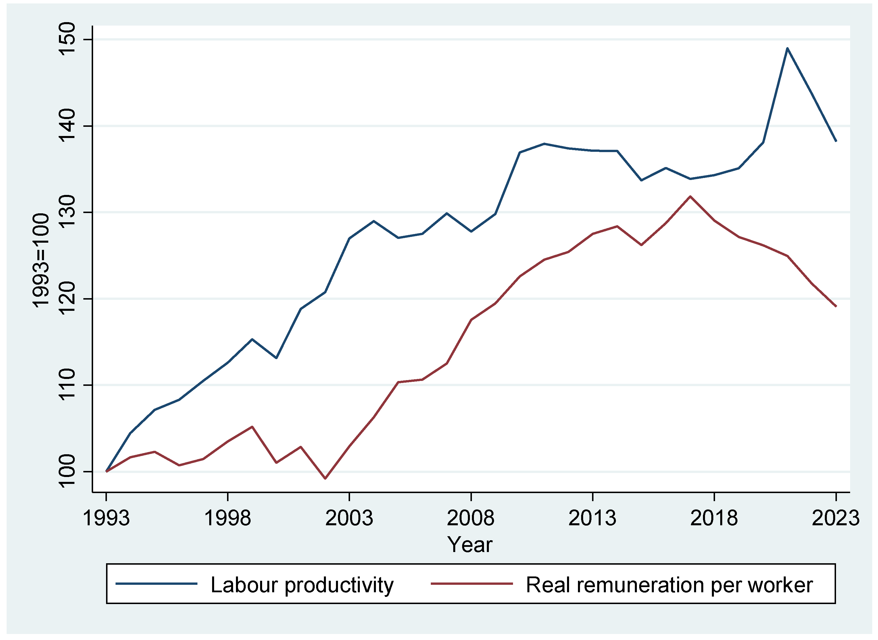
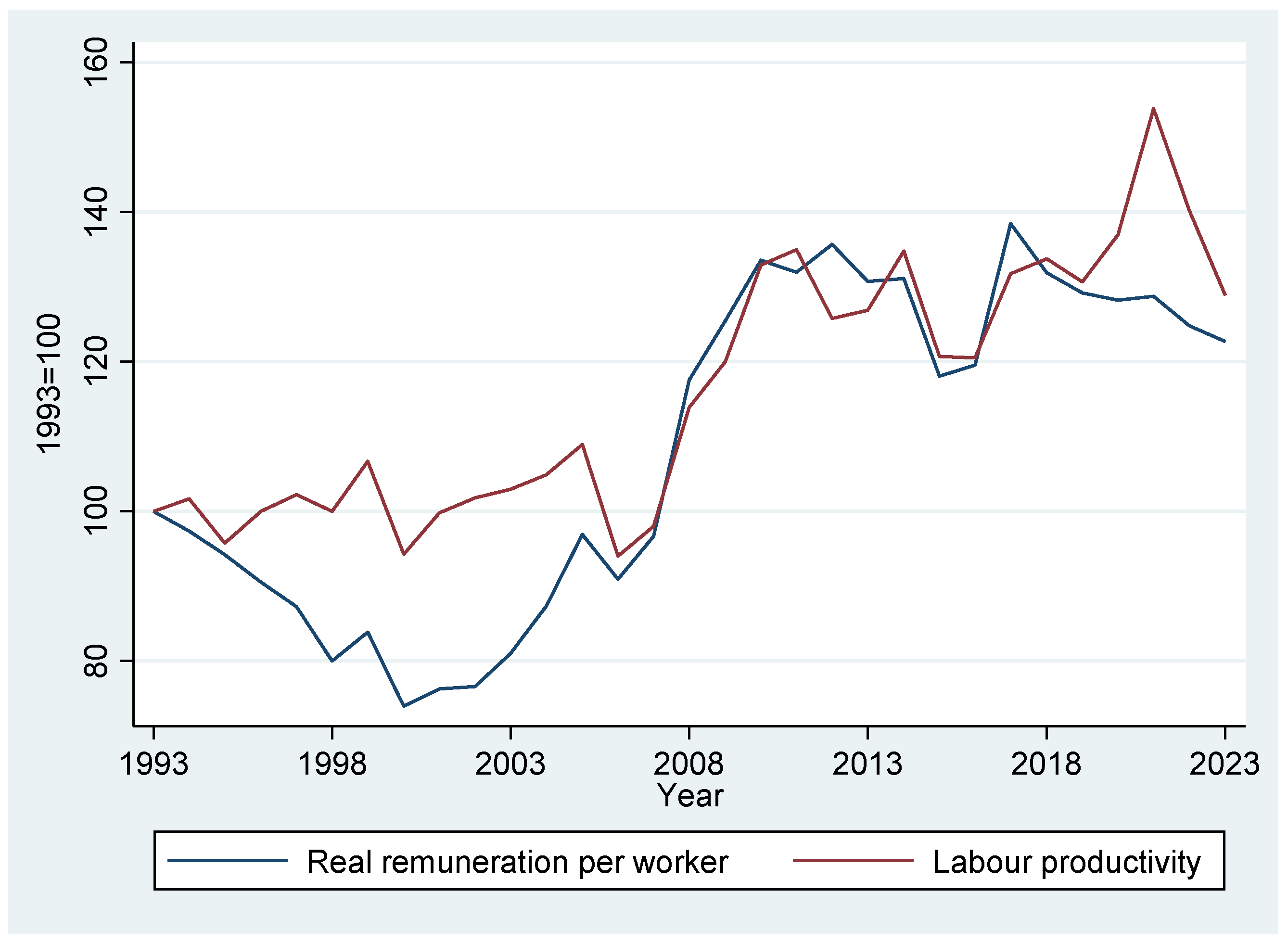
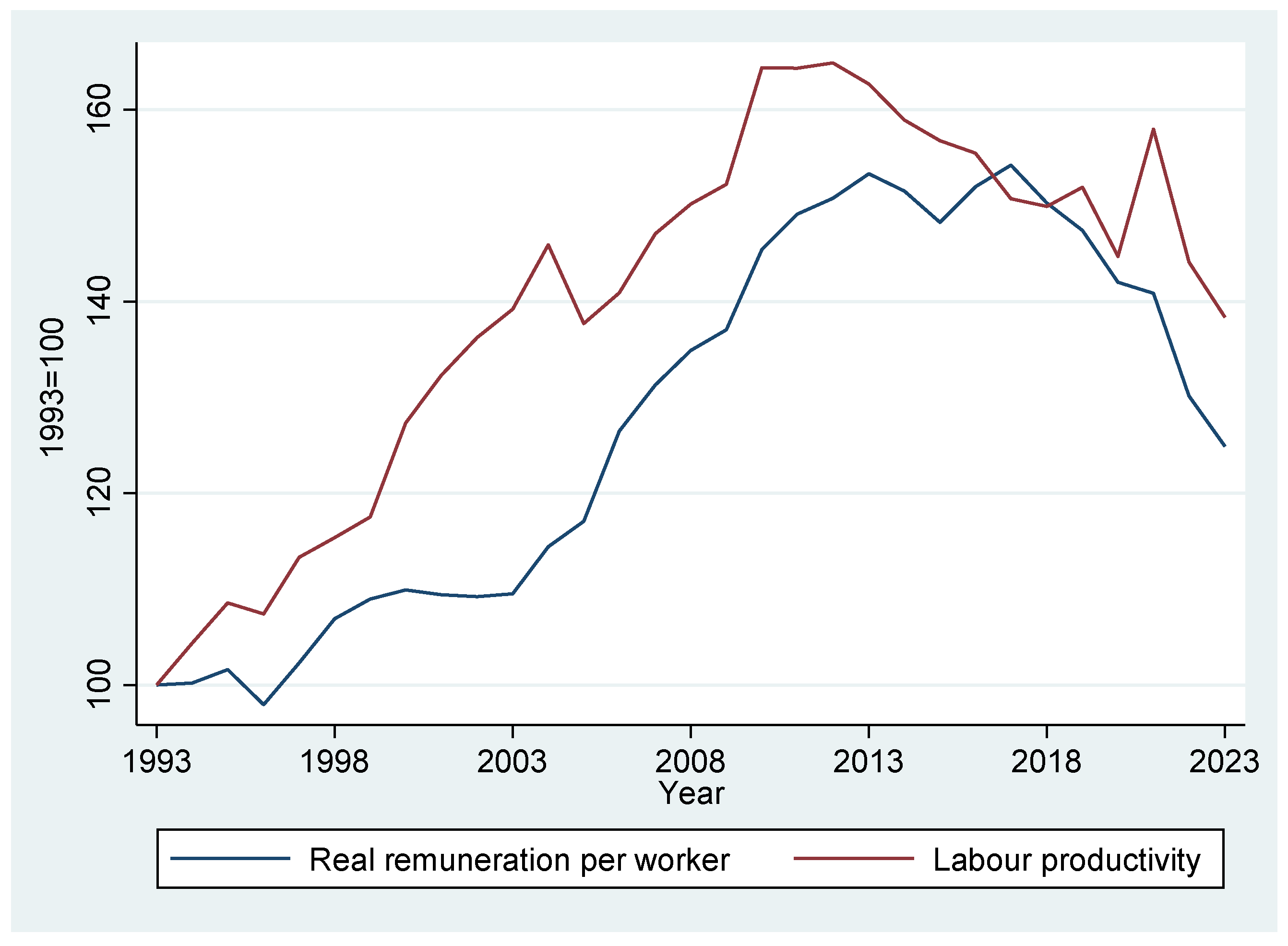
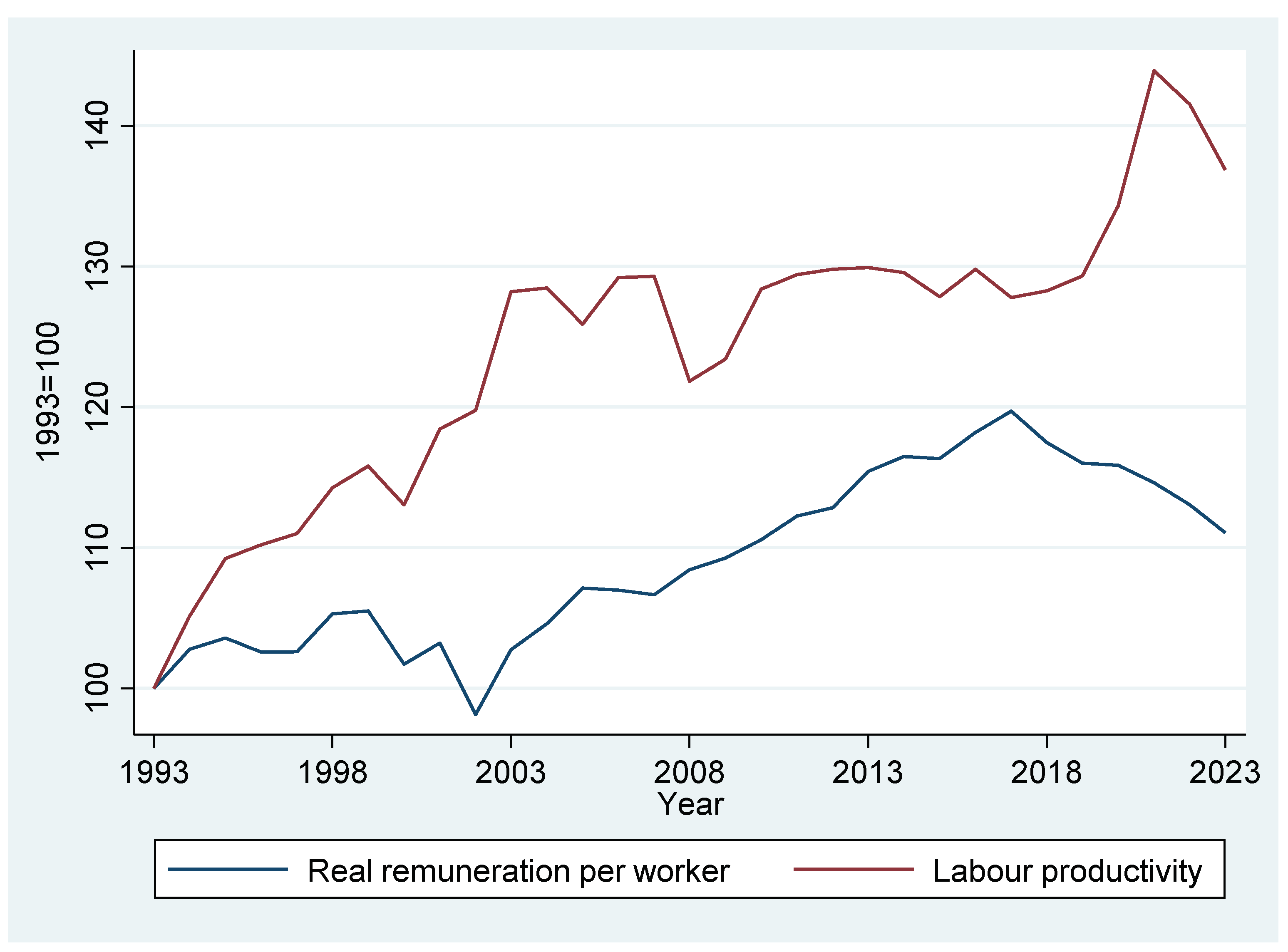
2. The Decoupling of Productivity and Remuneration in South Africa: Stylised Facts

Figure 1 displays the evolution of productivity and real remuneration for all sectors between 1993 and 2023. A cursory look at the graph shows that labour productivity grew faster than real remuneration during the sampling period.

In the primary sector (Figure 2), the decoupling of productivity and real remuneration mostly occurred during the 1993–2006 period and the 2018–2023 period. Between 2007 and 2018, productivity and wages moved closely. In a few instances (2011, 2012, and 2016), real remuneration outpaced labour productivity growth. The general trends in Figure 2, however, mask the heterogeneities across primary sectors. Wages in agriculture, for example, tend to be lower compared to other sectors. This is partly due to the seasonal and often labour-intensive nature of the work, as well as the overall lower value-added in many agricultural activities. Although theory predicts a strong connection between wages and productivity growth, wage increases in South Africa’s agriculture sector have often been modest due to market pressures, low margins, and challenges in passing on higher production costs to consumers. Wages in the mining sector, however, are generally higher compared to the agriculture sectors, reflecting the specialised skills required and the hazardous nature of the work. In the forestry sector, wages are generally moderate, reflecting the skill levels required and the nature of the work. Forestry work is often less mechanised compared to mining, which impacts productivity and wage levels.

Figure 3 displays the evolution of productivity and real remuneration in the secondary sector. A robust secondary sector contributes to industrialisation, which is essential for economic diversification. It reduces dependency on primary sectors like mining and agriculture, which are more vulnerable to external shocks and price fluctuations. Apart from 2017, secondary sectors saw labour productivity divergence from real remuneration during the sampling period. Much of the divergence was observed between 2001 and 2005. From 2006, real remuneration slowly narrowed the gap before slightly exceeding productivity growth, albeit temporarily in 2017. These trends may vary across sectors. Construction workers, for instance, earn moderate wages, with higher pay for specialised roles and managerial positions. Manufacturing wages, on the other hand, are higher compared to agriculture but can be lower than those in high-tech industries.

Tertiary sectors have the largest contribution to gross domestic product (GDP) in South Africa. These sectors saw the largest decoupling of productivity and wages between 1993 and 2023. In 2023, they accounted for 57 percent of total GDP compared to the 31 percent and 12 percent contributions of secondary and primary sectors, respectively. The largest contribution, coupled with the largest productivity and real remuneration divergence (Figure 4), therefore implies that tertiary sectors may have had a significant bearing on overall income inequality in the South African economy between 1993 and 2023. Within the tertiary sector, financial services experienced significant productivity growth, driven by advancements in technology, such as digital banking, fintech innovations, and automation of routine tasks.

Wages in financial services are generally high compared to other sectors, reflecting the specialised skills required and the sector’s profitability. Roles in investment banking, financial analysis, and management tend to command particularly high salaries. In the retail sector, productivity improved through technology adoption, such as e-commerce platforms, supply chain management systems, and inventory automation. Notwithstanding the productivity growth, the retail sector continues to face several challenges, ranging from fluctuating consumer demand and high competition to the need to adapt to changing technology and supply chain disruptions due to power shortages.

In what follows, the analysis describes data and specifies the empirical models.

Literature Review

In detail, the relationship between productivity and wages can be explained using the marginal productivity theory of wages. The marginal productivity theory of wages posits that wages are determined by the marginal productivity of labour. In a competitive labour market, employers will pay workers a wage equal to the value of their marginal product. This ensures that labour is compensated fully based on its contribution to the company’s revenue.

The theory can be used to explain wage differentials across industries based on differences in the marginal productivity of workers. Workers in industries with higher marginal productivity will earn higher wages compared to workers employed in industries with lower marginal productivity. For instance, highly skilled workers in mining industries are more likely to earn higher wages due to their higher marginal productivity compared to workers employed in the clothing industry.

Despite being simplistic and intuitive, the marginal productivity theory of wages has hardly lived up to expectations for a variety of reasons. One of its key weaknesses is the assumption of a perfectly competitive labour market where employers and workers have complete information and there are no barriers to entry or exit. Labour markets often have imperfections, which may prevent a full pass-through effect of productivity to wages.

The above argument is especially relevant in the South African context, where the labour market is mostly dual and characterised by structural barriers that make it rigid. South Africa’s labour market is particularly characterised by formal and informal sectors, limited labour mobility, regulatory challenges, and a skills gap.

The formal labour market in South Africa typically enjoys strong labour protections, including minimum wage laws, social security benefits, healthcare, and retirement plans. Employment contracts are legally binding, and workers are entitled to dispute resolution through established legal frameworks. The formal sector is also characterised by higher wages and better working conditions compared to the informal sector, although the sector continues to suffer the country’s widespread challenges, which include skills gaps and limited job opportunities.

In stark contrast, the informal labour market is marked by low-wage, unstable, and often unprotected forms of employment. This sector includes activities such as domestic work, street vending, casual labour, and other forms of self-employment. Workers in the informal sector generally lack access to formal contracts, social security, healthcare, or other employment benefits. The informal sector is largely unregulated; hence, workers in this sector tend to face precarious conditions, such as inconsistent work hours, lack of legal protection against unfair dismissal, and limited job security.

Another competing theory is the efficiency theory of wages, which, unlike the marginal theory of wages, posits a unidirectional causality that runs from wages to labour productivity. According to the efficiency wage theory, employers, for various reasons, will pay above the market-clearing rate to drive productivity growth (Wu and Ho 2012). The contradictions between the marginal productivity theory of wages and the efficiency theory of wages demonstrate the need for empirically testing the direction of causality before running single-equation models.

Empirical literature linking productivity and wages has significantly evolved over the years from earlier studies such as Davis and Hitch (1949) and Bosworth et al. (1994) to the more recent literature. The contradiction of findings has led many to consider heterogeneities in the relationship ranging from the formality or informality of labour, the skills, and the distinction between long-run and short-run periods.

In Strauss and Wohar (2004), the long-run relationship between real wages and average labour productivity is considered at the industry level for a panel of 459 US manufacturing industries observed between 1956 and 1996. Results reject both cointegration and a one-to-one relationship between productivity and wages. An increase in labour productivity is found to increase wages by less than unity. In Mahlberg et al. (2013), the age-based wage and productivity differentials are considered in the context of Canada using data observed between 1999 and 2005. Observed in their empirical analysis is that wages do not significantly deviate from productivity, indicating a near one-to-one relationship.

Using data from sub-Saharan countries, Van Biesebroeck (2003) found a one-to-one relationship between wages and productivity in specific countries (Zimbabwe) and a less than unity association in countries such as Kenya. In Tanzania, the author could not find any link between wages and productivity. Konings and Marcolin (2014) simultaneously estimate the impact of productivity on wages using city-level data observed between 2005 and 2023. They find the presence of a wage-productivity divergence gap for Brussels and Wallonia. Mawejje and Okumu (2018) specifically focused on African manufacturing industries. Controlling for endogeneity, their main result is that wages reflect labour productivity and the skill of workers.

More recently, in the context of the Organisation for Economic Co-operation and Development (OECD), Cruz (2023) estimated the impact of labour productivity on real wages and employment. The author specifically sought to test the competing theories on wages and productivity, namely, the marginal productivity theory and the efficiency theory of wages. Using a panel dataset comprising 25 OECD economies, the author finds a positive bidirectional causality between labour productivity and real wages. This result validates the efficiency wage theory, in which changes in wages can also influence labour productivity.

In Cirillo and Ricci (2022), a firm-level dataset is employed. Results from different quantile regression models driven by the desire to capture distributional effects of productivity growth show that labour productivity is in fact negatively associated with wage growth. The negative association between labour productivity and wages is found to decrease in magnitude along the quantiles. These results demonstrate the empirical ambiguity characterising the relationship between productivity and wages.

In the context of South Africa, Wakeford (2004) examines the association between labour productivity and average real wages at the macro level. Using an annual time series dataset, a long-run wage–productivity elasticity of 0.58 is confirmed, validating the productivity–wage divergence. Tsoku and Matarise (2014) similarly estimated the impact of productivity on real remuneration. Their results reject the efficiency theory of wages, as real remuneration is found not to affect Granger causality results in labour productivity.

This paper adds to the above empirical evidence by employing an industry-level analysis that comprises industries from all sectors of the economy. It additionally decomposes labour by formality and skills. Lastly, it decomposes labour income into real wages and real benefits.

3. Materials and Methods

This section presents the methods utilised to achieve the aim of this study. The section specifically describes the data, outlines the estimation strategy, and specifies the empirical model.

3.1. Data and Variables

The analysis uses a macro-panel dataset comprising 74 three-digit industries (N = 74) observed annually from 1993 to 2023 (T = 31). This implies a macro-panel dataset with 2294 annual observations. Data on all variables are sourced from Quantec. Quantec is a consultancy firm providing economic and financial data, country intelligence, and quantitative analytical software, based in Pretoria, South Africa. It has been a source of data for prominent studies such as Rodrik (2008) and Jenkins (2008). From this data source, the analysis draws data on real remuneration per worker deflated using 2015 output prices, labour productivity (for formal and informal workers and low-skilled, semi-skilled, and skilled workers), import penetration, and export intensity. By definition, real remuneration per employee (w) is equal to the total compensation of employees (C) divided by the number of employees (N), that is, w = C/N. Unit labour cost is equal to wage rate or earnings per worker (w) times the number of workers (N) divided by the output produced by the workers (Q), that is, (w × N)/Q, where w × N is a measure of the cost of labour. This means that with remuneration per worker and unit labour costs, we can algebraically split labour income into benefits and wages per worker.

The data source categorises workers into low-skilled, semi-skilled, and skilled workers. These categories can be further categorised into formal and informal workers. Skilled formal sector employment comprises formal sector managers, professionals, and technicians, and it particularly includes professional, semi-professional, and technical occupations; managerial, executive, and administrative occupations; certain transport occupations; and pilot navigators. Semi-skilled formal sector employment comprises formal sector clerks, sales and services, skilled agriculture, crafts and related trade, plant and machine operators, and it particularly includes clerks, service workers and shop and market sales workers, skilled agricultural and fishery workers, craft and related trades workers, plant and machine operators, and assemblers. Low-skilled formal sector employment comprises formal sector elementary work and domestic workers. It includes elementary occupations, domestic workers, and other occupations.

Formality and informality of labour is measured systematically. First, Quantec derives its employment data from the two main official sources of labour data in South African the Quarterly Employment Statistics (QES) and the Quarterly Labour Force Survey (QLFS) published by Statistics South Africa (Stats SA). The QES data are collected from a sample of non-agricultural enterprises and provide a formal employment figure. This figure also excludes domestic workers. The QLFS is a household-based survey and provides figures for total formal and informal employment as well as the official unemployment figure. To bridge the discrepancy between the formal employment figures from these datasets, Quantec uses the QES formal figure, to which it adds formal agricultural and domestic workers. Using the total employment from the QLFS, informal employment is calculated as a residual. Labour productivity is the ratio between output (Q) and the labour input (LI) used to produce that output, that is, labour productivity = Q/LI = output per unit of labour input. It is therefore essentially output per worker obtained from dividing total output by the total number of workers employed.

The import–domestic demand ratio, or import penetration, is equal to total imports (Z) divided by total domestic demand (DD) times one hundred, that is, the import–domestic demand ratio = (Z/DD) × 100. Domestic demand is equal to total output plus imports minus exports. The import–domestic demand ratio is an indication of how much of the domestic demand is satisfied by imports. The export-output ratio is a measure of how much of a country’s output they export. The export-output ratio is equal to total exports (X) divided by total output (Q) of an economy multiplied by one hundred, that is, the export-output ratio = (X/Q) × 100. Lastly, we consider gross markup as an additional control variable. The gross markup of an industry is the net operating surplus of that industry as a percentage of total intermediate inputs plus labour remuneration for that industry. It is a measure of industrial profits.

3.2. Estimation Strategy

The choice of an appropriate baseline strategy was narrowed to estimation approaches that are suitable when both N and T are quite large, as research into the asymptotics of macro-panels has raised the need for considering slope heterogeneity (Phillips and Moon 2000; Im et al. 2003) and non-stationarity under this circumstance. Both aspects suggest that the traditional fixed-effects or random-effects and instrumental variable approaches may not be appropriate in the present case given that N and T are quite large, N = 74 and T = 31, and non-stationarity could be problematic. The alternative approach of averaging the annual observations into 5-year averages to eliminate business cycle effects is less desirable for a variety of reasons. First, it is associated with a loss of information as the transformation directly distorts the original underlying data-generating process. Second, it is also not obvious that average completely eliminates cyclical effects. Third, averaging will take away the ability to separate short-run and long-run effects of productivity on wages.

Common approaches designed for large N and large T cases are the dynamic fixed effects (DFEs), in which the time-series data for each group are pooled and only the intercepts are allowed to differ across groups; the Mean Group (MG) estimator, in which the intercepts, slope coefficients, and error variances are all allowed to differ across groups; and the Pooled Mean Group (PMG) estimator, which is an intermediate estimator to the extent that it allows short-run heterogeneity (as would the MG estimator) and imposes long-run slope homogeneity (as would the DFE). It is standard to determine the more appropriate estimator between the three using a Hausman specification test (Blackburne and Frank 2007). As the results will later show, the PMG approach was preferred.

The PMG approach is a single-equation approach, and its application may be criticised in cases where bidirectional causality cannot be ruled out. This is especially relevant in this paper given the efficiency theory of wages, which treats productivity as a function of wages and not the other way around. The efficiency theory of wages particularly argues that the productivity of workers depends positively on their wages (Leibenstein 1957; Shapiro and Stiglitz 1984; Katz 1986). Preliminary panel Granger causality results found causality running from real remuneration to labour productivity and not the other way around; hence, we could safely proceed with the single-equation PMG approach without the risk of simultaneity.

To illustrate the mechanics underpinning the PMG estimator, suppose we have data on a number of time periods, $t=1,\dots , T,$ and a number of groups $i=\mathrm{1,2},3,\dots , N$, and wish to estimate an ARDL $(p,q,q,\dots , q)$ model as follows:

$$y_{it}=\sum _{j=1}^p{\lambda }_{ij}{y}_{i,t-j}+\sum _{j=0}^q{\delta }_{ij}^{\prime }{x}_{i,t-j}+u_i+{ϵ}_{it}$$

(1)

where the number of groups $i=1, 2,\dots N$; the number of periods $t=1, 2,\dots T$; $x_{it}$ is a $k\times 1$ vector of explanatory variables; ${\delta }_{ij}$ are the $k\times 1$ coefficient vectors; ${\lambda }_{ij}$ are scalars; and $u_i$ is the group-specific effect.

If the variables in $\left(1\right)$ are $I\left(1\right)$ and the error term is an $I\left(0\right)$ structure, then cointegration exists, and any deviation from the equilibrium level will be restored through an error-correction process. In this case, it is common to reparameterise (1) into the error-correction equation as follows:

$$∆y_{it}={\varphi }_i(y_{it-1}-{\theta }_i^{\prime }{x}_{it})+\sum _{j=1}^{p-1}{\lambda }_{ij}^{\mathrm{*}}{∆y}_{i,t-1}+\sum _{j=0}^{q-1}{\delta }_{ij}^{\mathrm{*}\prime }{∆x}_{i,t-j}+u_i+{ϵ}_{it},$$

(2)

$${\varphi }_i=-\left(1-\sum _{j=1}^p{\lambda }_{ij}\right),{\theta }_i=\sum _{j=0}^q{\displaystyle \frac{{\delta }_{ij}}{(1-\sum _k{\lambda }_{ik})}}, {\lambda }_{ij}^{\mathrm{*}}=-\sum _{m=j+1}^p{\lambda }_{im},i=\mathrm{1,2},\dots , N; t=\mathrm{1,2},\dots , T;$$

$${\delta }_{ij}^{\mathrm{*}}=-\sum _{m=j+1}^q{\delta }_{im}, j=1,\dots , p-1$$

(3)

where ${\varphi }_i$ is the error-correction term, which is expected to be significantly negative and ideally lie between 0 and 1 in absolute terms under the assumption of cointegration.

3.3. Empirical Model

The empirical model employed in this paper builds on the theoretical framework applied in Mawejje and Okumu (2018). Consider that firms ($i,\dots , N$) across the industries use labour (L), capital (K), and government by technology (A) to produce a homogenous product (Y). Labour is heterogeneous in formality and skills. A Cobb–Douglas representation of each firm with constant returns to scale can be specified as follows:

$$Y_{it}=A{K}_{it}^{\alpha }{L}_{it}^{\beta }$$

(4)

where i denotes the firm, t represents the time, and $\alpha$ and $\beta$ are factor shares. The function is assumed to be twice differentiable with positive marginal products and diminishing marginal rates of substitution. Labour is paid a wage (w), while capital earns a return (r).

The profit (${\pi }_{it}$) function is given as follows:

$${\pi }_{it}=A{K}_{it}^{\alpha }{L}_{it}^{\beta }-w_{it}{L}_{it}-r_{it}{K}_{it}$$

(5)

Profit maximisation, therefore, implies the following:

$$w_{it}=\beta A{K}_{it}^{\alpha }{L}_{it}^{\beta -1}$$

(6)

Defining labour productivity, ${LP}_{it}$, as output per unit labour, that is, ${LP}_{it}={\displaystyle \frac{Y_{it}}{L_{it}}}$, the wage function can be specified as follows:

$$w_{it}=\beta {LP}_{it}$$

(7)

Differentiating Equation (4) with respect to LP gives us the marginal effect of labour productivity on wages such that

$${\displaystyle \raisebox{1ex}{$\partial w_{it}$}\!\left/ \!\raisebox{-1ex}{$\partial {LP}_{it}$}\right.}=\beta >0$$

(8)

Expression (5) implies a positive association between labour productivity and wages. A one-to-one relationship would be confirmed by $\beta =1$. The literature, however, emphasises the importance of adding control variables to isolate the impact of productivity on wages. In this paper, trade variables, the rate of unemployment, and gross markup are added to Equation (7). The final estimated model then takes the following form:

$$\log y_{it}={\theta }_{0i}+{\theta }_{1i}{\log prod}_{it}+{\theta }_{2i}{im}_{it}+{\theta }_{3i}{ex}_{it}+{\theta }_4{unem}_t+{ϵ}_{it}$$

(9)

$$i=1,\dots , 74; t=1993,\dots , 2023$$

where log denotes logarithm (i.e., base 10), $i$ is the industry, $t$ is the year, and $y_{it}$ is the real remuneration per worker (2015 = 100) in the first estimation, wage per worker in the second and benefits per worker in the third; $prod$ is the labour productivity; $im$ is the import penetration; $ex$ is the export intensity;$unem$ is the unemployment rate, which varies over time but not across industries; ${\theta }_1-{\theta }_4$ are the unknown parameters to be estimated through the maximum likelihood estimator; and $ϵ$ is the error term. If productivity feeds into wages, or more appropriately, remuneration on a one-to-one basis, then ${\theta }_{1i}=1,$ which is testable post-estimation. Imports and exports can have negative or positive effects on real remuneration. If trade increases labour demand and ultimately wages for a typical worker, then ${\theta }_{1i},{\theta }_{2i}>0$. If trade lowers labour demand and reduces real remuneration for a typical worker, then ${\theta }_{1i},{\theta }_{2i}<0$ otherwise ${\theta }_{1i},{\theta }_{2i}=0$.

The estimated baseline model was a panel ARDL (1, 1, 1, 1, 1) selected automatically by the Akaike Information Criterion (AIC) from a maximum of 2 lags. The equation corresponding to this specification is as follows:

$$\log y_{it}={\theta }_{11i}{\log prod}_{it}+{\theta }_{12i}{\log prod}_{it-1}+{\theta }_{20i}{im}_{it}+{\theta }_{21i}{im}_{it-1}+{\theta }_{30i}{ex}_{it}+{\theta }_{31i}{ex}_{it-1}+{\theta }_{40}{unem}_t+{\theta }_{41}{unem}_{t-1}+{\lambda }_{i0}\log y_{it-1}+u_i+{ϵ}_{it}$$

(10)

As cointegration results will later show, ${ϵ}_{it}$ is an $I\left(0\right)$ process, which warranted a reparameterisation of Equation (9) into an error-correction model as follows:

$$∆\log y_{it}={\varphi }_i\left(\log y_{it-1}-{\theta }_{0i}-{\theta }_{1i}{\log prod}_{it}-{\theta }_{2i}{im}_{it}-{\theta }_{3i}{ex}_{it}\right)+{\theta }_{11i}∆{\log prod}_{it}+{\theta }_{21i}∆{im}_{it}+{\theta }_{31i}∆{ex}_{it}+{\theta }_{41}∆{unem}_t+{ϵ}_{it}$$

(11)

where

$${\varphi }_i=-\left(1-{\lambda }_{i0}\right),{\theta }_{0i}={\displaystyle \frac{u_i}{\left(1-{\lambda }_{i0}\right)}},{\theta }_1={\displaystyle \frac{{\theta }_{11i}+{\theta }_{12}}{\left(1-{\lambda }_{i0}\right)}},{\theta }_2={\displaystyle \frac{{\theta }_{20i}+{\theta }_{21}}{\left(1-{\lambda }_{i0}\right)}},{\theta }_3={\displaystyle \frac{{\theta }_{30i}+{\theta }_{31}}{\left(1-{\lambda }_{i0}\right)}},{\theta }_4={\displaystyle \frac{{\theta }_{40}+{\theta }_{41}}{\left(1-{\lambda }_{i0}\right)}}$$

The primary interest of the analysis is on the long-run effects of labour productivity, import penetration, export intensity, and unemployment captured by ${\theta }_1$, ${\theta }_2$, ${\theta }_3,$ and ${\theta }_4$, respectively. The assumption of cointegration, coupled with the lengthy time dimension, makes it necessary to first conduct panel unit root tests. Given that panel unit root tests all have their strengths and weaknesses, this paper considered three tests for robustness purposes.

The first test is the Levin and Lin (1993) panel unit root test, which tests the null hypothesis of a non-stationary process. This panel unit root test orthogonalises the disturbance terms based on the correction from the ratio of long-run to short-run variance of the variable in question. The test is, however, limited in maintaining a homogeneity assumption and allowing only heterogeneity in the intercept of the Augmented Dickey Fuller (ADF) regression. The second test is the Im, Pesaran, and Shin (IPS) (2003) panel unit root test, which requires us to separately specify an ADF test for each member in the panel without a time trend but with individual effect. The IPS test presumes that a variable $y_{it}$ has a generating process of a finite AR ($P_{i+1}$), and it considers the null hypothesis of ${\beta }_i=0$ for all i against the alternative hypothesis ${\beta }_i<0$. The third and final test is the Breitung and Das (2005) test, which is based on a null of a unit root.

In the presence of I (1) processes, it is necessary to pursue cointegration testing, as first differencing comes with a considerable loss of potential long-run information. There are a number of cointegration tests in the literature. Since each of the existing methods has strengths and weaknesses, it is necessary to consider more than one test for robustness purposes. In the present case, the analysis considered two tests. The first test is one proposed by Pedroni (2001). This approach is residual-based and accommodates heterogeneity. The Pedroni cointegration test has seven different statistics, four of which are based on the within dimension and three are based on the between dimension. All the test statistics are constructed to test the null of no cointegration. Although the relative power of each test statistic is not entirely clear, Pedroni (2004) demonstrated that the group and panel ADF statistics have the best power properties when T < 100, with the panel v and group ρ statistics performing comparatively worse. Furthermore, the ADF statistics perform better if the errors follow an autoregressive process (Harris and Sollis 2003). Against this background, this analysis only considers the group and panel ADF results under the Pedroni method.

The second test considered in this paper is one suggested by Kao (1999). The Kao test for cointegration is based on a null hypothesis that the disturbance term is non-stationary and homoscedastic. Rejection of the null hypothesis will be considered evidence in support of a cointegrating relationship. Such a conclusion will additionally justify the use of the PMG estimator, as it is primarily designed to accommodate cointegrating relationships.

For robustness purposes, the analysis considered additional estimation caveats that are likely to obscure the impact of productivity on wages. Two common issues that the PGM approach is not particularly good at addressing are idiosyncratic endogeneity, which is likely to arise from third factors nested in the disturbance that may jointly affect productivity and wages, and cross-sectional dependence, arising from common factors affecting the evolution of productivity, wages, and external shocks. In particular, the intermittent work protests characterising South Africa’s labour market over poor wage conditions suggest that low wages may disrupt productivity growth. This would make the PMG inappropriate to the extent that it does not adequately handle endogeneity. In addition, the private–public partnerships in South Africa, including the government’s tender process, raise concerns of cross-sectional dependence between the goods and services sectors and the private and public sectors. To account for these features, it is necessary to consider additional estimators that address cross-sectional dependence.

To address concerns about endogeneity, the analysis considers, as a robustness check, the Panel Dynamic Ordinary Least Squares (PDOLS) and the Panel Fully Modified Ordinary Least Squares (PFMOLS). Although the PDOLS is superior to the PFMOLS as indicated in Baltagi and Kao (2001), we report the results from both estimators for robustness purposes. The PDOLS uses leads and lags of the first differenced endogenous regressors to eliminate endogeneity and treats the short-run period as the period in which the leads and lags net out their effects. To correct for potential serial correlation, we estimated the PDOLS with corrected standard errors using the Heteroscedasticity and Autocorrelation Consistent (HAC) standard errors. The Akaike Information Criterion (AIC) is used to automatically select the optimal lead and lag for each specification.

The FMOLS estimator is an extension of Phillips (1994)’ fully modified OLS estimator, which uses a semi-parametric correction to the OLS estimator in a bid to eliminate the second-order bias induced by the endogeneity of the regressors. The PDOLS is extended to account for the heterogeneity that is present in the fixed effects and in the short-run dynamics. Both the PDOLS and PFMOLS can be estimated using either the pooled approach, the weighted pooled approach, or the grouped method. Pesaran and Smith (1995) argue that when the true slope coefficients are heterogeneous, group mean estimators provide consistent point estimates of the sample mean of the heterogeneous cointegrating vectors, while pooled within dimension estimators do not. Against this background, we consider the group method.

To account for potential cross-sectional dependence, we consider the Dynamic Common Correlated Effects (DCCEs) estimator proposed by Chudik and Pesaran (2015). The DCCE is designed to accommodate heterogeneous coefficient models in a dynamic panel with dependence between cross-sectional units. Similar to the PMG estimator, this estimator allows short-run heterogeneity and long-run homogeneity.

Lastly, it is important to acknowledge potential industry and sector heterogeneity. All the estimation approaches considered above assume long-run homogeneity in the productivity–wage relationship. The PMG at best accommodates heterogeneity only in the short run. Given that our sample comprises industries from primary, secondary, and tertiary sectors, the assumption of long-run homogeneity in the slope coefficient could be considered too restrictive. To account for this potential heterogeneity in the slope coefficient of productivity growth, the analysis considers the mixed-effects model in which the productivity slope is allowed to vary across industries and sectors.

4. Empirical Results

Figure 5 displays conditional scatter plots of productivity and real remuneration for the total sample; formal and informal sectors; and low, semi-skilled, and skilled workers. A quick visual inspection of the subpanels finds a generally positive relationship between productivity and wages as predicted by economic theory. A closer look at each panel, however, confirms heterogeneities. The association between productivity and real remuneration is weaker in the informal sector compared to the formal sector. In addition, the association is weak for low-skilled workers compared to semi-skilled and skilled workers. When labour income is decomposed into wages and benefits, the conditional coefficient of association is stronger in the case of benefits compared to wages.

4.1. Pre-Estimation Tests—Unit Roots and Cointegration

Proceeding with the formal analysis, we start off by presenting the results from unit root tests. The results are presented in three separate tables, namely,

Table 1. Unit root tests.

Variable	Test	Levels	First Difference	Order of Integration
Log remuneration per worker (formal and informal)	IPS	3.08040	−15.9840 ***	I(1)
	LLC	0.40850	−13.4722 ***	I(1)
	Breitung	3.32021	−11.6504 ***	I(1)
Loglabour productivity	IPS	3.12740	−16.9281 ***	I(1)
	LLC	0.18352	−10.8071 ***	I(1)
	Breitung	3.18375	−7.77637 ***	I(1)
Export intensity	IPS	−3.57098 ***		I(0)
	LLC	−2.64192 ***		I(0)
	Breitung	−0.39777	−7.43588 ***	I(1)
Import penetration	IPS	−3.03335 ***		I(0)
	LLC	−2.66237 ***		I(0)
	Breitung	−1.37007 *	−12.2021 ***	I(1)
Unemployment	IPS	0.49277	−4.58095 ***	I(1)
	LLC	3.24511	−10.5830 ***	I(1)
	Breitung	−10.3456 ***		I(0)

Note: * and *** denote significance at 10% and 1%, respectively. All the results are based on an unrestrictive specification, which contains an intercept and a trend with the optimum lag automatically selected by the AIC from a maximum of 5 lags. Removal of the trend under the IPS and the LLC tests did not change the conclusion.

,

Table 2. Unit root tests.

Variable	Test	Levels	First Difference	Order of Integration
Log remuneration per worker (formal)	IPS	3.05361	−15.7811 ***	I(1)
	LLC	0.19360	−12.5626 ***	I(1)
	Breitung	3.06485	−12.1811 ***	I(1)
Log remuneration per worker (informal)	IPS	−0.40414	−14.6803 ***	I(1)
	LLC	0.03839	−10.6244 ***	I(1)
	Breitung	−3.80570 ***		I(0)
Log remuneration per worker (low-skilled workers)	IPS	3.09796	−14.4360 ***	I(1)
	LLC	1.24781	−11.5560 ***	I(1)
	Breitung	2.67308	−11.0325 ***	I(1)
Log remuneration per worker (semi-skilled workers)	IPS	3.16854	−15.3179 ***	I(1)
	LLC	0.99817	−12.2892 ***	I(1)
	Breitung	3.39130	−11.5972 ***	I(1)
Log remuneration per worker (skilled workers)	IPS	2.61938	−16.6027 ***	I(1)
	LLC	−0.95911	−13.5041 ***	I(1)
	Breitung	2.81033	−13.3606 ***	I(1)

Note: *** denotes significance at 1%, respectively.

and

Table 3. Unit root tests.

Variable	Test	Levels	First Difference	Order of Integration
Wages per worker (formal and informal)	IPS	0.34452	−15.7344 ***	I(1)
	LLC	−0.68803	−12.5431 ***	I(1)
	Breitung	1.19109	−6.51086 ***	I(1)
Benefits per worker (formal and informal)	IPS	1.73343	−15.2179 ***	I(1)
	LLC	0.50484	−12.0791 ***	I(1)
	Breitung	2.21157	−8.89573 ***	I(1)

Note: *** denotes significance at 1%, respectively.

. Table 1 particularly contains variables associated with the baseline regression model, in which the log of real remuneration per worker is the dependent variable. Table 2 contains unit root test results for the five additional dependent variables. Of these five variables, two are real remuneration per worker in the formal and informal sectors. The remaining three are real remuneration per low, semi-skilled, and skilled worker. Table 3 decomposes labour income into wages and benefits per worker. In all tables, the null hypothesis of a unit root in levels is rejected by at least one of the three tests. After first differencing, we do not have sufficient statistical evidence at the 10 percent level to reject the null hypothesis of a unit root, indicating that the variables may be described as I(1) processes.

Since the evidence appears to indicate I(1) processes, it was necessary to pursue cointegration testing. Cointegration would exist if, in each case, the linear combination of the non-stationary processes above is of an I(0) structure.

Table 4. Cointegration tests.

Dependent Variable	Pedroni		Kao
	Group ADF-Statistic	Panel ADF-Statistic	ADF Statistic
Log remuneration per worker (both formal and informal)	−2.315 **	0.866	−6.487 ***
Log remuneration per worker (formal)	−1.341 *	1.117	−6.063 ***
Log remuneration per worker (informal)	−0.121	0.615	−2.425 ***
Log remuneration per worker (low skilled)	−6.371 ***	−4.688 ***	−5.417 ***
Log remuneration per worker (semi-skilled)	−5.837 ***	−4.208 ***	−6.041 ***
Log remuneration per worker (skilled)	−5.441 ***	−3.902 ***	−6.539 ***
Log wage per worker	−6.689 ***	−4.285 ***	−6.077 ***
Log benefits per worker	−6.981 ***	−4.625 ***	−6.487 ***

Note: *, **, and *** denote significance at 10%, 5%, and 1%, respectively.

presents the cointegration test results. In 5 out of 8 specifications, both tests reject the null hypothesis of no cointegration. In the remaining 3 specifications, at least one test rejects the null hypothesis of no cointegration. Although the evidence of a cointegrating relationship is not overwhelming, we assumed a long-run relation and relied on the sign and statistical significance of the speed of adjustment term in the error-correction model presented shortly for validation or rebuttal of the not so obvious conclusion derived from Table 4.

Table 5. Hausman specification test.

Variant	(1)	(2)	(3)	(4)	(5)
Hausman statistic	2.84	3.10	6.51	3.78	1.05
Prob > chi2	0.4172	0.3764	0.1640	0.1513	0.5961

presents the Hausman specification test results. Across all the regression variants, the calculated chi-square Hausman statistic and its corresponding probability value turn out to be statistically insignificant at conventional levels. With this result, it is concluded that the PMG estimator, the efficient estimator under the null hypothesis, is preferred.

4.2. Productivity and Real Remuneration Between Formal and Informal Workers

Table 6. Productivity growth and real remuneration.

Dependent Variable: Log Remuneration per Worker	Formal and Informal	Formal	Informal	Formal and Informal
	ARDL (1, 1, 1, 1, 1)	ARDL (2, 1, 1, 1, 1)	ARDL (2, 2, 2, 2, 2)	ARDL (2, 2, 2, 2, 2)
LogLP	0.760 *** (0.018)	0.619 *** (0.019)	0.469 *** (0.052)	0.964 *** (0.024)
Export	−0.005 *** (0.001)	0.005 *** (0.001)	0.001 (0.002)	−0.005 *** (0.001)
Import	0.002 *** (0.0005)	0.001 (0.001)	0.004** (0.002)	0.012 *** (0.001)
Unem	−0.009 *** (0.001)	−0.011 *** (0.001)	−0.050 *** (0.004)	−0.005 *** (0.001)
GM				−0.010 *** (0.001)
COINTEQ01	−0.295 *** (0.025)	−0.338 *** (0.029)	−0.226 *** (0.015)	−0.238 *** (0.025)
$∆$log remuneration per worker (−1)	----	0.103 *** (0.020)	−0.112 *** (0.024)	0.067 *** (0.031)
$∆$logLP	0.361 *** (0.018)	0.314 *** (0.033)	0.591 *** (0.053)	1.187 *** (0.047)
$∆$logLP (−1)	----	----	−0.012 (0.052)	0.044 (0.045)
$∆$Export	0.002 (0.002)	0.004 (0.004)	−0.020 ** (0.009)	−0.006 ** (0.003)
$∆$Export (−1)	----	----	−0.031 ** (0.014)	0.017 (0.001)
$∆$Import	−0.005 (0.004)	−0.006 (0.004)	−0.030 ** (0.013)	0.007 (0.004)
$∆$Import (−1)	----	----	0.046 ** (0.022)	−0.002 (0.004)
$∆$Unem	−0.005 *** (0.001)	−0.003 *** (0.001)	0.041 *** (0.002)	0.0001 (0.001)
$∆$Unem (−1)	----	----	0.031 *** (0.002)	−0.001 (0.001)
$∆$GM				−0.024 *** (0.001)
$∆$GM (−1)				−0.001 (0.001)
C	2.601 (0.219)	−1.445 (0.178)	−1.145 (0.040)	−0.738 (0.104)
@Trend	0.003 *** (0.001)	0.004 *** (0.001)	0.015 *** (0.001)	0.001 *** (0.0001)
Observations	2144	2070	2069	2069
C (1) = 1	169.38 ***	409.68 ***	105.45 ***	2.16

Note: ** and *** denote significance at 5%, and 1%, respectively. Figures in parentheses are standard errors.

presents the estimated results from the PMG estimation. Although long-run estimates are of primary importance, we also report short-run estimates as we need to compare the short-run and long-run relationship between productivity and wages. The table reports four regression variants. The first variant uses real remuneration for both formal and informal workers. The second and third variants use real remuneration per worker in the formal and informal sectors, respectively. The last variant adds gross operating markup as an additional control variable. The first variant shows a long-run productivity–wage estimate of 0.76, suggesting that for a given rate of unemployment and import penetration and export intensity, real remuneration per worker increases by 0.76 percent in response to a one percent increase in labour productivity. The estimated coefficient is significantly different from both zero and one. The term C (1) = 1 at the bottom of the table tests the null hypothesis that the productivity effect is unity. Since this null hypothesis is strongly rejected, we do not find evidence that labour productivity growth in South Africa feeds into real remuneration per worker on a one-to-one basis. Although Wakeford (2004) made a similar finding, we find a slightly higher elasticity of 0.76 compared to the author’s 0.58. With respect to the short-run dynamics, we find the coefficient statistically significant at the one percent level but considerably lower (0.361) than the long-run estimate. The latter result is not surprising since workers are mostly handed short contracts in the short run, which makes it difficult for productivity growth to fully raise real remuneration.

When decomposed into formal and informal workers, a revealing insight is that labour productivity growth has a relatively larger effect on the real remuneration of formal workers. For given levels of export intensity and import penetration and a given rate of unemployment, a one percent increase in labour productivity increases the remuneration of a formal and informal worker by 0.62 and 0.47 percent, respectively, in the long run. The relatively marginal response of real remuneration in the informal sector is not surprising since informal workers do not belong to labour unions. Unions have a well-documented role of bargaining on behalf of workers, and evidence indicates that for similar productivity levels, union members earn higher than non-union members.

Interestingly, the coefficient of labour productivity increases to 0.964 once the model controls for gross markup in the fourth variant. A test for unity does not reject the null hypothesis at the 10 percent level as indicated at the bottom of the table. This observation implies that a one-to-one relationship exists once gross markup is held constant. Since gross markup is a measure of profits, variant 4 could imply that part of the productivity growth that ought to have reflected fully in wages culminated in profits. This result is consistent with the finding reported by Conti (2005). The author found an insignificant link between training, productivity, and wages and concluded that firms reap more of the productivity returns.

As expected, unemployment enters negatively, significantly in the long run. A rise in unemployment signals a decrease in demand for labour, which puts downward pressure on real remuneration. Except for one specification, exports and imports are mostly associated with increases in real remuneration for given productivity level and unemployment rate in the long run. The error-correction term is negative and statistically significant, indicating a cointegrating relationship between real remuneration and its specified determinants. The speed of adjustment is, however, low, as only about 23–34 percent of a short-run disequilibrium is eliminated annually. This means a short-run disequilibrium clears after about 3–4 years, which compares with the 3 years reported by Wakeford (2004). The slow speed of adjustment is not surprising given the well-documented presence of frictions that make South Africa’s labour market rigid. The trend component is positive and statistically significant across all the regression variants, indicating that real remuneration increased during the sampling period.

4.3. Productivity and Real Remuneration Between Low-Skilled, Semi-Skilled, and Skilled Workers

Table 7. Productivity growth and real remuneration.

Dependent Variable: Log Remuneration per Worker	Low-Skilled	Semi-Skilled	Skilled
	ARDL (2, 1, 1, 1, 1)	ARDL (2, 1, 1, 1, 1)	ARDL (1, 1, 1, 1, 1)	ARDL (1, 1, 1, 1, 1)
LogLP	0.621 *** (0.017)	0.761 *** (0.016)	0.619 *** (0.022)	0.734 *** (0.034)
Export	−0.004 *** (0.001)	0.004 *** (0.001)	−0.006 *** (0.001)	−0.0027 ** (0.001)
Import	0.004 (0.0005)	0.0018 *** (0.0005)	0.0011 * (0.0006)	−0.004 *** (0.001)
Unem	−0.015 *** (0.001)	−0.011 *** (0.001)	−0.001 (0.001)	−0.025 *** (0.002)
COINTEQ01	−0.362 *** (0.030)	−0.325 *** (0.028)	−0.273 *** (0.027)	−0.136 *** (0.014)
$∆$log remuneration per worker (−1)	0.118 *** (0.021)	0.091 *** (0.022)	----	----
$∆$logLP	0.299 *** (0.030)	0.294 *** (0.034)	0.354 *** (0.030)	0.417 *** (0.028)
$∆$Export	0.004 (0.004)	0.003 (0.004)	0.0054 * (0.003)	0.001 (0.002)
$∆$Import	−0.005 (0.004)	−0.005 (0.004)	−0.0087 * (0.0049)	−0.002 (0.002)
$∆$Unem	−0.004 (0.003)	−0.004 *** (0.001)	−0.0063 *** (0.001)	−0.004 *** (0.001)
C	−1.709 (0.135)	−1.706 (0.152)	−0.980 (0.102)	−0.466 (0.047)
@Trend	0.006 *** (0.001)	0.005 *** (0.001)	−0.0003 (0.001)	----
C (1) = 1	490 ***	219 ***	290 ***	60 ***
Observations	2070	2070	2144	2144

Note: *, **, and *** denote significance at 10%, 5%, and 1%, respectively. Figures in parentheses are standard errors.

categorises labour into low, semi-skilled, and skilled workers. For skilled workers, the trend component entered insignificantly and was therefore dropped to avoid unnecessary model overfitting. The preferred specification for skilled workers is therefore the last variant, which excludes the trend component. We made two observations. One is that the relationship between productivity growth and real remuneration remains less than one-to-one even when labour is decomposed by the level of skill. Two is that in the long run, productivity growth largely increases the real remuneration of semi-skilled and skilled workers compared to low-skilled workers. A one percent increase in productivity particularly raises real remuneration of semi-skilled and skilled workers by 0.76 percent and 0.73 percent for semi-skilled workers, respectively, for a given rate of unemployment, export intensity, and important penetration. This result indicates that although productivity growth outpaced real remuneration for all three categories of workers during the sampling period, low-skilled workers were left further behind.

4.4. Productivity, Wages, and Benefits

Table 8. Productivity growth, real wages, and real benefits.

Dependent Variable: Log Real Wages or Benefits per Worker	Wages	Benefits
	ARDL (1, 1, 1, 1, 1)	ARDL (1, 1, 1, 1, 1)
LogLP	0.691 *** (0.018)	0.760 *** (0.018)
Export	−0.006 *** (0.001)	−0.005 *** (0.001)
Import	0.002 *** (0.001)	0.002 *** (0.001)
Unem	−0.004 *** (0.001)	−0.008 *** (0.001)
COINTEQ01	−0.306 *** (0.026)	−0.295 *** (0.026)
$∆$logLP	0.402 *** (0.021)	0.361 *** (0.021)
$∆$Export	0.0004 (0.003)	0.0004 (0.003)
$∆$Import	−0.008 * (0.005)	−0.006 (0.004)
$∆$Unem	0.0003 (0.001)	−0.005 *** (0.001)
C	0.411 (0.049)	2.600 (0.218)
@Trend	0.003 *** (0.001)	0.003 *** (0.001)
Observations	2144	2144
C (1) = 1	309 ***	169 ***

Note: * and *** denote significance at 10%, and 1%, respectively. Figures in parentheses are standard errors.

uses wages and benefits per worker as the dependent variables. The results show that productivity growth, despite not fully reflecting in labour income, had a larger impact on benefits than wages. In the long run, a one percent increase in labour productivity was associated with 0.69 and 0.76 percent increases in wages and benefits per worker, respectively, for a given rate of unemployment, import penetration, and export intensity. The error-correction term is correctly signed and statistically significant, validating a cointegrating relationship.

In the short run, the estimated coefficients associated with labour productivity are positive but considerably smaller, suggesting that wages and benefits are relatively inelastic in the short run compared to the long run. Evidence further shows that export dynamics had an insignificant impact on wages and benefits per worker in the short run.

4.5. Robustness Exercises

As indicated earlier in the methodology section, the analysis invoked additional estimations for robustness purposes.

Table 9. Productivity growth and real remuneration—panel DOLS.

Dependent Variable: Log Remuneration per Worker	Formal and Informal	Formal	Informal	Formal and Informal
LogLP	0.576 *** (0.042)	0.606 *** (0.040)	0.453 *** (0.075)	0.956 *** (0.029)
Export	0.049 *** (0.009)	0.049 *** (0.009)	−0.007 (0.017)	0.029 *** (0.008)
Import	−0.006 (0.007)	−0.006 (0.007)	0.074 *** (0.025)	−0.015 *** (0.004)
Unem	−0.015 *** (0.002)	−0.013 *** (0.002)	0.019 *** (0.004)	−0.015 *** (0.001)
GM				−0.022 *** (0.001)
Observations	2018	2024	2006	2003
C (1) = 1	101.99 ***	94.35 ***	51.91 ***	2.365725

Note: *** denotes significance at 1%, respectively. Figures in parentheses are standard errors.

particularly presents the results from the PDOLS, while

Table 10. Productivity and real remuneration—fully MOLS.

Dependent Variable: Log Remuneration per Worker	Formal and Informal	Formal	Informal	Formal and Informal
LogLP	0.627 *** (0.017)	0.622 *** (0.017)	0.385 *** (0.031)	0.953 *** (0.009)
Export	0.015 *** (0.002)	0.015 *** (0.002)	−0.016 ** (0.006)	0.002 (0.002)
Import	0.001 (0.002)	−0.0003 (0.002)	0.021 * (0.012)	0.011 *** (0.001)
Unem	−0.009 *** (0.001)	−0.010 *** (0.001)	0.028 *** (0.001)	−0.011 *** (0.0004)
GM				−0.021 *** (0.0003)
Observations	2144	2144	2144	2144
C (1) = 1	472.75 ***	468.75 ***	377.10 ***	0.03

Note: *, **, and *** denote significance at 10%, 5%, and 1%, respectively. Figures in parentheses are standard errors.

reports results from the PFMOLS. Both estimations are based on the grouped method with a time trend in the cointegrating equation. Both estimations corroborate the results reported in the baseline method. A one-to-one relationship between productivity and real remuneration is strongly rejected, and informal workers are left further behind compared to formal workers. The inclusion of gross markup in the fourth variant increases the productivity-real remuneration coefficient from 0.576 to 0.956. In both the PDOLS and the FMOLS, the null hypothesis of C (1) = 1 cannot be rejected at the 10 percent level once gross markup is controlled for. This suggests that the expansion of profits may be responsible for the decoupling of productivity and real remuneration, as similarly observed in the baseline method. These robustness exercises confirm therefore that the decoupling of productivity and real remuneration is not driven by endogeneity.

Table 11. Productivity growth and real remuneration—DCCE.

Dependent Variable: Log	(1)	(2)	(3)	(4)
Remuneration per Worker	Both	Both	Informal	Formal
L. $∆$. log remuneration	0.053 *	0.022	0.0595 *	−0.008
	(0.029)	(0.016)	(0.0309)	(0.031)
$∆$. LogLP	0.227 ***	0.553 ***	0.203 ***	0.300 ***
	(0.031)	(0.025)	(0.033)	(0.048)
$∆$. Import	−0.010 **	−0.009	−0.0102 **	−0.040
	(0.005)	(0.007)	(0.005)	(0.028)
$∆$. Export	0.009	0.003	0.009	0.001
	(0.007)	(0.004)	(0.007)	(0.008)
$∆$. GM		−0.015 ***
		(0.001)
COINTEQ01	−0.520 ***	−0.415 ***	−0.529 ***	−0.408 ***
	(0.191)	(0.133)	(0.166)	(0.101)
LogLP	0.626 ***	0.938 ***	0.610 ***	0.779 **
	(0.195)	(0.232)	(0.187)	(0.381)
Import	0.0003	0.003	0.001	−0.001
	(0.009)	(0.016)	(0.006)	(0.034)
Export	0.0004	−0.001	0.0004	0.001
	(0.005)	(0.008)	(0.009)	(0.016)
GM		−0.014 *
		(0.008)
Constant	−0.023	−0.897	−0.400	−0.122
	(0.754)	(0.709)	(0.767)	(0.264)
Observations	2070	2070	2070	2070
R-squared	0.661	0.909	0.656	0.633
Number of groups	74	74	74	74
CD-statistic	−0.67	−0.83	−1.08	−0.73
CD-statistic (p-value)	0.5052	0.4089	0.2809	0.4625

Standard errors are in parentheses. *** p < 0.01, ** p < 0.05, and * p < 0.1.

reports the results from the DCCE, which controls for potential cross-sectional dependence. As similarly observed in the baseline estimation, only about 0.6 percent of a one percent rise in labour productivity feeds into real remuneration. A comparison between formal and informal workers also reconfirms the disproportionate effect of labour productivity on the two categories. Formal workers tend to slightly benefit more from productivity growth compared to informal workers. When the model controls for gross markup, the coefficient on labour productivity rises from 0.626 in variant (1) to 0.938 in variant (2), as observed in earlier regressions. Gross markup enters negatively, significantly validating the hypothesis that the expansion of industrial profits in South Africa may have come at the expense of the real remuneration of workers. The DCCE also replicates the result that labour productivity has a slightly larger effect on real remuneration in the long run compared to the short run.

The CD statistic and its corresponding probability value enter insignificantly across all the regression variants. This indicates that the estimated DCCE adequately controls for cross-sectional dependence. The estimated baseline results are therefore true even after controlling for both endogeneity and potential cross-sectional dependence.

While the baseline approach, the PMG approach, accommodates short-run heterogeneity, the assumption of long-run homogeneity could be deemed too restrictive given the varying economic structures of primary, secondary, and tertiary sectors. It could be argued that agricultural, mining, manufacturing, and service industries may not have the same long-run slope. To explore the potential long-run heterogeneity in the productivity–wage relationship, we consider the mixed-effects model clustered at industry and sector levels. We particularly allow the slope coefficient of productivity to vary across industries and sectors based on the following hierarchy.

Table 12. Productivity growth and real remuneration—mixed effects model.

Dependent Variable: Log Remuneration per Worker	Industrial Cluster		Sectoral Cluster
	(1) Without Controls	(2) With Controls	(3) Without Controls	(4) With Controls
LogLP	0.659 *** (0.124)	0.618 *** (0.143)	1.157 *** (0.280)	1.1900 *** (0.264)
Export		0.003 (0.009)	6.890 *** (1.368)	0.0082 *** (0.001)
Import		−0.00086 * (0.0004)		−0.0032 *** (0.0005)
Unem		−0.011 *** (0.004)		−0.0157 *** (0.004)
Year		0.012 *** (0.003)		0.0099 *** (0.009)
Constant	8.869 (0.651)	−15.848 (6.249)		−12.931 (7.644)
Random effects parameters
Var(loglp)	0.047 * (0.039)	0.067 * (0.050)	0.227 * (0.1993)	0.200 *** (0.0178)
Var(cons)	1.402 *** (1.197)	0.952 (0.776)	5.435 * (4.736)	5.093 * (4.469)
Cov (loglP, cons)	0.138 *** (0.002)	0.131 *** (0.003)	1.110 (1.972)	1.010 * (0.893)
Prob > chi2	0.0000	0.0000	0.0000	0.0000
LR test vs. linear model	0.0000	0.0000	0.0000	0.0000
ICC	0.786 *** (0.143)	0.716 *** (0.166)	0.903 (0,076)	0.901 *** (0.078)
Chi2(1) b = 1	7.50 ***	7.04 ***	0.32	0.52
Number of groups	4	4	3	3
Observations	2219	2219	2219	2219

Note: * and *** denote p < 0.1 and p < 0.01, respectively. Standard errors are in parentheses. ICC denotes intra-class correlation.

presents the results. Variants (1) and (2) are based on an industrial cluster, while variants (3) and (4) are based on the sectoral cluster model. Variants (1) and (2) therefore contain 4 groups of industries, each comprising agriculture, mining, manufacturing, and services. Variants (3) and (4) contain 3 groups, each comprising primary, secondary, and tertiary sectors. In all cases, we only allow the coefficient of labour productivity to vary; otherwise, the control variables in variants (2) and (4) are only included in the grant equation, also known as the fixed effects model.

Several results are noteworthy. First, we notice that productivity elasticity is different from one at the industry level but not significantly different from one at the sectoral level. This is supported by the elasticities of 0.618–0.659 at the industry level and 1.157–1.190 at the sector level and the Chi2 test of b = 1, as reported on the lower part of Table 12. Interestingly, the intra-cluster correlation (ICC) reported at the bottom of the table rises from 0.71 in variant 2 (industry cluster with controls) to 0.90 in variant 4 (sectoral cluster with controls). This is strong evidence of sectoral clustering, and it suggests strong correlations within sectors. The likelihood ratio tests are in favour of a mixed-effects model as opposed to a standard linear model with homogenous slopes. When we look at the variance parameter of interest (Var(loglp)), we interestingly note that the variance of the productivity elasticity is much higher in variants (3) and (4) compared to variants (1) and (2). This suggests that sectoral heterogeneity (primary, secondary, and tertiary sectors) plays a much more important role in explaining the differences between the productivity–remuneration elasticities compared to heterogeneity within industries (i.e., within the agriculture industry, mining, manufacturing, and service industry). Overall, this result corroborates the view that productivity influences the remuneration of workers differently across industries and sectors.

Lastly, we acknowledge the need to consider additional socio-economic controls whose exclusion may potentially mask the complex features of South Africa’s labour market. We consider factors related to gender, level of education, racial composition, and measures of income inequality. These controls account for the fact that South Africa’s labour market is dual in several dimensions. The duality largely manifests in inequalities between male and female workers, education, and less-educated workers; privileged and previously disadvantaged races; and the rich and the poor. We capture the gender and education dimensions simultaneously through literacy rates for males and females. Racial composition is captured by the literacy rates of three previously disadvantaged races, namely, Black Africans, the Coloured race, and Indians. To avoid collinearity, we group the controls into two categories, in which the first category comprises socio-economic controls, while the second category captures racial controls. This is because, by measurement, female and male literacy rates are embedded in literacy rates by race. With respect to income inequality, we use economy-wide measures of income accruing to the bottom 10 percent and the top 2.5 percent. The former represents the poor, while the latter represents their rich counterparts. Although the Gini coefficient is commonly used in the literature, its data at Quantec only start in 1995.

We report the results of this exercise in

Table 13. Productivity growth and real remuneration—mixed effects model.

Dependent Variable: Log Remuneration per Worker	Industrial Cluster		Sectoral Cluster
	With Socio-Economic Controls	With Racial Controls	With Socio-Economic Controls	With Racial Controls
LogLP	0.6171 *** (0.143)	0.6175 *** (0.137)	1.197 *** (0.406)	1.143 *** (0.291)
Export	0.00031 (0.0009)		0.008 (0.012)
Import	−0.000852 * (0.005)		−0.0031 (0.003)
Unem	−0.0133 0.009)		−0.011 (0.006)
Female literacy rate	0.042 (0.130)		0.017 (0.053)
Male literacy rate	0.043 (0.141)		−0.010 (0.046)
Log bottom 10% income	0.0155 (0.998)		0.197 (0.296)
Log top 2.5% income	0.0522 (1.125)		0.111 (0409)
Black African literacy rate		0.019 (0.066)		0.045 (0.081)
Coloured literacy rate		0.0125 (0.198)		0.074 (0.244)
Indian literacy rate		0.0044 (0.019)		0.022 (0.135)
Year	0.0182 (0.042)	0.032 (0.013)	0.009 (0.021)	0.003 (0.016)
Constant	−26.423 (78.392)	15.436 (25.823)	−11.709 (39.353)	14.063 (31.894)
Random effects parameters
Var(loglp)	0.0672 * (0.050)	0.0602 * (0.052)	0.199 *** (0.0108)	0.245 ** (0.114)
Var(cons)	1.402 * (1.197)	1.101 * (0.909)	5.059 *** (2.667)	5.093 * (4.469)
Cov (loglP, cons)	0.9541 * (0.779)	0.133 (0.160)	1.002 ** (0.538)	1.194 * (1.041)
Prob > chi2	0.0000	0.0000	0.0000	0.0000
LR test vs. linear model	0.0000	0.0000	0.0000	0.0000
ICC	0.71603 *** (0.085)	0.743 *** (0.157)	0.899 *** (0.079)	0.910 *** (0.071)
Chi2(1) b = 1	6.17 **	7.77 ***	0.56	0.24
Number of groups	4	4	3	3
Observations	2219	2219	2219	2219

Note: *, **, and *** denote p < 0.1, p < 0.05, and p < 0.01, respectively. Standard errors are in parentheses. ICC denotes intra-class correlation.

. We observe similar findings. The additional socio-economic and racial controls mostly enter insignificantly. Their inclusion hardly changes the main result that productivity feeds directly into remuneration once sectoral clustering is accounted for. The insignificance of the additional control variables rules out socio-economic and racial factors as key drivers of the productivity–pay gap observed in South Africa. The two compelling sources from the presentation appear to be the squeezing of workers for profits and the heterogeneity of sectors.

The next section discusses the key findings of this study.

4.6. Discussion

The evidence shows that South Africa’s labour market is rigid, judging by the slow speed of adjustments observed in the baseline estimator. This result is consistent with earlier findings observed by Wakeford (2004) and more recently by Habanabakize et al. (2019). In these studies, South Africa’s labour market is found to be similarly rigid in adjusting to short-run disequilibrium at a rate ranging from 4 to 37 percent. This range accommodates our rate of 13–36 percent. This observation validates concerns about complex and structural impediments that characterise South Africa’s labour market ranging from limited labour mobility and high market power of industries to informality, dualism, and regulatory challenges.

The result that labour productivity has outpaced wages and benefits is in line with Wakeford (2004), who found a 1 percent rise in productivity associated with a rise of approximately 0.58 percent in real wages. This is remarkably close to the 0.576, which we find in Table 9. The productivity–pay gap observed in this paper is also consistent with scholars such as Webster (1991) and more recently Wolpe (2023), who described South Africa as a capitalistic society. The latter specifically traces the productivity–pay gap to the country’s history of segregation under Apartheid, in which the majority of workers were sourced from reserves as cheap labour. The description of South Africa as a capitalistic society is further validated by the one-to-one productivity–wage association, which emerges once we control for industrial markups.

When broken down into formal and informal workers, we find a result that is consistent with South Africa’s experiences, particularly since the abolishment of Apartheid in 1994. We particularly find productivity to have disproportionately left behind informal workers. South Africa’s labour market has stark dualism in which the majority of workers with limited to moderate skills migrate to urban markets and end up trapped in low-rewarding informal activities due to limited opportunities in the formal labour market, given a high unemployment rate sitting above 30 percent. The informal sector in South Africa is more precarious considering the limited regulation and weak enforcement of labour laws in this sector. Geyer (2023) particularly argues that informal workers are generally exposed to low pay, employment insecurity, and insufficient social protection.

Low-skilled workers are found to have been disproportionately affected by the productivity–pay gap compared to skilled workers. A possible explanation is that workers with low skills may not afford union membership and therefore lack bargaining power in wage negotiations. This explanation is consistent with an earlier study by Schultz and Mwabu (1998), which found the returns to education higher among union members who are mostly skilled workers. Apart from informality, limited skills, and the squeezing of workers for profits, the results additionally demonstrate the role of sectoral heterogeneity. The results particularly show that while the productivity–pay gap is observed across industries on average, the gap is much wider in some sectors than others.

5. Conclusions

The analysis concludes that productivity growth has left workers behind in South Africa. The results particularly reject a one-to-one relationship between productivity and real remuneration per worker. Evidence shows that productivity grew faster than wages. Despite being less than one-to-one, a closer look at the results shows that productivity growth left informal workers further behind compared to formal workers. Similarly, low-skilled workers were left further behind compared to semi-skilled and skilled workers. Interestingly, the one-to-one productivity–remuneration relationship significantly showed up once the model controlled for gross markup, implying that the expansion of industrial profits may have prevented labour productivity growth from fully reflecting in real remuneration per worker. When decomposed into wages and benefits, the evidence shows that labour productivity growth had a larger impact on benefits than wages. Lastly, the productivity–wage coefficient is found to have been marginal in the short run and larger in the long run.

These results have several policy implications for South Africa. For example, the failure of wages to keep pace with productivity growth implies the squeezing of workers by capital owners in a bid to boost profits. This may aggravate income inequality, which is currently among the highest in the world, as reflected by a Gini coefficient of around 0.67 (Valodia and Ewinyu 2023). The marginal short-run connection between productivity and wages implies that workers on short-term contracts are less likely to benefit from productivity growth compared to permanent workers. Labour laws and regulations may benefit from knowing these disparities. Similarly, productivity growth is more likely to leave informal and low-skilled workers further behind compared to formal, semi-skilled, and skilled workers. This has adverse policy implications for the government’s agenda of inclusive development. Informal workers averaged 29 percent (roughly one third) of total employment between 1993 and 2023. Skilled workers averaged 21 percent (about one-fifth) of total employment. The marginal estimates mean that although boosting productivity growth is an important long-run goal, this will not lead to broad-based wage gains unless the government pursues policies that reconnect productivity growth and the pay of workers, particularly those who are informal and have low skills. The analysis proposes several specific policy recommendations. First, we recommend sector-based incentives such as tax breaks for businesses that improve wage conditions. The sector-based nature of such interventions stems from the important role of sectoral heterogeneity in explaining differentials in the wage gap. Second, we recommend increased union support in high-growth sectors. Between 1993 and 2023, from the data, fast-growing industries were mostly in the manufacturing sector, and they include the leather and fur products; office, accounting, computing machinery, and telecommunication; basic iron and steel products; radio, television, and communication apparatus; meat, fish, fruit, etc.; knitted, crocheted articles; wearing apparel; and furniture. Third, we recommend increased support for vocational training. This will potentially narrow the productivity–pay gap, which we find to be disproportionately larger among low-skilled workers compared to high-skilled workers. Fourthly, the government may consider improving its regulation of the informal sector to ensure that informal workers are not subjected to relatively poor wage conditions. This is necessary given the productivity–pay gap, which disproportionately affects informal workers.

A potential criticism of this analysis is that the applied estimation approaches did not explicitly account for distributional effects as would quantile estimators. The mitigating factor is that by categorising workers into low, semi-skilled, and skilled workers, the analysis indirectly determined the impact of productivity growth on the wages of low, middle, and upper working classes. Future research may benefit from elaborating more on structural barriers, such as limited labour mobility, market power of industries, and regulatory challenges, that may exacerbate wage disparities independently of profit-seeking motives.

References

1. Baltagi, Badi Hani, and Chihwa Kao. 2001. Nonstationary panels, cointegration in panels and dynamic panels: A survey. In Nonstationary Panels, Panel Cointegration, and Dynamic Panels. Bingley: Emerald Publishing, pp. 7–51. [Google Scholar]
2. Blackburne, Edward F., III, and Mark W. Frank. 2007. Estimation of nonstationary heterogeneous panels. The Stata Journal 7: 197–208. [Google Scholar] [CrossRef]
3. Bosworth, Barry, George L. Perry, and Matthew D. Shapiro. 1994. Productivity and real wages: Is there a puzzle? Brookings Papers on Economic Activity 1994: 317–44. [Google Scholar] [CrossRef]
4. Breitung, Jorg, and Samarjit Das. 2005. Panel unit root tests under cross-sectional dependence. Statistica Neerlandica 59: 414–33. [Google Scholar] [CrossRef]
5. Cashell, Brian W. 2004. Productivity and Wages. Congressional Research Service Report for Congress. Denton: Congressional Research Service. [Google Scholar]
6. Chudik, Alexander, and M. Hashem Pesaran. 2015. Common correlated effects estimation of heterogeneous dynamic panel data models with weakly exogenous regressors. Journal of Econometrics 188: 393–420. [Google Scholar] [CrossRef]
7. Cirillo, Valeria, and Andrea Ricci. 2022. Heterogeneity matters: Temporary employment, productivity and wages in Italian firms. Economia Politica 39: 567–93. [Google Scholar] [CrossRef]
8. Conti, Gabriella. 2005. Training, productivity and wages in Italy. Labour Economics 12: 557–76. [Google Scholar] [CrossRef]
9. Cruz, Manuel David. 2023. Labor productivity, real wages, and employment in OECD economies. Structural Change and Economic Dynamics 66: 367–82. [Google Scholar] [CrossRef]
10. Davis, John C., and Thomas K. Hitch. 1949. Wages and productivity. The Review of Economics and Statistics 31: 292–98. [Google Scholar] [CrossRef]
11. Dostie, B. 2011. Wages, productivity and aging. De Economist 159: 139–58. [Google Scholar] [CrossRef]
12. Faggio, Giulia, Kjell G. Salvanes, and John Van Reenen. 2010. The evolution of inequality in productivity and wages: Panel data evidence. Industrial and Corporate Change 19: 1919–51. [Google Scholar] [CrossRef]
13. Feldstein, Martin S. 2008. Did wages reflect growth in productivity? Journal of Policy Modeling 30: 591–94. [Google Scholar] [CrossRef]
14. Geyer, H.S., Jr. 2023. Precarious and non-precarious work in the informal sector: Evidence from South Africa. Urban Studies 60: 1915–31. [Google Scholar] [CrossRef]
15. Habanabakize, Thomas, Daniel Francois Meyer, and Judit Oláh. 2019. The impact of productivity, investment and real wages on employment absorption rate in South Africa. Social Sciences 8: 330. [Google Scholar] [CrossRef]
16. Harris, Richard, and Robert Sollis. 2003. Applied Time Series Modelling and Forecasting. Durham: Wiley. [Google Scholar]
17. Herman, Emilia. 2020. Labour productivity and wages in the Romanian manufacturing sector. Procedia Manufacturing 46: 313–21. [Google Scholar] [CrossRef]
18. Im, Kyung So, M. Hashem Pesaran, and Yongcheol Shin. 2003. Testing for unit roots in heterogeneous panels. Journal of Econometrics 115: 53–74. [Google Scholar] [CrossRef]
19. Jenkins, Rhys. 2008. Trade, technology and employment in South Africa. The Journal of Development Studies 44: 60–79. [Google Scholar] [CrossRef]
20. Kao, Chihwa. 1999. Spurious regression and residual-based tests for cointegration in panel data. Journal of Econometrics 90: 1–44. [Google Scholar]
21. Katz, Lawrence F. 1986. Efficiency wage theories: A partial evaluation. NBER Macroeconomics Annual 1: 235–76. [Google Scholar]
22. Konings, Jozef, and Luco Marcolin. 2014. Do wages reflect labor productivity? The case of Belgian regions. IZA Journal of European Labor Studies 3: 1–21. [Google Scholar]
23. Leibenstein, Harvey. 1957. The theory of underemployment in backward economies. Journal of Political Economy 65: 91–103. [Google Scholar] [CrossRef]
24. Levin, Andrew, and Chien Fu Lin. 1993. Unit Root Tests in Panel Data: New Results. Economics Working Paper Series. La Jolla: University of California at San Diego. [Google Scholar]
25. Mahlberg, Bernhard, Inga Freund, Jesus C. Prskawetz, and Alexia Cuaresma. 2013. Ageing, productivity and wages in Austria. Labour Economics 22: 5–15. [Google Scholar] [CrossRef]
26. Mawejje, Joseph, and Ibrahim Mike Okumu. 2018. Wages and labour productivity in African manufacturing. African Development Review 30: 386–98. [Google Scholar] [CrossRef]
27. Mishel, Lawrence. 2012. The wedges between productivity and median compensation growth. Issue Brief 330: 1–7. [Google Scholar]
28. Pedroni, Peter. 2001. Purchasing power parity tests in cointegrated panels. Review of Economics and Statistics 83: 727–31. [Google Scholar] [CrossRef]
29. Pedroni, Peter. 2004. Panel cointegration: Asymptotic and finite sample properties of pooled time series tests with an application to the PPP hypothesis. Econometric Theory 20: 597–625. [Google Scholar] [CrossRef]
30. Pesaran, M. Hashem, and Ron Smith. 1995. The role of theory in econometrics. Journal of Econometrics 67: 61–79. [Google Scholar] [CrossRef]
31. Pesaran, M. Hashem, Yongcheol Shin, and Ron P. Smith. 1999. Pooled mean group estimation of dynamic heterogeneous panels. Journal of the American Statistical Association 94: 621–34. [Google Scholar] [CrossRef]
32. Phillips, Peter C. 1994. Some exact distribution theory for maximum likelihood estimators of cointegrating coefficients in error correction models. Econometrica: Journal of the Econometric Society 62: 73–93. [Google Scholar] [CrossRef]
33. Phillips, Peter C., and Hyungsik R. Moon. 2000. Nonstationary panel data analysis: An overview of some recent developments. Econometric Reviews 19: 263–86. [Google Scholar] [CrossRef]
34. Rodrik, Dani. 2008. Understanding South Africa’s economic puzzles. Economics of Transition 16: 769–97. [Google Scholar] [CrossRef]
35. Schultz, T. Paul, and Germano Mwabu. 1998. Labor unions and the distribution of wages and employment in South Africa. ILR Review 51: 680–703. [Google Scholar] [CrossRef]
36. Schwellnus, Cyrille, Andreas Kappeler, and Pierre-Alain Pionnier. 2017. The decoupling of median wages from productivity in OECD countries. International Productivity Monitor 32: 44–60. [Google Scholar]
37. Shapiro, Carl, and Joseph E. Stiglitz. 1984. Equilibrium unemployment as a worker discipline device. The American Economic Review 74: 433–44. [Google Scholar]
38. Stansbury, Anna M., and Lawrence H. Summers. 2018. Productivity and Pay: Is the Link broken? Working Paper 24165. Cambridge: National Bureau of Economic Research. Available online: http://www.nber.org/papers/w24165 (accessed on 5 October 2024).
39. Strauss, Jack, and Mark E. Wohar. 2004. The linkage between prices, wages, and labor productivity: A panel study of manufacturing industries. Southern Economic Journal 70: 920–41. [Google Scholar]
40. Tsoku, Johannes Tshepiso, and Florance Matarise. 2014. An analysis of the relationship between remuneration (real wage) and labour productivity in South Africa. Journal of Educational and Social Research 4: 1–10. [Google Scholar] [CrossRef]
41. Valodia, Imran, and Arabo K. Ewinyu. 2023. The Economics of Discrimination and Affirmative Action in South Africa. In Handbook on Economics of Discrimination and Affirmative Action. Berlin/Heidelberg: Springer, pp. 481–98. [Google Scholar]
42. Van Biesebroeck, Johannes. 2003. Productivity dynamics with technology choice: An application to automobile assembly. The Review of Economic Studies 70: 167–98. [Google Scholar] [CrossRef]
43. Wakeford, Jeremy. 2004. The productivity–wage relationship in South Africa: An empirical investigation. Development Southern Africa 21: 109–32. [Google Scholar] [CrossRef]
44. Webster, Eddie. 1991. Taking labour seriously: Sociology and labour in South Africa. South African Sociological Review 4: 50–72. [Google Scholar]
45. Wolpe, Harold. 2023. Capitalism and cheap labour-power in South Africa: From segregation to apartheid 1. In The Articulation of Modes of Production. Abingdon-on-Thames: Routledge, pp. 289–320. [Google Scholar]
46. Wu, Joseph S., and Chi Pui Ho. 2012. Towards a more complete efficiency wage theory. Pacific Economic Review 17: 660–76. [Google Scholar] [CrossRef]
Figure 1. Real remuneration and labour productivity (all sectors). Source: Own computation using data from Quantec.
Economies 12 00330 g001
Figure 2. Real remuneration and labour productivity (primary sectors). Source: Own computation using data from Quantec.
Economies 12 00330 g002
Figure 3. Real remuneration and labour productivity (secondary sectors). Source: Own computation using data from Quantec.
Economies 12 00330 g003
Figure 4. Real remuneration and labour productivity (tertiary sectors). Source: Own computation using data from Quantec.
Economies 12 00330 g004
Figure 5. Productivity, real remuneration, benefits, and wages.
Economies 12 00330 g005