Impact of Money Supply in Different States of Inflation and Economic Growth in South Africa

Abstract

This paper investigates the impact of the money supply in different states of inflation and economic growth in South Africa from 1990 to 2021. The term “states” defines periods of low and high rates of economic variables of interest. Markov-switching dynamic regression (MSDRM) and time-varying parameter structural vector autoregression (TVP-VAR) are used in this paper. The contribution of this paper is not only based on the long run but also on the examination of the impact of the money supply in different states of inflation and economic growth. Moreover, the use of shock accounts for time-varying elasticity. It is found that there is a 0.70% decrease in the gross domestic product for a 1% increase in money supply in state 1, while in state 2, the money supply was insignificant. The money supply had a negative and a positive impact on inflation in states 1 and 2, with rates of 0.05% and 0.35% in the respective states. The money supply had a high multiplier effect on gross domestic product and inflation. More than 5 years were spent in each state for both gross domestic product and inflation, while the transition probability of moving and returning to each state is significant. The trade-off of using the money supply for economic growth and inflation is evident in South Africa. It is recommended that the state of the economy be considered when using the money supply in an effort to stimulate economic growth or stabilise inflation.

1. Introduction

The impact of money supply on inflation and economic growth has received major attention in macroeconomics. However, there is no consensus on the impact of money supply on inflation and economics both empirical and theoretical frameworks. A case in point found that money supply has a positive impact on inflation and economic growth according to Adu and Marbuah (2011); Sabade (2014); Denbel et al. (2016); Dingela and Khobai (2017); Doan Van (2019); and Tegegne (2021); among others. On the other hand, a negative impact of money supply on inflation and economic growth was found by Amisano and Fagan (2010); Precious and Makhetha-Kosi (2014); and Amassoma et al. (2018); among others. At a theoretical level, the quantity theory of money advocates that money supply is a key factor in determining inflation (Friedman 1989). Cambridge’s cash-balance theory outlines that national income is key in determining the money supply. This reflects that the money supply is critical for economic growth (Cesarano 2008). Friedman’s money supply theory hypothesis outlines that changes in the money supply are the primary determinant of the pace of economic growth (Friedman 1989). Keynes developed the liquidity preference focus on demand for money, not supply. The demand for money depends on the interest foregone (Runde 1994).

The South African National Development Plan (NDP) stipulates that there is a need for 5% economic growth to resolve some of the major macroeconomic challenges in South Africa. However, since 2013, this rate has not been achieved. On the other hand, inflation in South Africa has recorded a mean rate of 6.6% annually from 1990 to 2021. This rate is above the inflation target, which is between 3% and 6%. In South Africa, several studies have attempted to investigate money supply, inflation, and economic growth. The contribution of this paper is to investigate the impact of money supply in different states1 on gross domestic and inflation in South Africa. This will assist policymakers in making monetary policy decisions in different ways to stabilise price levels and economic growth.

Most of the studies in South Africa focus on assessing the short-run and long-run impact of money supply on inflation and economic growth, which included recent studies by Mpofu (2011); Precious and Makhetha-Kosi (2014); Monamodi (2019); and Amassoma et al. (2018); among others. The point of departure or the gap that is identified in this paper is that there is less focus on investigating the impact of money supply on inflation and economic growth in a different state, especially in South Africa. This paper fills the gap through the regime-switching model analysis of inflation as well as economic growth with the special inclusion of the money supply. Moreover, this paper considers the time-varying shock of the money supply on inflation and economic growth. This is different from the literature that considers the static deviation of the standard deviation as a representative of shocks in the economic system. This side of the investigation has been omitted in the context of monetary policy in South Africa. The key economic question of this paper is as follows: what is the impact of money supply on economic growth and inflation in different states? Therefore, the sub-questions are as follows: What is the probability of economic growth and inflation moving from state to state? How long will economic growth and inflation be in a state? What is the time-varying elasticity impact of money supply on economic growth and inflation in different states? What is the impact of money shocks on economic growth and inflation?

The rest of the paper includes the following. First, Section 2 is a discussion of the literature on South African monetary policy review, the outline of the theory review related to the money supply and empirical studies on money supply, inflation, as well as economic growth. Fourth, Section 3 discusses the methodology, theoretical framework and model specification. Fifth, Section 4 discusses descriptive statistics and empirical results. Finally, Section 5 outlines the conclusion and recommendations of the paper.

2. Literature Review

2.1. South African Monetary Policy Review

The South African Reserve Bank (SARB) focused on quantitatively regulating interest rates and lending between 1960 and 1981 with the utilisation of liquid asset requirements (Hollander and Van Lill 2019). The adoption of monetary target ranges and a broad definition of money (M3) in South Africa was recommended by the De Kock Commission in 1978 (du Rand et al. 2021). From 1986 to 1998, the cost of a cash reserve-based approach with previously declared monetary objectives was adopted (du Rand et al. 2021). To achieve price stability, the SARB implemented an inflation-targeting framework in 2000 by utilising interest rates as the primary policy tool (Hollander and Van Lill 2019). The inflation-targeting framework was developed to keep inflation between 3 and 6% by 2002. Its principal policy instrument is discretionary changes to the repo rate (du Rand et al. 2021). The repo rate is the accommodation tool used by the reserve bank. The central bank also employs open market operations, reserve requirement ratios, and the discount window policy as important tools (Hollander and Van Lill 2019).

2.2. Theoretical Review

In the quantity theory of money, an economy’s money supply and price level are inversely correlated (Friedman 1989). This rationale is reflected in Equation (1).

$$M\times V=P\times T$$

(1)

Contrary to the conventional quantity theory of money is Cambridge’s cash-balance theory. Both Cambridge and classical quantity theories try to explain the connection between the number of products produced, the level of prices, the amount of money present, and the flow of money. Instead of emphasising money supply, the Cambridge equation focuses on money demand (Cesarano 2008). The Cambridge cash-balance theory is shown in Equation (2):

$$M=kpR$$

(2)

where $M$ is the quantity of money, R is the real national income, $P$ is the average price level of the real national income and $pR$ represents the monetary national income. According to Friedman’s money supply theory, the availability of money is a crucial macroeconomic factor that affects a country’s ability to build its economy. In the Friedman monetarist hypothesis, changes in the money supply are the primary determinant of the pace of economic growth (Friedman 1989). Keynes developed the liquidity preference focus on demand for money, not supply. Keynes advocates that the demand for money depends on the interest foregone (Runde 1994).

2.3. Empirical Review

Amisano and Fagan (2010) used the time-varying transition probabilities Markov-switching model in which inflation is characterised by two regimes (high and low inflation). It was found that the money supply harms economic growth. Their result suggests that money growth provides an important early warning indicator for risks to price stability. Adu and Marbuah (2011) found that a monetary expansion of 1% would raise the price level by some 1.4% in the long run when the ARDL model was utilised. It was noted that output, nominal exchange rate, broad money supply, nominal interest rate, and fiscal deficit play a dominant role in the inflationary process. The examination of money supply and inflation was undertaken by Mpofu (2011) who used the VAR model. It was found that a 1% increase in the money supply resulted in 0.43% inflation in South Africa. Moreover, it was found that 97% of the consumer price index movement is explained by macroeconomic variables. Precious and Makhetha-Kosi (2014) examined the impact of monetary policy on economic growth in South Africa. Using the VEC model, it was found that a 1% increase in money supply results in a 4.17% decrease in economic growth in South Africa. As such, the result reflected that the monetary authority should restrict the inflation growth rate with a certain target interval that would be reasonable for economic growth. Sabade (2014) outlines that advanced countries facing severe recession were found to raise the money supply, and other advanced countries with high inflation pressure can successfully curtail inflation by reducing the money supply.

The investigation of the dynamic impact of money supply on inflation with evidence from the Economic Community of West African States (ECOWAS) was undertaken by Obi and Uzodigwe (2015) for the period 1980 to 2012. Using the fixed effect model, it was found that a 1% increase in the money supply resulted in a 0.19% increase in inflation. The finding also reveals that there are significant country-specific effects on the variables. This implies that the objective of macroeconomic convergence is yet to be achieved. The pooled mean group estimator (PMGE) was used by Chaitip et al. (2015), to investigate the association between money supply and economic growth of selected ASEAN Economic Cooperation (AEC). The findings revealed that money supply, which comprises narrow money (Ml) and demand deposits (DD), had a positive relationship with economic growth measured by GDP. The examination of inflation and economic growth by Chaitip et al. (2015) revealed that money supply was associated with economic growth. This was reflected in a pooled mean group model with a coefficient value of 0.50 for a 1% increase in the money supply. A causality analysis of inflation and economic growth was undertaken by Denbel et al. (2016). In the Vector Error Correction Model (VECM) applied, it was found that the 1% increase in the money supply in the first and second lag had a 0.2168% as well as a 0.08% impact on the economic growth which was detrimental and positive, respectively. Aslam (2016) looked at how the availability of money affects economic expansion. The VAR model revealed that, at a 1% level of significance, the money supply continued to have a considerable beneficial impact on economic growth.

The study of Denbel et al. (2016) found a contrary result to that of Chaitip et al. (2015) and Denbel et al. (2016), among others. This was with evidence that the money supply has a positive impact on economic growth. The money growth and determinant of inflation were investigated by (Hossain and Arwatchanakarn 2017). Using data from 1999 to 2014, the autoregressive distributed lag (ARDL) provided evidence that a 1% increase in money supply leads to a 0.11% increase in inflation. Moreover, it was noted that there is a causal relationship between money growth and inflation. As such, it was recommended that a policy interest rate may be used to cap inflation. Inam and Ime (2017), studied the impact of monetary policy on Nigeria’s economic growth from 1970 to 2012 using the ordinary least squares (OLS) method and the Granger causality test. The study found an insignificant positive relationship between money supply and economic growth. Ofori et al. (2017), analyse how Ghana’s money supply affects inflation. Based on the OLS technique, their study’s findings revealed a long-term link between the money supply and inflation that was favourable. Ozekhome (2017) investigated the economic question of whether money supply growth causes inflation in the West African monetary zone. Using a fixed effect model, it was found that a 1% increase in the money supply resulted in a 0.296% increase in inflation. Moreover, it was found that some of the key drivers of inflation are oil prices, fiscal deficits, and lagged inflation. Dingela and Khobai (2017) investigated the dynamic impact of the broad money supply on economic growth in South Africa from 1980 to 2016. Using the autoregressive distributed lag (ARDL)-bounds testing approach, it was found that a 1% increase in the money supply increases economic growth by 0.58%.

The smooth transition regression (STR) model was utilised by Phiri (2018) to investigate the relationship between inflation and economic growth in South Africa. It was found that inflation has a favourable effect on economic growth when it is below a threshold of 5.30%, but when it is beyond this level, it has a negative effect. Meyer et al. (2018), investigated the utilisation of the rate of interest and the supply of money by the monetary authority in South Africa. The results from this study reveal that money supply increases inflation by 0.97%. There is also the existence of cost-push as well as structural inflation in the South African economy, hence the current policy prescriptions seem to be ineffective in mitigating an inflation spiral or even spurring output growth. Amassoma et al. (2018), found that a 1% increase in the money supply results in a 0.01% fall in the inflation rate. The error correction model has the correct sign of negative and significant. The Granger causality outcome demonstrates that there is no causality between money supply and inflation in Nigeria within the study period and vice-versa. Hussain and Zafar (2018) investigated the interrelationship between money supply, inflation, and economic growth. It was found that a 1% increase in money supply increases real GDP per capita by 0.11%, and a 1% increase in last year’s inflation will increase real GDP per capita by 0.0296%. The investigation of the main determinants of inflation in South Africa was undertaken by Madito and Odhiambo (2018). In the VEC model applied, it was found that the money supply was statistically insignificant in terms of its influence on the rate of inflation in South Africa. The investigation of money supply and growth was undertaken by Doan Van (2019) in Nigeria and Ghana. It was found that a broad money supply harms the real gross domestic product in Nigeria. However, it reflected a positive influence on the real gross domestic product of Ghana. Monamodi (2019), investigated the impact of fiscal and monetary policy on economic growth in the Southern African Customs Union (SACU). The ARDL model results indicated that a 1% increase in the money supply results in a 5.13% decrease in economic growth.

In the investigation of money supply and inflation undertaken by Sean (2019), it was found using the Bayesian VAR model that money supply induces an inflation rate of 0.13%. Emmanuel et al. (2019), findings indicated that the money supply does not cause inflation. Moreover, it was found that disequilibrium caused by a nonmonetary factor in the previous year can converge back to equilibrium at 87% in the current year. The impact of money supply and inflation was investigated by Doan Van (2019), using OLS. It was found that a 1% money supply growth change in inflation of the economy was 0.08%. The ARDL was used by Danlami et al. (2020) to investigate money supply and inflation. It was found that economic variables are not integrated in the same order. The money supply increment was found to demonstrate inflationary pressure in the short run. However, in the long run, the money supply was found to have no significant influence on inflation. According to Maune et al. (2020), empirical findings demonstrate that inflation was negatively connected to exchange rates and fiscal deficits and directly related to the money supply. Since Milton Friedman’s monetary rule states that inflation is solely a monetary phenomenon that can only be caused by extending the money supply at a higher pace than the growth of capacity production, we thus advise that the expansion of the money supply be made to match actual economic growth. Al-Mutairi et al. (2020) outline that changes in the gross domestic product are responsible for changes in the consumer price index.

The investigation of money supply and inflation by Inim et al. (2020), found that there is no causal relationship between $M1$, $M2$, and $M3$ money supply and inflation at a p-value of 0.05%. Tegegne (2021), examined the impact of the money supply on real GDP from 2002 to 2017. The vector autoregressive model and causality test were utilised, and it was evident that there was no long-run association running from broader money supply to real GDP. The money supply was found to increase economic growth by 0.29%. The time-varying univariate and multivariate Markov-switching model (TMS) was used by Bojanic (2021) to investigate monetary policy on inflation. It was found that in both regimes 1 and 2, a 1% increase in the money supply was found in the increase in inflation by 1.02% and 0.95%, respectively. Ilyas et al. (2022), use the asymmetric structural vector autoregressive (ASVAR) mode. Their findings reveal that in all countries, the effects of inflation, money supply, and exchange rates are asymmetric. It was also found that the money supply positively impacts economic growth. Similar to Phiri (2018), Azam and Khan (2022) investigated the threshold effect of inflation on economic growth. However, they considered 27 countries and used feasible generalised least squares (FGLS). It was found that inflation exceeding the turning point of 12.23% and 5.36% had the greatest negative effect on economic growth.

3. Methodology

This paper uses quantitative analysis to investigate the impact of the money supply on inflation and economic growth in South Africa from 1990 to 2021. The first theoretical framework used is Cobb–Douglas to investigate the impact of money supply on economic growth. Cobb–Douglas considers the relative importance because it considers two input factors, labour, and capital, which are critical to the South African economy. Moreover, the framework can handle multiple inputs in its generalised form. Therefore, the money supply does not collapse the model, but we can obtain better insight into its impact on economic growth. This is not easy in the Harrod–Domar Model, which focuses on saving, while endogenous growth theory is limiting in the real world as it outlines constant returns. The second theory, the classical quantity theory of money, is used to investigate the impact of money supply on inflation. The model is used because it captures the behaviour of the central bank, which controls the issue of currency as reflected in the supply of nominal high-powered money. The framework is better for the neutrality of money, Keynesian and Monetarist, which provide a short-run view. The classical quantity theory of money provides attractive mathematics that can be extended with the variable of interest for estimation. Overall, these two frameworks are used because they have the dependent variables of economics and inflation, which are key in the context of this paper. The economic variables that are considered in the paper are outlined in

Table 1. Economic variables.

Economic Variables	Description	Source
$\pi ={CPI}_t$	Inflation rate	South African Reserve Bank
$\gamma ={M3}_t$	Money growth rate (money supply)	Fed USA
${AOLR}_t$	Average output labour ratio	South African Reserve Bank
${AOKR}_t$	Average output capital ratio	South African Reserve Bank
$g_y={GDP}_t$	Economic growth rate	South African Reserve Bank
$NIR={IR}_t$	Nominal interest rate	Fed USA
${ORE}_t$	The nominal or real exchange rate	World Bank
${FIR}_t$	Foreign interest rate	Fed USA

The data sources: SARB (2022); World-Bank (2022) and Fed-USA (2022).

.

This paper used Markov-switching dynamic regression (MSDRM) and time-varying parameter structural vector autoregression (TVP-VAR). The MSDRM is adopted because it provides attractive transition features over a set of finite states (Hansen 2000). This is important because this study seeks to investigate the impact of money supply in different states of inflation and economic growth. Other scholars that have used the model include Bojanic (2021). The TVP-VAR is adopted because it is effective in answering the question of this paper, which is related to finding the time-varying elasticities in shocks of money supply on inflation and economic growth. The model is better than the VEC model and VAR model because these models provide constant shocks. Moreover, the TVP-VAR provides coefficients that are time-varying (Koop and Korobilis 2018) reflecting the responsiveness of inflation and economic growth when there is a change in the money supply. The TVP-VAR has been used by Primiceri (2005), Nakajima (2011) and Koop and Korobilis (2018) among others.

3.1. Theoretical Framework

3.1.1. Cobb–Douglas

The Cobb–Douglas production is used because it offers flexibility in the inclusion of other economic variables. The Cobb–Douglas production is given by Equation (3):

$$Y=A{L}^{\alpha -1}+K^{\alpha }$$

(3)

where $Y$ is output, $L$ is labour, $K$ is capital, $A$ is a positive constant, and $\alpha$ are constants between 0 and 1 (Mankiw 2014). However, for this paper, the above Cobb–Douglas is extended with other economic variables, such as $CPI$, $M3$ and $IR$ as reflected in Equation (4).

$$\begin{array}{c}{GDP}_t\\ \end{array}=\begin{array}{c}\underbrace{{AOLR}_t+{\beta }_3{AOKR}_t}\\ production\end{array}\begin{array}{c}+\\ \end{array}\begin{array}{c}\underbrace{{CPI}_t+{M3}_t+{IR}_t}\\ monetarypolicy\end{array}\begin{array}{c}+\\ \end{array}\begin{array}{c}{e}_t\\ \end{array}$$

(4)

3.1.2. The Classical Quantity Theory of Money

The classical quantity theory of money for inflation links inflation and monetary expansion. The classical quantity theory of money expression in the money-market equilibrium is reflected in Equation (5):

$$\frac{M}{P}=m^d(Y,NIT)$$

(5)

where $M$ is the money stock, $Y$ is real income, $P$ is the price level, and $NIR={IR}_t$ is a representative nominal interest rate. Equation (5) can also be presented as a first difference or a proportional difference as reflected in Equation (6):

$$\pi =\gamma -w_1{g}_y+w_2∆NIR$$

(6)

where $∆$ is the first-difference operator. In the context of this paper, the framework is presented in Equation (7):

$${CPI}_t={M3}_t+{GDP}_t{+IR}_t$$

(7)

This paper extends Equation (7) to factors in the open economy as shown in Equation (8).

$$\begin{array}{c}{CPI}_t\\ \end{array}=\begin{array}{c}{M3}_t\\ moneyspply\end{array}+\begin{array}{c}{GDP}_t\\ production\end{array}+\begin{array}{c}{IR}_t\\ monetarypolicy\end{array}+\begin{array}{c}{ORE}_t+{FIR}_t\\ openeconomy\end{array}$$

(8)

The open economy is presented by ${ORE}_t$ which is the (nominal or real) exchange rate and ${FIR}_t$ which is the foreign interest rate.

3.2. Model Specification

3.2.1. Markov-Switching Dynamic Regression

Markov-switching dynamic regression is used for series that are believed to transition over a finite set of unobserved states, allowing the process to evolve differently in each state. The transitions occur according to a Markov process. The time of transition from one state to another and the duration between changes in the state are random (Hansen 1996, 2000). If given an economic data series denoted by $y_t$, where t = 1, 2, …, T, is characterised by two states, such economic data series can be presented in Equations (9) and (10):

$$State1:y_t={\mu }_1+{ϵ}_t$$

(9)

$$State2:y_t={\mu }_2+{ϵ}_t$$

(10)

where µ₁ and µ₂ are the intercept terms in state 1 and state 2, respectively, and ϵ_t is a white noise error with variance σ². The two-state model shifts in the intercept term (Hamilton 1989, 1990). If the timing of switches is known, the above model can be expressed as in Equation (11):

$$y_t=s_t{\mu }_1+\left(1-s_t\right){\mu }_2+{ϵ}_t$$

(11)

The subscript $s_t$ is 1 if the process is in state 1 and 0 otherwise. Markov-switching regression models allow the parameters to vary over the unobserved states. The MSDR model with a state-dependent intercept term is reflected in Equation (12):

$$y_t=s_t{\mu }_2+{ϵ}_t$$

(12)

where ${\mu }_{s_t}$ is the parameter of interest ${\mu }_{s_t}$ = ${\mu }_1$ when $s_t$ = 1, and ${\mu }_{s_t}$ = ${\mu }_2$ when $s_t$ = 2. The probabilities of being in each state can be estimated with transition probabilities. One-step transition probabilities are given by $P_{{(s}_t,s_t+1)}$, so for a two-state process, $p_{11}$ denotes the probability of staying in state 1 in the next period given that the process is in state 1 in the current period. Likewise, $p_{22}$ denotes the probability of staying in state 2 (Hansen 1996, 2000). The transition probabilities from one state to another can be presented in a matrix (13).

$$P=\left(\begin{array}{cc}{p}_{11}& p_{12}\\ p_{21}& p_{22}\end{array}\right)$$

(13)

The theoretical framework outlined in Equations (4) and (8) is then extended in the Markov-switching dynamic regression, as reflected in Equations (14) to (15):

$${GDP}_t=\left\{\begin{array}{c}{\mathrm{\beta }}_{11}+{{\beta }_{12}AOLR}_t+{\beta }_{13}{AOKR}_t+{\beta }_{14}{CPI}_t+{\beta }_{15}{M3}_t+{\beta }_{16}{IR}_t+{\mathrm{\epsilon }}_{1,t}\\ {\mathrm{\beta }}_{21}+{{\beta }_{22}AOLR}_t+{\beta }_{23}{AOKR}_t+{\beta }_{24}{CPI}_t+{\beta }_{25}{M3}_t+{\beta }_{26}{IR}_t+{\mathrm{\epsilon }}_{2,t}\end{array}\right.$$

(14)

$${CPI}_t=\left\{\begin{array}{c}{\mathrm{\beta }}_{11}+{\beta }_{12}{M3}_t+{\beta }_{13}{GDP}_t+{\beta }_{14}{IR}_t+{\beta }_{15}{ORE}_t+{\beta }_{16}{FIR}_t+{\mathrm{\epsilon }}_{1,t}\\ {\mathrm{\beta }}_{21}+{\beta }_{22}{M3}_t+{\beta }_{23}{GDP}_t+{\beta }_{24}{IR}_t+{\beta }_{25}{ORE}_t+{\beta }_{26}{FIR}_t+{\mathrm{\epsilon }}_{1,t}\end{array}\right.$$

(15)

where $\beta$ is beta and $e_t$ is the $n\times 1$ vector of independent and identically distributed error terms.

3.2.2. Time-Varying Vector Autoregressive (TA-VAR)

Sims (1980) developed the basic VAR model that was extended by Primiceri (2005), which incorporates time-varying parameters. Nakajima (2011) further improved the framework. The TVP-VAR is built from the framework of the structural vector autoregressive (SVAR) model, which is then reduced to the vector autoregressive (VAR) model. The SVAR is reflected in Equation (6):

$$A{y}_t={\mathrm{\beta }}_0+{\mathrm{\beta }}_1{y}_{t-1}+{\mathrm{\beta }}_1{y}_{t-2}+{\mathrm{\beta }}_1{y}_{t-3}+\dots {\mathrm{\beta }}_p{y}_{t-p} +C{e}_t$$

(16)

where $A$ is the contemporaneous relationships between the endogenous variables $n\ast n$ matrix and $p$ shows the number of variables in the system. The subscripts $y_t,$ $y_{t-1},$ $y_{t-2},$ and $y_{t-p}$ reflect a matrix $n\times 1$ vector of endogenous variables, ${\beta }_0$ is the intercept, ${\beta }_1$,${\beta }_2$, ${\beta }_3$ and ${\beta }_p$ reflect time-invariant coefficients explained by matrix $n\ast n,t-p$ indicating the order of autoregression or several lags, and structural shocks in the system are denoted by ${E(e}_t=0)$ of the vector that has uncorrelated or orthogonal structural disturbances with a zero mean in a matrix $n\times 1$ (17):

$$E(e_t,e_t^{\prime })\sum _e=\left[\begin{array}{cccc}{\mathrm{\sigma }}_{e_{t1}}^2& 0& \cdots & 0\\ 0& {\sigma }_{e_{t2}}^2& \cdots & ⋮\\ ⋮& ⋮& \ddots & 0\\ 0& 0& \cdots & {\sigma }_{e_{tn}}^2\end{array}\right]$$

(17)

where $\mathrm{\sigma }$ is the standard deviation, and it is assumed that structural shocks follow a recursive identification pattern with $A$ taking on a lower triangular matrix (18).

$$A=\left[\begin{array}{cccc}1& 0& \cdots & 0\\ a_{\mathrm{2,1}}& \ddots & \ddots & ⋮\\ ⋮& \ddots & \ddots & 0\\ a_{n,1}& \cdots & a_{n,p-1}& 1\end{array}\right]$$

(18)

The SVAR model is transformed through the multiplication of the contemporaneous matrix $A^{-1}$ across all perimeters and is expressed in Equations (19) to (20):

$$A^{-1}A{y}_t=A^{-1}{\beta }_0+A^{-1}{\beta }_1{y}_{t-1}+A^{-1}{\beta }_2{y}_{t-2}+A^{-1}{\beta }_3{y}_{t-3}+A^{-1}{\beta }_p{y}_{t-p}+ A_t^{-1}{C}_{e_t}$$

(19)

$$A^{-1}A{y}_t= F_0+A^{-1}{F}_1{y}_{t-1}+A^{-1}{F}_2{y}_{t-2}+A^{-1}{F}_3{y}_{t-3}+A^{-1}{F}_p{y}_{t-p}+ A^{-1}\sum _{e}t$$

(20)

$${\mathrm{\epsilon }}_t\sim \left(N0,I_n\right)$$

(21)

where $A^{-1}{F}_i={\mathrm{\beta }}_1$ for $i=1\cdots p$ and ${\sum }_{e}t$ is the diagonal matrix denoting the disturbance term. The study used the rationale of Primiceri (2005) denoted with subscript $X_t= I_s\otimes \left(0,y_{t-1,}^{\prime }{y}_{t-2,}^{\prime }\dots ,y_{t-p}^{\prime }\right)$, $\mathrm{\beta }= \left(F_0,F_1,F_2, F_3\dots .F_p\right)$, where ⊗ denotes the Kronecker product. The reduced form VAR is reflected in Equation (22).

$$y_t= {\mathrm{\beta }}_0+\mathrm{\beta }{X}_t+A^{-1}\sum _{e}t$$

(22)

The dynamic characteristics of variable interaction and the specification in Equation (22) are further extended to the TVP-VAR allowing the parameters as stated in the space model Equations (23) to (28):

$$y_t= {\beta }_t{X}_t^{\prime }+ {A_t}^{-1}\sum _{e}t$$

(23)

$${GDP}_t={\mathrm{\beta }}_{t,1}+{{\beta }_{t,2}AOLR}_t+{\beta }_{t,3}{AOKR}_t+{\beta }_{t,4}{CPI}_t+{\beta }_{t,5}{M3}_t+{\beta }_{t,6}{IR}_t+{A_t}^{-1}\sum _{e}t$$

(24)

$${CPI}_t={\beta }_{t,1}+{\beta }_{t,2}{M3}_t+{\beta }_{t,2}{GDP}_t+{\beta }_{t,3}{IR}_t+{\beta }_{t,4}{ORE}_t+{\beta }_{t,5}{FIR}_t+{A_t}^{-1}\sum _{e}t$$

(25)

$${\beta }_t=\mathrm{ }\mathrm{\Phi }{\beta }_{t-1}+v_t$$

(26)

$$a_t= a_{t-1}+{\mathrm{\varsigma }}_t$$

(27)

$$h_t= h_{t-1}+{\mathrm{\xi }}_t$$

(28)

where $y_t={X^{\prime }}_{t-1}$ and indicates that the variables of interest are explained by the lag function itself, ${\beta }_t$, $a_t$, and $h_t$ is the evolution of time-varying parameters following the first-order random walk process as proposed by Primiceri (2005) and Koop and Korobilis (2018). ${\beta }_t$ is the time-varying coefficient, $\mathrm{\Phi }$ is phi, $a_t$ is the evolution sequence of structural information, and $h_t$ is the evolution sequence of stochastic volatility. On the other hand, $v_t~N\left(0,{\mathrm{\Omega }}_{\beta }\right)$, ${\mathrm{\varsigma }}_t~N\left(0,{\mathrm{\Omega }}_a\right)$ and ${\xi }_t~N\left(0,{\mathrm{\Omega }}_h\right)$ denote a new error term note correlated with the matrix (29).

$$V=Var=\left[\begin{array}{c}t\\ v_t\\ {\mathrm{\varsigma }}_t\\ {\mathrm{\xi }}_t\end{array}\right]=\left[\begin{array}{cccc}{I}_n& 0& 0& 0\\ 0& {\mathrm{\Omega }}_{\beta }& 0& 0\\ 0& 0& {\mathrm{\Omega }}_a& 0\\ 0& 0& 0& {\mathrm{\Omega }}_h\end{array}\right]$$

(29)

The paper follows Primiceri (2005) and Koop and Korobilis (2018) to select training samples to find the prior information using the ordinary least squares (OLS) algorithm. This information on coefficients is factored in the Monte Carlo Markov Chain (MCMC) to investigate time-varying parameters. In the MCMC, the Gibbs sampling algorithm is used to fix high dimensionality. The MCMC discussed above can be expressed in phases one to five: phase 1 has $\beta ,$ $a$, $h$, $V$, phase 2 has $\beta |$ $a$, $h$, $V,y;{\mathrm{\Omega }}_{\beta }|\beta$, phase 3 has $a|\beta ,$ $h$, $V,y;{\mathrm{\Omega }}_a|a$, phase 4 has $h|\beta ,a$, $V,y;{\mathrm{\Omega }}_h|h$, and phase 5 returns to phase 2.

4. Results

Table 2. Descriptive statistics.

Economic Variable	Obs	Mean	Std. Dev.	Min	Max
$GDP$	32	2.065625	2.499498	−6.3	5.6
$AOLR$	32	0.5950934	2.139125	−4.33227	4.22754
$AKLR$	32	0.1698881	1.969614	−2.33134	5.218176
$CPI$	32	6.645674	3.44028	−0.6920303	15.3348
$M3$	32	11.56425	5.629705	3.468127	23.25785
$IR$	32	9.573093	3.913039	3.92583	17.80583
$ORE$	32	10.85942	3.319646	6.359328	16.4591
$FIR$	31	1.731935	1.472101	0.5	6.02

shows descriptive statistics of economic variables from 1990 to 2021. The $GDP$ is found to have a mean of 2.06%. The level of $AOLR$ is found to have an average of 0.59% between 1979 and 2022. The $AKLR$ is found to have a mean of 0.16%. The $CPI$ is found to have a rate of 6.64% over the period reflecting the mean. The $M3$ is found to be 11.56%, and the $IR$ is found to be 9.57% between 1990 and 2021 on average. The $ORE$ is found to have a mean of 10.85%. The $FIR$ is found to have a rate of 1.73% over the period reflecting the mean.

Table 3. Correlation between economic variables.

Economic Variable	$\mathit{G}\mathit{D}\mathit{P}$	$\mathit{A}\mathit{O}\mathit{L}\mathit{R}$	$\mathit{A}\mathit{K}\mathit{L}\mathit{R}$	$\mathit{C}\mathit{P}\mathit{I}$	$\mathit{M}3$	$\mathit{I}\mathit{R}$	$\mathit{O}\mathit{R}\mathit{E}$	$\mathit{F}\mathit{I}\mathit{R}$
$GDP$	1.0000
$AOLR$	0.8547	1.0000
$AKLR$	−0.2295	0.1823	1.0000
$CPI$	−0.3187	−0.5907	−0.3638	1.0000
$M3$	0.4327	0.3890	−0.0977	0.1704	1.0000
$IR$	−0.0425	−0.3793	−0.6280	0.7211	0.4455	1.0000
$ORE$	−0.2746	−0.2060	−0.2003	−0.1383	−0.2299	0.0371	1.0000
$FIR$	0.4924	0.5190	0.0785	−0.3793	0.5788	−0.0811	−0.2059	1.0000

shows the correlation between economic variables. Most of the economic variables of interest considered in the paper are found to have a positive correlation with $GDP$ except $AKLR$, $CPI$, and $IR$. These results are similar to those of Meyer et al. (2018), who found a correlation value of 0.9742 between $M3$ and $CPI$. In this paper, there is 0.1704 between $M3$ and $CPI$.

Table 4. Dickey–Fuller and Phillips–Perron tests for the unit root.

Variables		Dickey–Fuller Test for Unit Root				Phillips–Perron Test for Unit Root
		Test	1%	5%	10%	Test	1%	5%	10%
$GDP$	Z(t)	−3.747	−3.709	−2.9583	−2.623	1	−3.709	−2.9583	−2.623
$D.AOLR$	Z(t)	−5.487	−3.716	−2.986	−2.624	−5.487	−3.716	−2.986	−2.624
$D.AKLR$	Z(t)	−8.280	−3.716	−2.986	−2.624	−8.280	−3.716	−2.986	−2.624
$D.CPI$	Z(t)	−5.123	−3.716	−2.986	−2.624	−5.123	−3.716	−2.986	−2.624
$D.M3$	Z(t)	−4.380	−3.716	−2.986	−2.624	−4.380	−3.716	−2.986	−2.624
$D.IR$	Z(t)	−3.903	−3.716	−2.986	−2.624	−3.903	−3.716	−2.986	−2.624
$D.ORE$	Z(t)	−3.111	−3.716	−2.986	−2.624	−3.111	−3.716	−2.986	−2.624
$D.FIR$	Z(t)	−5.378	−3.723	−2.989	−2.625	−5.378	−3.723	−2.989	−2.625

MacKinnon approximate p-value for Z(t) = 0.0000; the number of obs = 31.

shows the Dickey–Fuller and Phillips–Perron tests for the unit root with the result that at a level, the unit root null hypothesis could not be rejected, as it was not stationary at the level for all economic variables considered except for $GDP$. All variables are found to have stationarity at first difference.

The TVP-VAR results are shown in

Table A1. Estimated parameters in the TVP-VAR model.

Parameter	Mean	Stdev	95% U	95% L	Geweke	Inef.
sb1	0.0029	0.0006	0.002	0.0043	0.157	9.97
sb2	0.0028	0.0006	0.002	0.0042	0.346	6.59
sa1	0.0056	0.0016	0.0034	0.0097	0.912	12.51
sa2	0.0058	0.0022	0.0034	0.0109	0.319	26.66
sh1	0.0056	0.0017	0.0034	0.01	0.995	14.81
sh2	1.5984	0.4177	0.9125	2.5323	0.42	11.63
TVP-VAR model (Lag = 1)					Iteration: 20000
Parameter	Mean	Stdev	95% U	95% L	Geweke	Inef.
sb1	0.0029	0.0006	0.002	0.0043	0.157	9.97
sb2	0.0028	0.0006	0.002	0.0042	0.346	6.59
sa1	0.0056	0.0016	0.0034	0.0097	0.912	12.51
sa2	0.0058	0.0022	0.0034	0.0109	0.319	26.66
sh1	0.0056	0.0017	0.0034	0.01	0.995	14.81
sh2	1.5984	0.4177	0.9125	2.5323	0.42	11.63
TVP-VAR model (Lag = 1)					Iteration: 20000

, which shows the posterior means, standard deviations, 95% credible intervals, convergence diagnostics (CD) of (Geweke 1992), and inefficiency factors computed using the MCMC sample. The CD statistics are less than unity, and the inefficiency factors are less than 100. In the estimated result, the null hypothesis of convergence to the posterior distribution is not rejected for the parameters at the 5% significance level based on the CD statistics, and the inefficiency factors are quite low except for $sh2$, which indicates efficient sampling for the parameters and state variables. 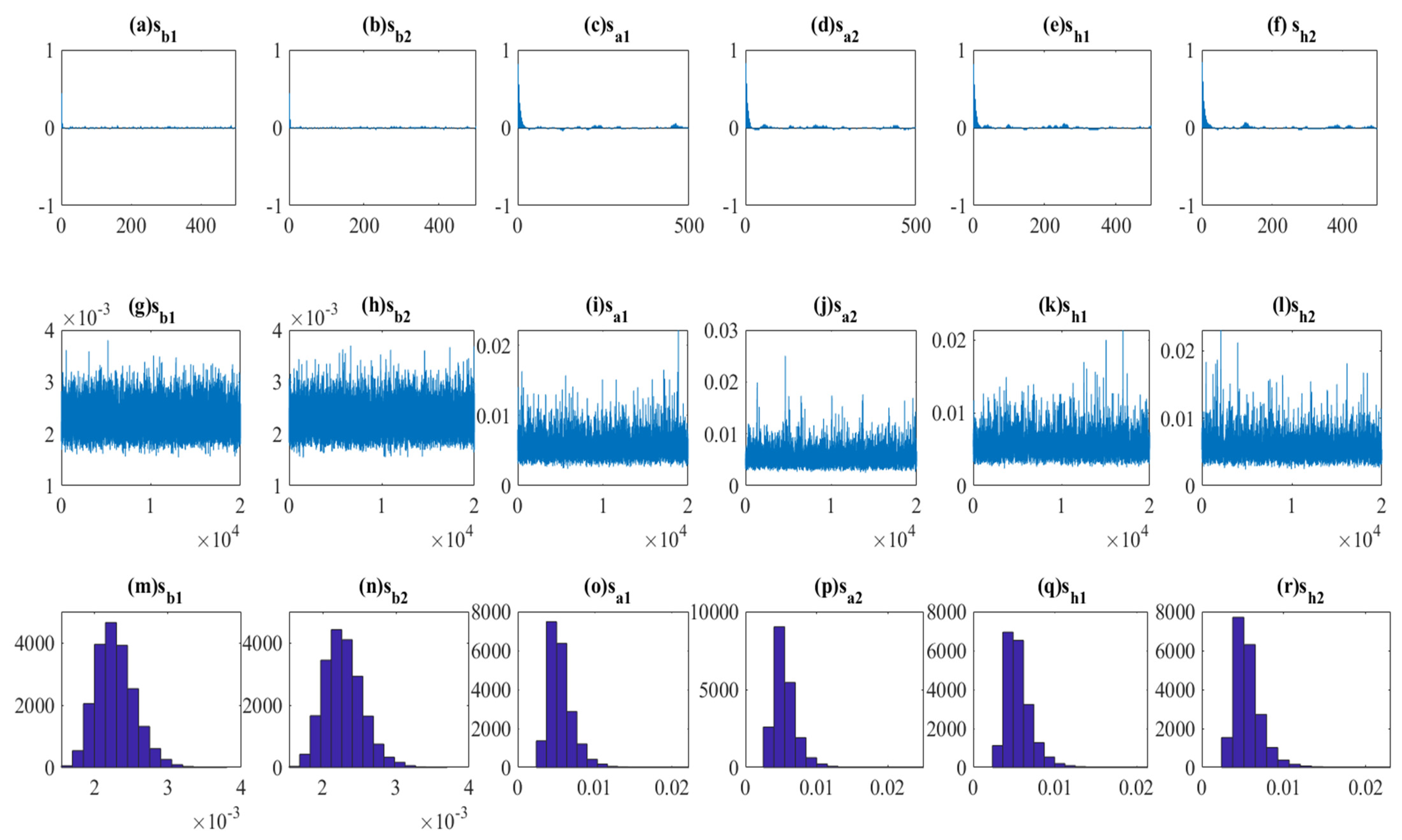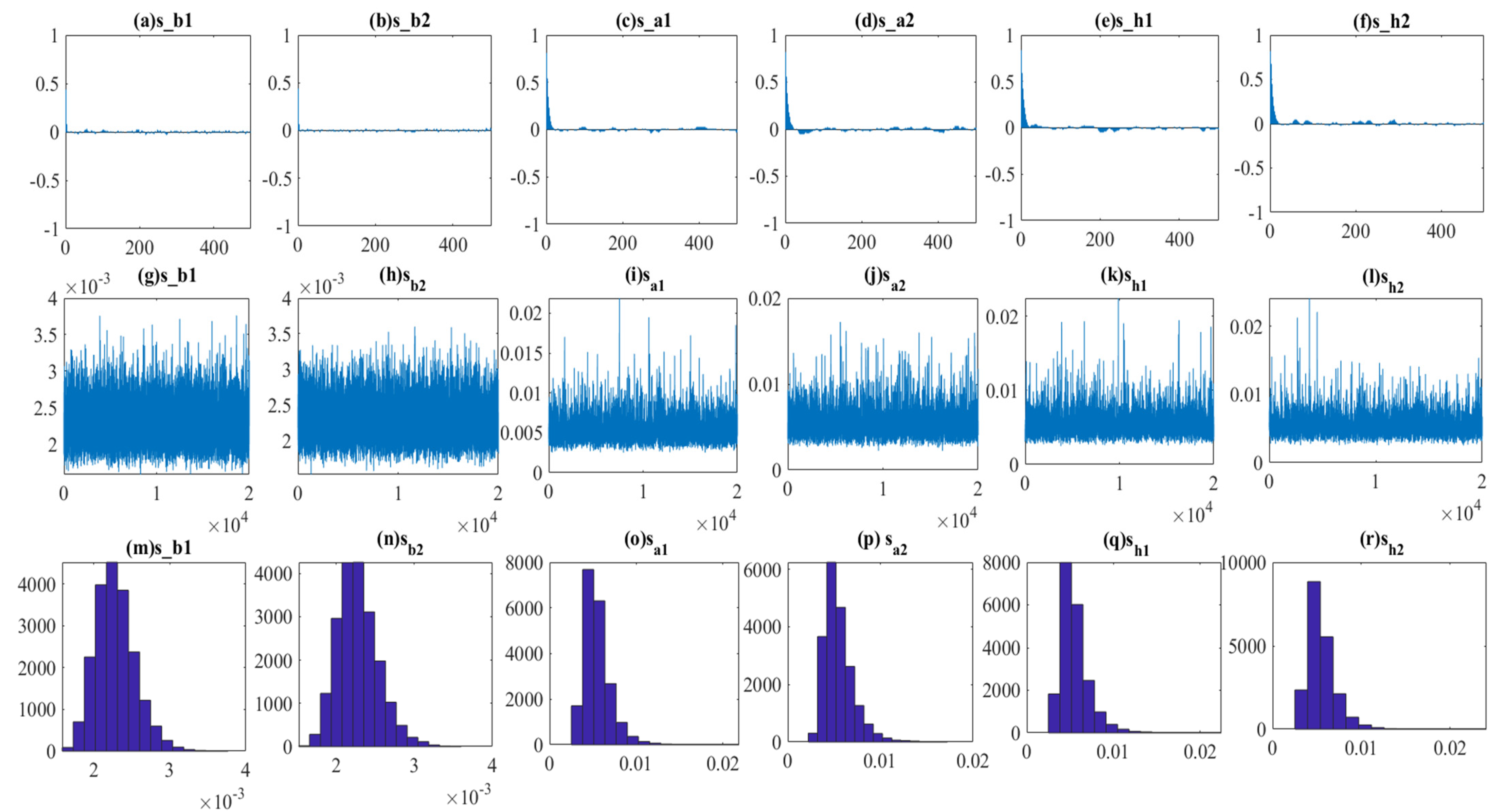Figure A1 and Figure A2 show the sample autocorrelation function, the sample paths, and the posterior densities for the selected parameters. After discarding the initial 2000 samples in the burn-in period, the sample paths look stable, and the sample autocorrelations drop smoothly.

Table 5. Markov-switching dynamic regression for gross domestic product.

Economic Variables	Estimations
	1	2	3	4
	$\mathit{G}\mathit{D}\mathit{P}$	$\mathit{G}\mathit{D}\mathit{P}$	$\mathit{G}\mathit{D}\mathit{P}$	$\mathit{G}\mathit{D}\mathit{P}$
State 1
$AOLR$		0.316 ***	1.255 ***	0.518 ***
		(3.55)	(15.99)	(6.94)
$AKLR$		−0.888 ***	−1.107 ***	−0.593 ***
		(−15.73)	(−24.51)	(−16.56)
$CPI$		1.773 ***	−0.0401	0.0855
		(7.34)	(−0.73)	(1.17)
$M3$			−0.169 ***	−0.708 ***
			(−5.79)	(−13.19)
$IR$				0.592 ***
				(9.65)
$\_cons$	−2.003 *	−6.924 ***	3.102 ***	1.359 ***
	(−2.64)	(−6.44)	(10.16)	(6.36)
State 2
$AOLR$		1.015 ***	0.927 ***	0.998 ***
		(31.91)	(24.69)	(43.19)
$AKLR$		−0.230 ***	−0.213 ***	−0.202 ***
		(−8.29)	(−8.70)	(−10.60)
$CPI$		0.0486 *	0.0104	−0.00610
		(2.45)	(0.45)	(−0.52)
$M3$			0.0399 ***	0.00901
			(4.62)	(1.24)
$IR$				0.0432 **
				(3.00)
$\_cons$	2.757 ***	1.313 ***	1.148 ***	1.131 ***
	(6.91)	(7.96)	(6.67)	(9.64)
N	32	32	32	32

t statistics in parentheses; * p < 0.05, ** p < 0.01, *** p < 0.001.

reflects the Markov chain dynamic regression model for the gross domestic product from 1990 to 2021. The result is of interest to the estimation of the impact of money supply on economic growth in different states. In state 1, estimation 1, $GDP$ is found to have a negative gross domestic product state mean2 rate of 2.00%, which is statistically significant at a 5% p-value. In estimation 4, it is found that a 1% increase in $M3$ results in a 0.70% fall in $GDP$ holding all other factors constant, and it is statistically significant at a 5% p-value. This implies that $M3$ in state 1 does not predict any positive effect on economic growth. The result is consistent with the theoretical assertion of Monetarists who assumed that money supply affects the price level, not the real GDP or unemployment level. South Africa cannot afford to be in this state of the economy, as it may not be able to fight other macroeconomic challenges of poverty, inequality, and unemployment. Moreover, this state of the economy will reflect that South Africa is far off in achieving the objective of the NDP of having an economic growth rate of 5%. Given that in this state there is negative growth output, an increase in the money supply may be detrimental as it can lead to much money chasing few goods. In a event of an increase in the price level. This would not be good for the general public as the wage sticks; therefore, the real wage will fall and affect aggregate consumption and the fall in the gross domestic product. In this, the increase in the money supply may have several negative multiplier effects. In state 2, estimation 1 of $GDP$ is found to have a positive mean of 2.75%, which is statistically significant at a 1% p-value. In estimation 4, it is found that $M3$ is statistically insignificant at a 5% p-value. This is in line with Keynesians’ view that the money supply has a limited influence on economic growth. However, when the monetary policy instrument of $IR$ is not factored in, it is found that there is a 1% increase in $M3,$ and estimation 3 is found to increase $GDP$ by 0.03%. This result suggests that in a positive economic growth state with less monetary policy through the interest rate, money may have a positive spillover on economic growth. These results are similar to those found by Denbel et al. (2016).

Table 6. Markov-switching dynamic regression for inflation.

Economic Variables	Estimations
	1	2	3	4
	$\mathit{C}\mathit{P}\mathit{I}$	$\mathit{C}\mathit{P}\mathit{I}$	$\mathit{C}\mathit{P}\mathit{I}$	$\mathit{C}\mathit{P}\mathit{I}$
State 1
$M3$		0.160	0.0238 ***	−0.0576 ***
		(1.45)	(0.17)	(−0.70)
$GDP$		0.672 ***	0.283	0.600 ***
		(4.88)	(1.32)	(4.17)
$IR$			−0.844 ***	−0.589 ***
			(−3.98)	(−3.41)
$ORE$			−0.822	−0.536
			(−1.34)	(−1.47)
$FIR$				−0.204
				(−1.65)
$\_cons$	5.703 ***	−4.498	16.06 ***	10.14 **
	(11.97)	(−1.89)	(4.47)	(3.03)
State 2
$M3$		−0.0699	0.245 ***	0.358 ***
		(−0.75)	(1.26)	(3.43)
$GDP$		0.914 ***	0.403	−0.0770
		(8.36)	(0.96)	(−0.45)
$IR$			0.222	0.239
			(1.05)	(1.82)
$ORE$			−1.141 *	−1.139 ***
			(−2.39)	(−3.73)
$FIR$				−0.697 **
				(−2.95)
$\_cons$	13.24 ***	0.0977	−0.323	3.512 **
	(6.66)	(0.12)	(−0.14)	(2.91)
N	32	32	32	32

t statistics in parentheses; * p < 0.05, ** p < 0.01, *** p < 0.001.

reflects the Markov chain dynamic regression model from 1990 to 2021. The results are of interest to the estimation of the impact of money supply on inflation in different states. In state 1, estimation 1 of $CPI$ is found to have a mean of 5.70%, which is statistically significant at a 1% p-value. In estimation 4, it is found that a 1% increase in $M3$ results in a 0.05% fall in $CPI$ holding all other factors constant, and it is statistically significant at a 5% p-value. These results are similar to those of Sean (2019), who found that the money supply induces an inflation rate of 0.13%. State 1 inflation means is within the target of 3% to 6%, and the result implies that the monetary tool of the money supply is effective in stabilising prices when inflation is within range. In state 2, estimation 1 of $CPI$ is found to have a mean of 13.24%, which is statistically significant at a 1% p-value. In estimation 4, it is found that a 1% increase in $M3$ results in a 0.35% increase in $CPI$ holding all other factors constant, and it is statistically significant at a 1% p-value. This result suggests that the monetary instrument of the money supply is not effective in reducing the price level when the inflation rate is above the range of 3% to 6%.

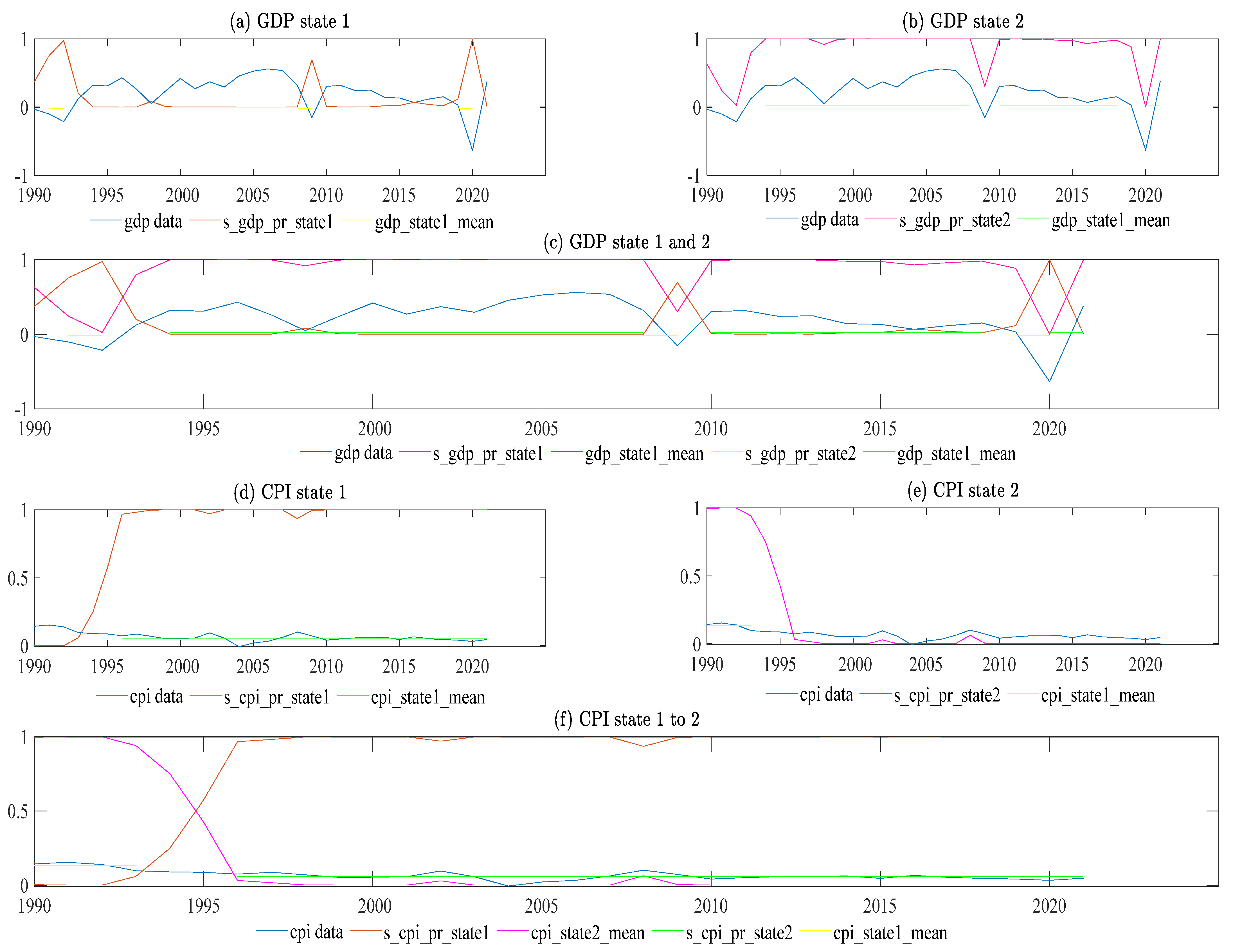
Figure 1 reflects state 1 to 2 filter transition probabilities and the data of $GDP$ and $CPI$. Figure 1 graph a reflects the filter transition probabilities for state 1 for $GDP$, which is characterised by a negative mean of 2.00%. The $GDP$ is found to move to state one in two episodes, first in 1994 and second in 2019. This reflects that most of the time, South African economic growth is not prone to stay in a negative state. As such, the result reflects that the economy may recover faster in the occurrence of a recession. Figure 1 graph b reflects the filter transition probabilities for state 2, which is characterised by a negative mean of 2.84%. It is found that the economy moved to this state three times. The economy was in state 2 from 1994 to 2008. The economy moved back to this state from 2010 to 2018, and the last move to this state was in 2021. Figure 1 graph c reflects states 1 to 2 for $GDP$ moving from state to state over time. Figure 1 graph d reflects the filter transition probabilities for state 1 for $CPI$, which is characterised by a mean of 5.70%. $CPI$ is found to move to state one from 1996 to 2021. Figure 1 graph e reflects the filter transition probabilities for state 2, which is characterised by a negative mean of 13.24%. The economy moved to this state in 1993. Figure 1 graph f reflects states 1 to 2 for $CPI$ moving from state to state over time.

Table 7. Transition probabilities.

$\mathbf{Estimate}\mathbf{for}\mathit{G}\mathit{D}\mathit{P}$				$\mathbf{Estimate}\mathbf{for}\mathit{C}\mathit{P}\mathit{I}$
Transition Probabilities				Transition Probabilities
$p_{11}$	0.9162037	$p_{12}$	0.0837963	$p_{11}$	0.8492753	$p_{12}$	0.1507247
$p_{21}$	0.0615749	$p_{22}$	0.9384251	$p_{21}$	0.1985816	$p_{22}$	0.8014184
Number of obs = 31				Number of obs = 31

shows the transition probabilities of the two states for both $GDP$ and $CPI$. There is a 91% chance that $GDP$ will move from state one and return to state one. However, there is a 93% chance that $GDP$ will move from state two and return to state two. For $CPI$, there is an 84% chance that $CPI$ will move from state one and return to state one. There is evidence that there is an 80% chance that $CPI$ will move from state two and return to state two.

Table 8. Expected duration.

Estimate for $\mathit{G}\mathit{D}\mathit{P}$		Estimate for $\mathit{C}\mathit{P}\mathit{I}$
States	Expected Duration	States	Expected Duration
State 1	11.93371	State 1	6.634613
State 2	16.24039	State 2	5.035713
Number of obs = 31		Number of obs = 31

reflects the expected duration to be spent in each state. It is found that $GDP$ will be in state 1 for 11 years and spend 16 years in state 2. On the other hand, $CPI$ is expected to be in state 1 for 6 years and 5 years in state 2.

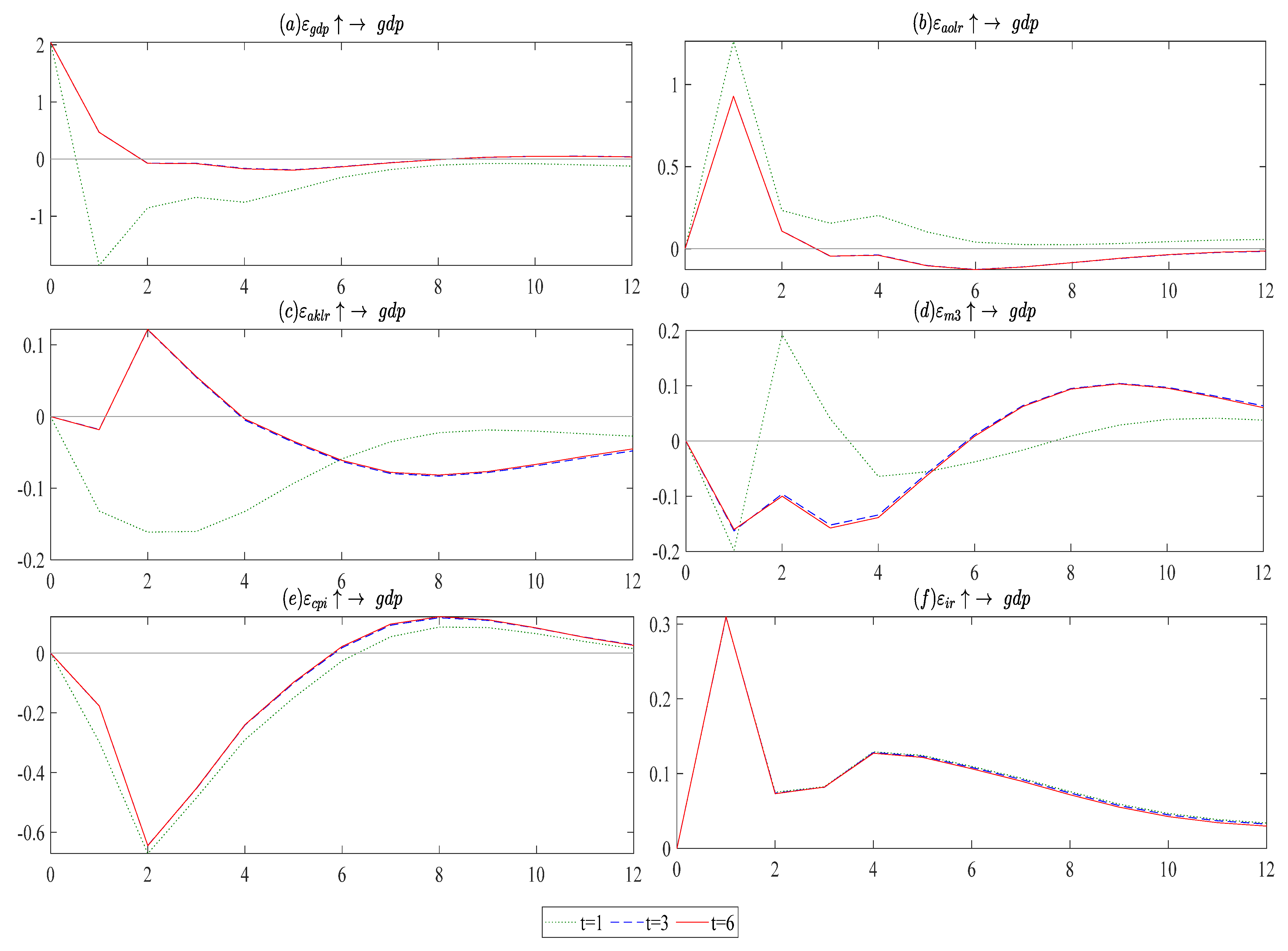
Figure 2 shows the time-varying posterior of impulse response shocks to gross domestic product. In Figure 2, graph d, there is a reflection of the shock ${\epsilon }_{M3}\uparrow \to GDP$ of $M3$ to $GDP$. It is found that $M3$ shock results in a fall in the $GDP$ in the first year by 0.15%. The $GDP$ after that starts becomes to be cyclical with the increase rate to 1% and thereafter decreasing to 0.15%. In year 4 after the shock of $M3,$ $GDP$ begins to increase until it reaches equilibrium levels in year 6. Thereafter, $GDP$ operates above equilibrium with a maximum rate of 0.11%. Figure 2, graph e, shows the impact of the shock ${\epsilon }_{CPI}\uparrow \to GDP$ of $CPI$ on $GDP$ reflects the decrease in the $GDP$ for two consecutive years with a negative rate of 0.1% and 0.6% in the respective first two years. The effect of high price levels in the economy state filters out as $GDP$ increases from year 2 to 6. However, a 2-year decrease in $GDP$ takes 4 years to recover after the shock of $CPI$. $GDP$ increases until it reaches a maximum of 0.2% in year 8 and thereafter moderates down to 0.1%. Figure 2, graph f, shows the shock ${\epsilon }_{IR}\uparrow \to GDP$ impact of $IR$ on $GDP$. The $IR$ reflects that there is a sharp increase in $GDP$ to 0.3%, which is a historical value recorded compared to other shocks in Figure 2. The sharp increase in year 1 is followed by a decrease in year 2, where $GDP$ reaches a rate of 0.9%. There is a downwards trend thereafter as the shock filters out. Nevertheless, the GDP still operates above equilibrium.

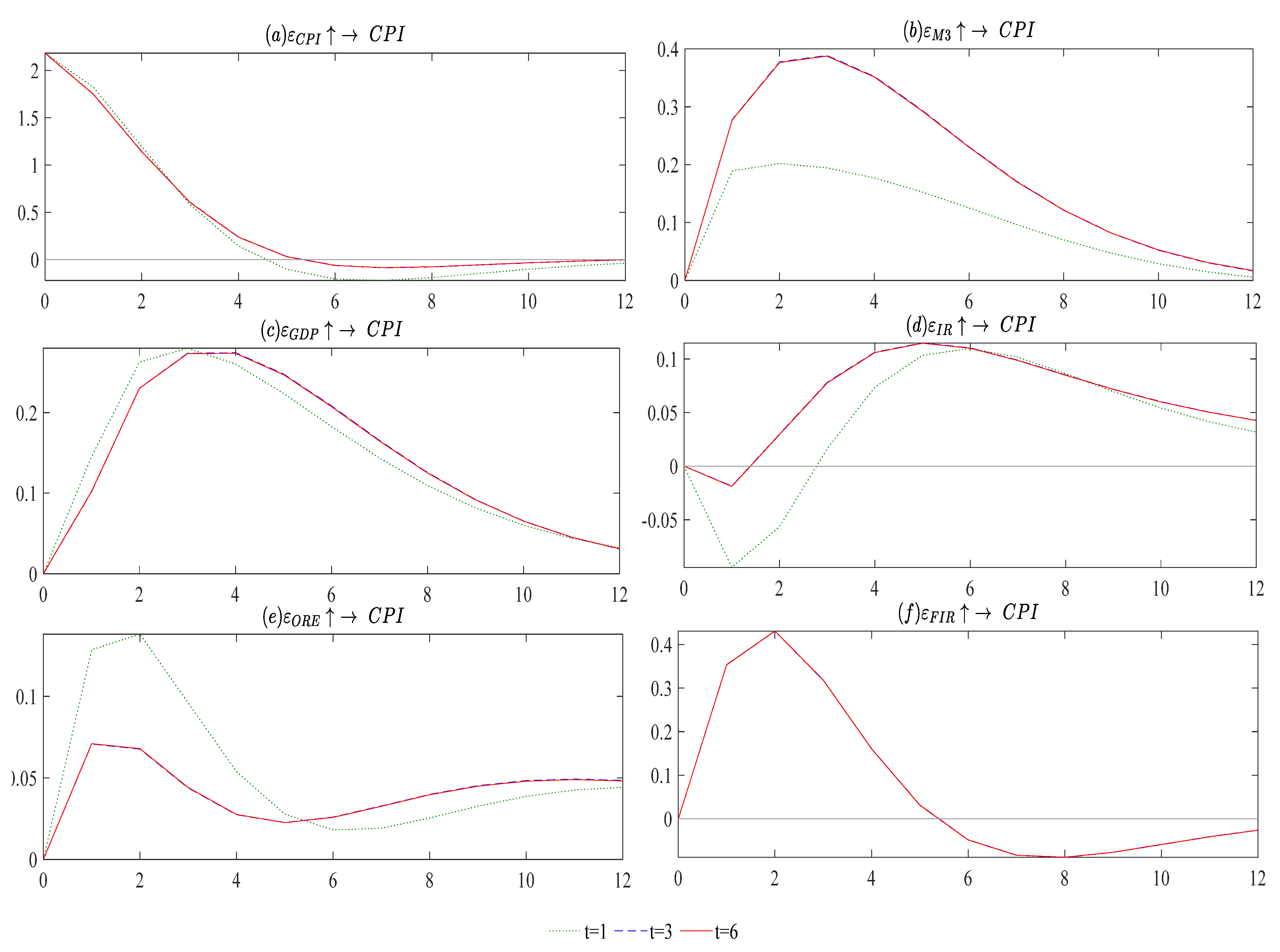
Figure 3 shows the time-varying posterior of impulse response shocks to inflation. Figure 3, graph b, shows the shock ${\epsilon }_{M3}\uparrow \to CPI$ of $M3$ to $CPI$. It is found that $M3$ shock results in an increase in the $CPI$ which is increasing at a decreasing rate up until it reaches the maximum of 0.39%. Thereafter, the shock filters out in year 12, which shows that it takes 9 years for the shock to filter out in the economic system. Figure 3, graph c, shows the shock ${\epsilon }_{GDP}\uparrow \to CPI$ of $GDP$ to $CPI$. The result of the $GDP$ shock to $CPI$ is similar to the $M3$ shock to $CPI$ with the difference in the magnitude, as the $GDP$ results in an increase in $CPI$ by 0.29% at the maximum reached in year 4 after the shock. The shock of the $GDP$ after year 4 starts to filter out. However, the inflation rate operates above equilibrium. This reflects that there is no full recovery from high price levels when there is a positive shock in $GDP$. Figure 3, graph c, shows the shock ${\epsilon }_{IR}\uparrow \to CPI$ of $IR$ to $CPI$. The $IR$ is one of the conventional monetary policy instruments. The positive shocks of $IR$ result in the desired result of a decrease in inflation. However, this decrease is marginal, with a rate of 0.03% in year 1 after the shock. Thereafter, inflation starts to increase until it reaches a maximum of 0.13% in year 5. After the maximum is reached, inflation moderates but operates above equilibrium.

5. Conclusions

This paper investigates the impact of the money supply on inflation and economic growth in South Africa from 1990 to 2021. The paper acknowledges that there are no censuses on the empirical and theoretical levels of the impact of money supply, inflation, and economic growth. The economic variable of interest, economic growth, is pretesting below the target of 5%, as is the National Development Plan, and the mean of the study period is 2.06%. On the other hand, inflation has reflected floatation, and in recent times, it has been in the high band of 6%. On the other hand, the rand value of the money supply, which is part of unconventional monetary policy, has increased over the years. The key economic question of this paper is as follows: what is the impact of money supply on economic growth and inflation in a different state? Therefore, the sub-questions are as follows: What is the probability of economic growth and inflation moving from state to state? How long will economic growth and inflation be in a state? What is the time-varying elasticity impact of money supply on economic growth and inflation in different states? What is the impact of money shocks on economic growth and inflation?

The theoretical framework of Cobb–Douglas was used to investigate the impact of the money supply on economic growth. On the other hand, the classical quantity theory of money was used to investigate the impact of the money supply on inflation. Markov-switching dynamic regression (MSDRM) and time-varying parameter structural vector autoregression (TVP-VAR) were adopted for estimation. There are two states for economic growth found, one with a negative rate of 2.00% and the other with a positive rate of 2.75%. There is a 91% and 93% chance that the economy can move and return to the same state both in states one and two. Currently, South Africa is in a positive state, which increases optimism that the money supply can further be used as an instrument to increase economic growth to meet the macroeconomic objectives outlined in the NDP to achieve 5% economic growth. However, given the high chance of staying in a negative state as well, the money supply has a negative impact on economic growth. This reflects that South Africa’s economy is fragile, and monetary tools may not be accommodative in the effort to restore aggregate demand. In such an event, South Africa will likely have a recession and monetary policy may not be fully effective in assisting the economy in recovery.

Similarly, inflation is found to have two states characterised by a mean rate of 5.70% and 13.24% with 84% and 80% changes in moving and returning to states 1 and 2, respectively. State one is better since it reflects a mean that is within the range of the inflation target of 3% to 6%. Moreover, the money supply is found to reduce inflation, which reflects the effectiveness of monetary policy in reducing inflation. Based on the results, monetary policy should be planned to maintain price stability by controlling the growth of the money supply in the economy. State two reflects the time when the SARB was not under inflation targeting. If the economy reaches this state the money supply is not effective in reducing inflation, as it results in a 0.35% increase in the inflation rate.

Money supply has a prime impact on economic growth, and money supply shocks are found to have a negative impact on gross domestic product. However, the money eventually moves economic growth above equilibrium in year 8. This, therefore, implies that monetary policy instruments play an important role in output growth and other macroeconomic policies in the long run. As such, it is recommended that the money supply be used for the long-run plan rather than the short-run plan. The estimated money supply reflected that there would be an increase in the inflation rate. Therefore, it implies that monetary expansion has continued as the key contributing factor to the persistent increase in the price level in South Africa. The stability of the overall price level will be impacted by the money supply; thus, South African monetary authorities need to exert stronger control over it. This will assist in avoiding inflation by moving to the economic state that is 2 times above the higher band inflation target.

References

1. Adu, George, and George Marbuah. 2011. Determinants of Inflation In Ghana: An Empirical Investigation. South African Journal of Economics 79: 251–69. [Google Scholar] [CrossRef]
2. Al-Mutairi, Abdullah, Sulaiman Al-Abduljader, and Kamal Naser. 2020. Determinants of inflation in Kuwait. Journal of Developing Areas 54: 19–34. [Google Scholar] [CrossRef]
3. Amassoma, Ditimi, Keji Sunday, and Emma-Ebere Onyedikachi. 2018. The influence of money supply on inflation in Nigeria. Journal of Economics & Management 31: 5–23. [Google Scholar]
4. Amisano, Gianni, and Gabriel Fagan. 2010. Money growth and inflation: A regime switching approach. European Central Bank, Working Paper Series 33: 118–45. [Google Scholar] [CrossRef]
5. Aslam, Ahamed Lebbe Mohamed. 2016. Impact of money supply on Sri Lankan economy: An econometric analysis. International Letters of Social and Humanistic Sciences 67: 11–17. [Google Scholar] [CrossRef]
6. Azam, Muhammad, and Saleem Khan. 2022. Threshold effects in the relationship between inflation and economic growth: Further empirical evidence from the developed and developing world. International Journal of Finance & Economics 27: 4224–43. [Google Scholar]
7. Bojanic, Antonio. 2021. A Markov-switching model of inflation in Bolivia. Economies 9: 37. [Google Scholar] [CrossRef]
8. Cesarano, Filippo. 2008. Monetary Systems and Monetary Theory. In Money and Monetary Systems. Cheltenham: Edward Elgar Publishing, pp. 79–95. [Google Scholar]
9. Chaitip, Prasert, Kanchana Chokethaworn, Chukiat Chaiboonsri, and Monekeo Khounkhalax. 2015. Money supply influencing on economic growth-wide phenomena of AEC open region. Procedia Economics and Finance 24: 108–15. [Google Scholar] [CrossRef]
10. Danlami, Ibrahim Abdulhamid, Mohamad Helmi Hidthiir, and Sallahuddin Hassan. 2020. Money supply and inflation in Nigeria: The myth of the monetarist theory of inflation. Journal of Economics and Sustainability 2: 1–13. [Google Scholar] [CrossRef]
11. Denbel, Fitsum Sharew, Yilkal Wassie Ayen, and Teshome Adugna Regasa. 2016. The relationship between inflation, money supply and economic growth in Ethiopia: Cointegration and Causality Analysis. International Journal of Scientific and Research Publications 6: 556–65. [Google Scholar]
12. Dingela, Siyasanga, and Hlalefang Khobai. 2017. Dynamic impact of money supply on economic growth in South Africa. An ARDL Approach 2: 2–18. [Google Scholar]
13. Doan Van, Dinh. 2019. Money supply and inflation impact on economic growth. Journal of Financial Economic Policy 12: 121–36. [Google Scholar] [CrossRef]
14. du Rand, Gideon, Ruan Erasmus, Hylton Hollander, Monique Reid, and Dawie van Lill. 2021. The evolution of central bank communication as experienced by the South Africa Reserve Bank. Economic History of Developing Regions 36: 282–312. [Google Scholar] [CrossRef]
15. Emmanuel, Udo, Ben Etim Udoh, Abner Ishaku Prince, Johnson Okoh, and Okolo Marvis Ndu. 2019. Money supply and inflation rate in Nigeria: The missing link. Humanities 7: 156–66. [Google Scholar]
16. Fed-USA. 2022. Fed Economics Data: M3 for South Africa, National Currency, Annual, Seasonally Adjusted (MABMM301ZAQ657S). Available online: https://fred.stlouisfed.org/series/MABMM301ZAQ657S (accessed on 11 November 2022).
17. Friedman, Milton. 1989. Quantity theory of money. In Money. Berlin/Heidelberg: Springer, pp. 1–40. [Google Scholar]
18. Geweke, J. 1992. Evaluating the accuracy of sampling-based approaches to the calculations of posterior moments. Bayesian Statistics 4: 641–49. [Google Scholar]
19. Hamilton, James D. 1989. A new approach to the economic analysis of nonstationary time series and the business cycle. Econometrica: Journal of the Econometric Society 40: 357–84. [Google Scholar] [CrossRef]
20. Hamilton, James D. 1990. Analysis of time series subject to changes in regime. Journal of Econometrics 45: 39–70. [Google Scholar] [CrossRef]
21. Hansen, Bruce E. 1996. Inference when a nuisance parameter is not identified under the null hypothesis. Econometrica: Journal of the Econometric Society 64: 413–30. [Google Scholar] [CrossRef]
22. Hansen, Bruce E. 2000. Sample splitting and threshold estimation. Econometrica 68: 575–603. [Google Scholar] [CrossRef]
23. Hollander, Hylton, and Dawie Van Lill. 2019. A Review of the South African Reserve Bank’s Financial Stability Policies. Stellenbosch: Stellenbosch University, Department of Economics. [Google Scholar]
24. Hossain, Akhand Akhtar, and Popkarn Arwatchanakarn. 2017. Does Money Have a Role in Monetary Policy for Price Stability under Inflation Targeting in Thailand? Journal of Asian Economics 53: 37–55. [Google Scholar] [CrossRef]
25. Hussain, Muhammad Ijaz, and Tasneem Zafar. 2018. The interrelationship between money supply, inflation, public expenditure and economic growth. European Online Journal of Natural and Social Sciences 7: 1–24. [Google Scholar]
26. Ilyas, Muhammad, Liying Song, Mukhtar Danladi Galadima, Muhammad Noshab Hussain, and Abdul Sattar. 2022. Shocks effects of inflation, money supply, and exchange rate on the West African Monetary Zone (WAMZ): Asymmetric SVAR modelling. The Journal of International Trade & Economic Development 31: 255–76. [Google Scholar]
27. Inam, Uduakobong S., and Blessing Sunday Ime. 2017. Monetary policy and economic growth in Nigeria: Evidence from Nigeria. Advances in Social Sciences Research Journal 4: 150–84. [Google Scholar] [CrossRef]
28. Inim, Victor, Udo Emmanuel Samuel, and Abner Ishaku Prince. 2020. Other determinants of inflation in Nigeria. European Journal of Sustainable Development 9: 338–38. [Google Scholar] [CrossRef]
29. Koop, Gary, and Dimitris Korobilis. 2018. Variational Bayes Inference in High-Dimensional Time-Varying Parameter Models. Colchester: University of Essex, Essex Business School. [Google Scholar]
30. Madito, Oatlhotse, and Nicholas M. Odhiambo. 2018. The main determinants of inflation in South Africa: An empirical investigation. Organizations and Markets in Emerging Economies 9: 212–32. [Google Scholar] [CrossRef]
31. Mankiw, N. Gregory. 2014. Principles of Economics. Belmont: Cengage Learning. [Google Scholar]
32. Maune, Alexander, Ephraim Matanda, and Justice Mundonde. 2020. Is Money Supply the Cause of Inflation in Zimbabwe? An Empirical Examination. Acta Universitatis Danubius. OEconomica 16: 17–37. [Google Scholar]
33. Meyer, Daniel Francois, Jacques De Jongh, and Devan Van Wyngaard. 2018. An assessment of the effectiveness of monetary policy in South Africa. Acta Universitatis Danubius. OEconomica 14: 281–95. [Google Scholar]
34. Monamodi, Nkosinathi. 2019. The impact of fiscal and monetary policy on economic growth in Southern African Custom Union (SACU) member economies between 1980 and 2017: A panel ARDL approach. Monetary and Economic Studies 15: 86–102. [Google Scholar] [CrossRef]
35. Mpofu, Raphael T. 2011. Money supply, interest rate, exchange rate and oil price influence inflation in South Africa. Corporate Ownership and Control 8: 594–605. [Google Scholar] [CrossRef]
36. Nakajima, Jouchi. 2011. Time-varying parameter VAR model with stochastic volatility: An overview of methodology and empirical applications. Monetary and Economic Studies 29: 107–42. [Google Scholar]
37. Obi, Kenneth O, and Anthony Ajana Uzodigwe. 2015. Dynamic Impact of Money Supply on Inflation: Evidence from ECOWAS Member States. Journal of Economics and Finance (IOSR-JEF) 6: 10–37. [Google Scholar]
38. Ofori, Collins Frimpong, Benjamin Adjei Danquah, and Xuegong Zhang. 2017. The impact of money supply on inflation, a case of Ghana. Imperial Journal of Interdisciplinary Research 3: 2312–18. [Google Scholar]
39. Ozekhome, Hassan O. 2017. Does money supply growth cause inflation in the West African Monetary Zone? West African Journal of Monetary and Economic Integration, West African Monetary Institute 17: 57–80. [Google Scholar]
40. Phiri, Andrew. 2018. Nonlinear impact of inflation on economic growth in South Africa: A smooth transition regression analysis. International Journal of Sustainable Economy 10: 1–17. [Google Scholar] [CrossRef]
41. Precious, Chipote, and Palesa Makhetha-Kosi. 2014. Impact of monetary policy on economic growth: A case study of South Africa. Mediterranean Journal of Social Sciences 5: 76. [Google Scholar] [CrossRef]
42. Primiceri, Giorgio E. 2005. Time-varying structural vector autoregressions and monetary policy. The Review of Economic Studies 72: 821–52. [Google Scholar] [CrossRef]
43. Runde, Jochen. 1994. Keynesian uncertainty and liquidity preference. Cambridge Journal of Economics 18: 129–44. [Google Scholar]
44. Sabade, Shubhada. 2014. Is Money Supply the Cause of Inflation in India? An Alternative Postulate to Understand Inflation. Procedia—Social and Behavioral Sciences 133: 379–82. [Google Scholar] [CrossRef]
45. SARB. 2022. Online Statistical Query (Historical Macroeconomic Timeseries Information). Available online: https://www.resbank.co.za/Research/Statistics/Pages/OnlineDownloadFacility.aspx (accessed on 11 November 2022).
46. Sean, Monorith. 2019. The Impact of Monetary Policy on Economic Growth in Cambodia: Bayesian Approach. Journal of Management, Economics, and Industrial Organization 3: 16–34. [Google Scholar] [CrossRef]
47. Sims, Christopher A. 1980. Martingale-Like Behavior of Prices. Cambridge: National Bureau of Economic Research. [Google Scholar]
48. Tegegne, Yeshiwas Ewinetu. 2021. Impact of Broad Money Supply on Economic Growth of Ethiopia. Research Journal of Finance and Accounting 12: 20–45. [Google Scholar]
49. World-Bank. 2022. DataBankWorld Development Indicators. Available online: https://databank.worldbank.org/indicator/NY.GDP.MKTP.KD.ZG/1ff4a498/Popular-Indicators (accessed on 11 November 2022).
Figure 1. Transition probability to different states for GDP and CPI. Note: G D P is the gross domestic product, C P I is the inflation rate, S _ C P I _ s t a t e 1 , S _ C P I _ s t a t e 2 , S _ G D P _ s t a t e 1 , and S _ G D P _ s t a t e 2 reflect different states, and G D P _ m e a n and CPI _ m e a n reflect the average mean of GDP and CPI in the period of investigation. The state mean reflects the average of that economic variable interest when it is in that particular state. A state will run for a specific period; therefore, the model can generate the mean or average.
Economies 11 00064 g001
Figure 2. Time-varying posterior of impulse responses shocks to gross domestic product. Note the description for c p i is the inflation rate, m 3 money growth rate (money supply), a o l r average output labour ratio, a o k r average output capital ratio, g d p economic growth rate, and i r nominal interest rate.
Economies 11 00064 g002
Figure 3. Time-varying posterior of impulse responses shocks to inflation. Note the description for c p i is the inflation rate, m 3 money growth rate (money supply), g d p economic growth rate, i r nominal interest rate, o r e exchange rate, f i r foregine interest rate and i r nominal interest rate.
Economies 11 00064 g003