1. Introduction
“We tend to use [transitory] to mean that it won’t leave a permanent mark in the form of higher inflation. I think it’s probably a good time to retire that word and try to explain more clearly what we mean”, Federal Reserve Chairman Jerome Powell said during a congressional hearing on Tuesday, 2 December 2021.
To combat the negative economic effects of COVID-19, the Federal Reserve has used an unprecedented combination of monetary and fiscal policies.
Clarida et al. (
2021) provides an excellent summary of how the Federal Reserve deployed its conventional tools to support the U.S. economy in 2020 and contribute to robust economic recovery in 2021. The tools included large-scale asset purchase programs (
Vissing-Jorgensen 2021), near-zero interest rates, and subsidized loan programs. On top of the expansionary monetary policies, Congress authorized various types of expansionary fiscal policies, including the
$2.2 trillion Coronavirus Aid, Relief, and Economic Security (CARES) Act (
Bhutta et al. 2020).
These expansionary monetary and fiscal policies led to a large increase in the supply of money.
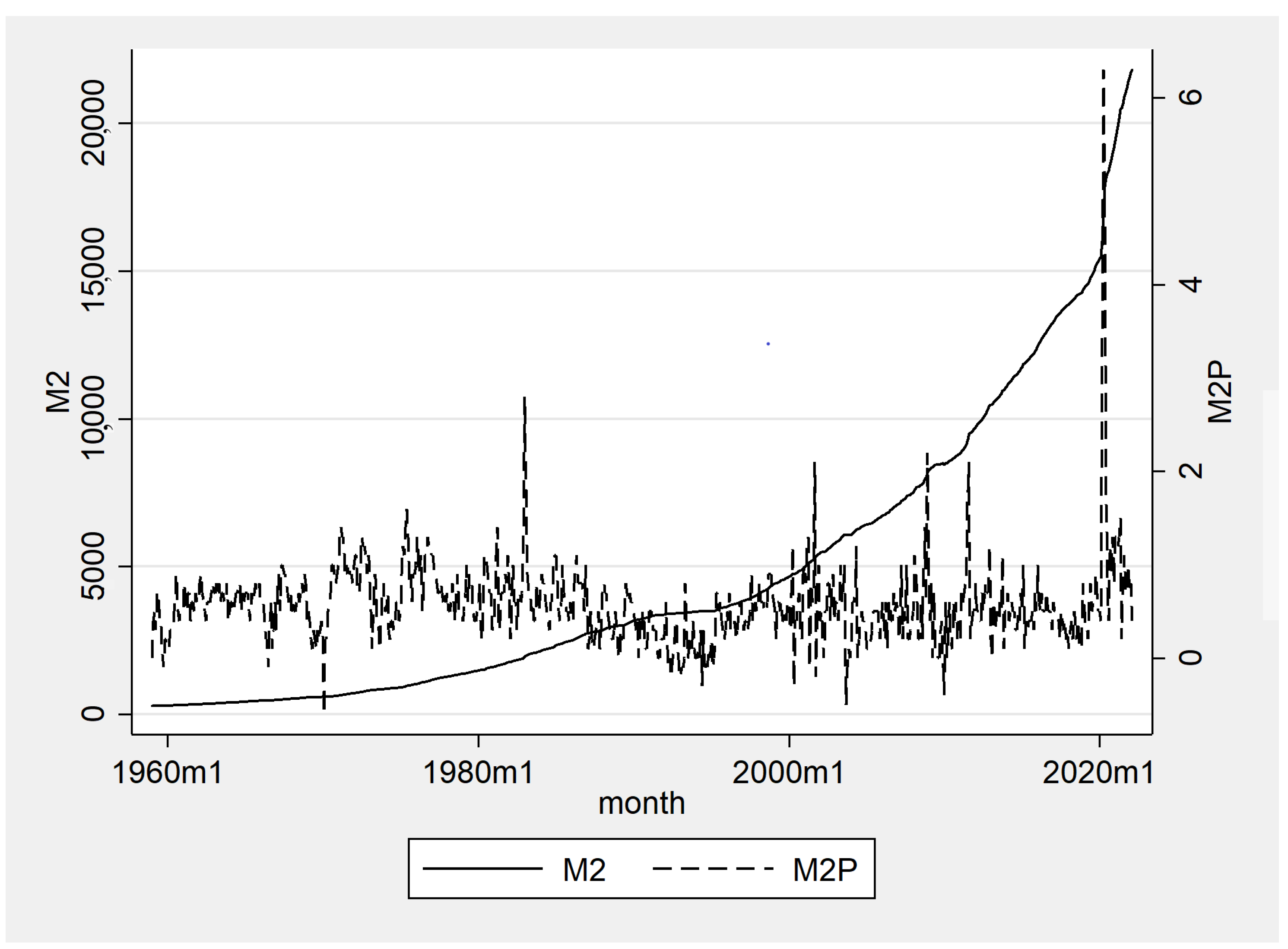
Figure 1 depicts M2 money supply (M2) in seasonally adjusted billions of dollars and its percent change (M2P) at a monthly level from 1959:01 to 2022:02. M2 since 1959 shows a slow and steady growth until 2000, growing to approximately
$5 trillion in the 40-year span. Between 2000 and 2020, M2 grew from
$5 trillion to
$15 trillion, an increase of
$10 trillion in 20 years. Due to the aforementioned expansionary policies in response to COVID-19, the level of M2 grew from approximately
$15 trillion in 2020:01 to
$22 trillion in 2022:02, an increase of
$7 trillion in 2 years. The magnitude of the increase in M2 is quite astonishing compared to the rather slow and steady historical growth. At any month since 1959 and before 2020, the monthly percent change in M2 was within 2 percent except for 2.8 percent in 1983:01, which occurred during the oil shock crisis. Even during the Global Financial Crisis of 2007–2009, the monthly growth rate was within the 2 percent range. In contrast, the COVID-19 money supply growth rate is unprecedented. In March, April, and May 2020, the money supply grew by 3.4, 6.3, and 4.9 percent, respectively.
With the increase in the money supply, the debate about its impact on inflation has reemerged. The original idea behind the relationship between the money supply and inflation stems from the quantity theory of money (
Humphrey 1974). The theory states that the quantity of money in circulation primarily affected the general level of prices.
Brunner and Meltzer (
1972);
Brunner et al. (
1980);
Cagan (
1989);
Friedman (
1989);
Friedman and Schwartz (
2008), and other monetarists show that a sudden increase in the money supply resulted in a proportional increase in inflation, and hence, the government should curtail the money supply to control the price level. In contrast,
Ball et al. (
1988);
Cogley and Sbordone (
2008);
Del Negro et al. (
2015);
Galí (
2015), and other Keynesian economists have challenged the quantity theory of money. The main argument is that an increase in the money supply has led to a decrease in the velocity of money and a rise in real income, which would stimulate aggregate demand and the economy would achieve full employment. For instance,
Mishkin (
2009) contends that the expansionary monetary policy was effective in reducing adverse effects from financial disruptions and managing an upward shift in inflation risks during the Global Financial Crisis.
However, the price level in the U.S. has substantially been increasing since 2021 and well into 2022. At the end of 2021, Federal Reserve Chairman Jerome Powell acknowledged that the upward trend in inflation is no longer transitory, reversing from the original stance.
1 The headline U.S. inflation rate rose to 7.5 percent in January 2022, which is the highest rate of increase since 1982.
2 The core personal consumption expenditure (PCE) price index, the Federal Reserve’s preferred inflation gauge, rose to 5.2 percent, also with the highest rate of increase since 1983.
3 Given that the core PCE prices have been well over their target rate of 2 percent, the Federal Reserve increased the interest rate on March 2022, which is a major shift in the U.S. monetary policy, and it will continue to raise the rate at least until the end of 2022, although there is a disagreement about the incremental of each raise.
4Forecasting inflation after COVID-19 has been a difficult task using a traditional econometric model given the unique macroeconomic variations during the pandemic. Vector autoregression (VAR) is one of the most popular models in macroeconomics to measure the responses of outcome variables to exogenous shocks and forecast future outcomes (e.g.,
Giordano et al. 2007;
Gharehgozli et al. 2020). However, the COVID-19 pandemic has created challenges to the VAR model, as the U.S. economy experienced economic disruptions at an unprecedented scale. Namely, the unemployment rate in April 2020 was 14.7 percent, an increase of 10 percentage points in a single month.
Lenza and Primiceri (
2020) point out that this type of unprecedented irregularity in the data will contaminate the pre-pandemic fit of the VAR model.
To tackle the challenge of using a VAR model in times of a pandemic, macro-econometricians are trying to incorporate this outlier, extreme observation, or contamination of data into the model. The literature provides two major solutions. A first strand of literature applies restrictions to the estimation. For instance,
Lenza and Primiceri (
2020) suggest an ad hoc strategy of removing outliers for parameter estimation. Economists can re-scale the April 2020 parameter, provided that this re-scaling is common to all shocks. The solution provides a flexibility in the model because the exact timing of the volatility change is known, which makes it much simpler than a typical time-varying volatility model. Unfortunately, the proposed solution is not suitable for forecasting because it significantly undermines uncertainty.
Schorfheide and Song (
2021) suggest that an existing mixed-frequency VAR model can still be used with some modification without a major ad hoc change. However, the modification still includes excluding a few months of outliers, which could jeopardize the model’s forecasting performance. A second strand of literature gets help from additional information. For instance,
Foroni et al. (
2020) use information from the Global Financial Crisis to adjust post-pandemic forecasts.
Ng (
2021) treats COVID-19 as a persistent health crisis with large economic consequences and “de-COVID” the data so that economic shocks within the VAR model can be identified. COVID-19 indicators, such as hospitalization, positive cases, and deaths, are used to either eliminate or include additional information for the modeling.
In line with the literature proposing alternatives to the traditional VAR approach, we propose a new model to examine the macroeconomic behaviors in times of a pandemic. Our model stems from the point of view that macroeconomic outcomes that originate with labor market dislocations differ from those in which labor markets play a less active role. Namely, domestic lockdown policies across different U.S. states in March and April 2020 served as an exogenous shock to unemployment. The domestic lockdown policies are unprecedented even in past epidemic episodes, which make the COVID-19 recession unique compared to any other historical crises. Furthermore, the so-called “Great Resignation”, during which workers have voluntarily decided not to return to work until work safety and an increase in real wages are guaranteed, has increased instability in unemployment. Thus, we assume that the labor market has been substantially distorted during the pandemic due to exogenous shocks, such as the lockdown policies and the Great Resignation. Our logic is in sync with an argument made in
Aastveit et al. (
2017), which show that the association between GDP and unemployment has been shifted since the Global Financial Crisis in 2008.
The rest of this paper is structured as follows.
Section 2 presents our VAR model and describes the data.
Section 3 discusses findings from the main methodology and sensitivity analysis.
Section 4 concludes the paper.
2. Model Specification
In this section, we introduce our VAR model and the identification scheme for the structural shocks and then discuss our data.
A VAR model is, in principle, a simple multivariate model in which each variable is explained by its own past values and the past values of all the other variables. In other words, it describes the evolution of a set of k variables, called endogenous variables, over time and, therefore, enables us to study the responses of each variable to substantial changes in others through the impulse response analysis, forecast error variance decomposition, historical decomposition, and the analysis of forecast scenarios (e.g.,
Hashimzade and Thornton 2021).
In the econometrics literature, the main stimulus for much recent work on VAR models is the paper by
Sims (
1980), based on the idea of using an unrestricted vector of past values of variables for forecasting. Since then, the literature has been full of studies in which a VAR is employed to study the relationship between economic indicators, and many of these studies are focused on the dynamics of the macroeconomic variables and the effects of events and interventions on these dynamics (e.g.,
Adeniran et al. 2016;
Berisha 2020;
Okoro 2014;
Ronit and Divya 2014;
Zuhroh et al. 2018).
One advantage of the VAR model is that we can typically treat all variables as a priori endogenous. Thereby, they account for
Sims (
1980)’s critique that the exogeneity assumptions for some of the variables in simultaneous equations models are ad hoc and often not backed by fully developed theories (e.g.,
Hashimzade and Thornton 2021). A VAR model does not assume any direction for the relationships unless restricted. Restrictions, including the exogeneity of some of the variables, may be imposed on VAR models based on statistical procedures. Structural VAR analysis, then, attempts to investigate structural economic hypotheses with the help of VAR models. While in the structural VAR, variables can have contemporaneous effects on each other, in a reduced-form structural VAR, the contemporaneous effects are considered in the error term, and while no variable has a direct contemporaneous effect on other variables, the occurrence of one structural shock can potentially lead to the occurrence of shocks in all error terms, thus creating contemporaneous movement in all endogenous variables.
There are some caveats in working with the VAR models. The estimation of autoregressive models requires that the data be fully observed. With the existence of missing values, this is not possible, rendering it impossible to estimate the model (e.g.,
Bashir and Wei 2018), or large samples of observations involving time series variables that cover many years are needed to estimate the VAR model; these are seldom available for regional studies (e.g.,
LeSage and Krivelyova 1999). VAR models are criticized because they do not shed any light on the underlying structure of the economy, as they do not aim to estimate causal relationships. Though this criticism is not important when the purpose of VAR is forecasting, it is relevant when the objective is to find causal relations among the macroeconomic variables.
We find that the structural VAR explained below is an appropriate model to address the inquiry of this study, which is not necessary to estimate the causal relationships between the variables in the model, but to employ their dynamics to forecast the future of the main variable of interest. The structural VAR enables us to follow and include the observed structural pattern of the economy (after the pandemic) and restrict the order of the shocks in the system to observe the responses of the variables.
2.1. Methodology
Nakamura and Steinsson (
2018) provide a perspective on different identification strategies and approaches used to study the effect of monetary policy on macroeconomic indicators and describe their caveats. They give a critical assessment of several of the main methods, such as “matching moments”; those focused on identifying causal effects such as instrumental variables, difference-indifference analysis, regression discontinuities, randomized controlled trials; as well as vector autoregression. One important point they explain is the importance of finding an exogenous or surprise component of a monetary policy to assess the effects (and any “direct causal inference”).
Romer and Romer (
2004) suggest that the dispersion between realized values and the expected values of the indicators are the exogenous or unexpected component.
Nakamura and Steinsson (
2018) also discuss a standard VAR model regarding monetary policies and argue that an assumption must be made about whether the contemporaneous correlation between the variables is taken to reflect a causal influence. For instance, it is common to assume that the federal funds rate does not affect output and inflation contemporaneously.
VAR models are flexible multivariate time series models, which provide a rich account of the complex forms of autocorrelation and cross-correlation that are typical of macroeconomic variables.
Bańbura et al. (
2015);
Del Negro et al. (
2020);
Giannone et al. (
2015);
Lenza and Primiceri (
2020);
Ng (
2021);
Romer and Romer (
2004) all have different orderings of variables within the VAR model. In a typical VAR model, we can treat all variables as a priori endogenous. A VAR model does not assume any direction for the relationships, but restrictions, including the exogeneity of some of the variables, may be imposed based on statistical procedures. Structural VAR analysis, then, attempts to impose and investigate whether structural economic hypotheses and variables can have contemporaneous effects on each other. In a reduced-form structural VAR, the contemporaneous effects are considered in the error term, and the occurrence of one structural shock can potentially lead to the occurrence of shocks in all error terms, thus creating contemporaneous movement in all endogenous variables.
Consider the set of
; in our reduced-form VAR model, we perform:
is the intercept, and is the time trend; represents a 5 matrix collecting the estimated coefficients, and is the idiosyncratic error term. We discuss the choice of the variables further below, but the contribution of our model is the choice of the variables and the direction of the shocks, which the VAR model as described enables us to study. The pandemic and lockdowns caused an exogenous (dramatic) unemployment shock, followed by a severe shock in the economic activity (GDP). The supply of money was raised to a historical peak, and the velocity of money followed. This has caused contemporaneous and long-term effects on core inflation. Note that a VAR model does not assume any direction for the relationships. Therefore, the coefficients pick up the dynamics of the variables over the period under study without any arbitrary restriction put on any variables. Therefore, again, this model is first estimated without any restrictions.
Only in the case of the structural shocks,
are identified from a Cholesky scheme restriction imposed on B such that
or:
The variables of interest in our model are: real GDP per capita (
GDPPC), measured in chained 2012 USD; unemployment rate (
UNEMP), measured as the number of unemployed as a percentage of the labor force;
M2 money supply (
M2); velocity of money
M2 (
M2V); and core inflation (
PCECORE), measured as personal consumption expenditures excluding food and energy (chain-type price index), as a percentage change from a year ago. All of our variables are seasonally adjusted and observed at a quarterly level. For a detailed explanation of the data sources and descriptions, please see
Appendix A.
Note that the VAR model will capture the co-movement of the variables over time. However, we can set a scheme for the structural shocks. The contribution of our study is the choice of the direction of the shocks, which the VAR model as described above enables us to study. By design, the first structural shock stands for an exogenous (dramatic) unemployment shock caused by the pandemic and lockdowns, and stands for an output shock. Note that the order of the restrictions in this analysis is specific to the current pandemic and the economic responses. By nature, monetary and fiscal policies are high-dimensional, and over the time under study, other macroeconomics indicators were affected as well. We ordered the variables from the most to least exogenous based on our theory. The dramatic shock in the unemployment rate was indeed exogenous, caused by the severe lockdowns starting in March and April 2020. can be assumed to contemporaneously correspond to the unemployment shock and, along with the unemployment shock, to have contemporaneous effects on monetary policies and the supply of money. and refer to the shocks to money supply and velocity of money, which contemporaneously affect core inflation. Finally, refers to the shock to core inflation.
The main difference between the traditional VAR ordering and our VAR ordering is that we prioritized the exogenous shocks to the unemployment rate during the COVID-19 crisis. In previous recessions, such as during the Global Financial Crisis in 2008, a negative economic shock had a detrimental effect on GDP growth first. Then, the depressed economy caused an increase in the unemployment rate as the economy adjusted to the negative demand shock via employment. In contrast, we emphasize that macroeconomic variations after COVID-19 must be reorganized. U.S. states enforced unprecedented lockdown policies in March and April 2020, which had a direct impact on the labor market. Thus, this shock to the workforce was the most significant contributor to the inception and intensification of the COVID-19 recession. Our ordering of variables in the VAR model can best reflect the simultaneous effects of our variables of interest during the pandemic.
In our reduced-form structural VAR model, we estimate all the parameters from ordinary least squares (OLS) regressions. The Akaike information criterion (AIC) recommends the number of lags to consider in our model to be five. All series were seasonally adjusted, and we considered a constant and a trend in our series.
2.2. Data
We incorporated major macroeconomic indicators of the inflation suggested by the literature to understand the future direction of core prices, while considering the logical direction of the endogeneity of these indicators under the recent shocks caused by the pandemic. Then, we used a multivariate VAR model, which captures the historical dynamics of these major macroeconomic indicators of inflation and informs us about the future movements of these variables under current circumstances. We worked with the quarterly data of the unemployment rate, real GDP per capita, M2 money supply, the velocity of money, and core PCE prices. Our VAR model will provide the responses of these variables to the current shocks. The highly continuous co-variation of these series over a long period, incorporated in a VAR model that captures such variation of economic time series (without assuming any direction for causal relationship), enhances our ability to more precisely estimate and measure the magnitude of the shocks these series have encountered recently.
We used high-frequency data, observed at a quarterly level, over a long time series (1960:Q1 to 2021:Q4). The prediction of the dynamics of macroeconomic indicators at a higher frequency, especially for inflation, will help policymakers design appropriate monetary policies to circumvent the wide-ranging negative effects of the recession. The higher-frequency provides more degrees of freedom, which allows us to be more precise in understanding the relationship between inflation and the other indicators that directly affect core prices under the recent economic downturn.
As mentioned earlier, variables included in the analysis are real GDP per capita, the unemployment rate, M2 money supply, the velocity of money M2, and core inflation (for a detailed explanation of the data sources and descriptions, please see
Appendix A).
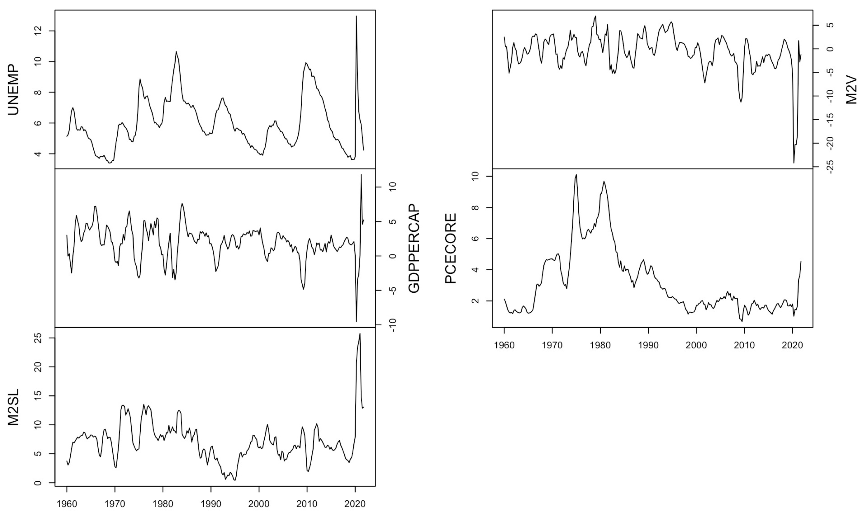
Figure 2 shows the time series of GDP per capita, the unemployment rate, M2, the velocity of money, and core inflation during the sample period from 1960:Q1 to 2021:Q4. Overall, the indirect relationship between GDP and the unemployment rate, as well as money supply and the velocity of money, is evident. However, the core inflation does not follow any clear pattern. In the early 1990s, the inflation rate was at around 4%, followed by a decline to 2% until late 1999. With the beginning of the year 2000, the inflation rate in the U.S. rose again, and it reached a peak in late 2007, which is officially known as the year when the U.S. economy slowed down and entered the Great Recession. With the beginning of the crisis, inflation followed the decline and stayed below 2% until the end of the sample period. Exceptions are the years 2011 and 2012, where the inflation rate in the U.S. was at around 3%. The recent shocks in these monetary indicators had never been experienced in the last six decades in the U.S. We provide a sensitivity analysis for the period of the Great Recession (2008:Q1 to 2009:Q2), but we should emphasize that the magnitude of the shocks are not comparable to that period.
4. Discussion
At the inception of our paper in mid-2021, the interest rate remained low and the Federal Reserve was cautious about raising the rates based on the “transitory” view of the rising inflation, as we discussed in
Section 1. The unprecedented increase in the money supply as shown in
Figure 1 and the uniqueness of the COVID-19 recession, especially with the domestic lockdowns in March and April 2020, as argued in
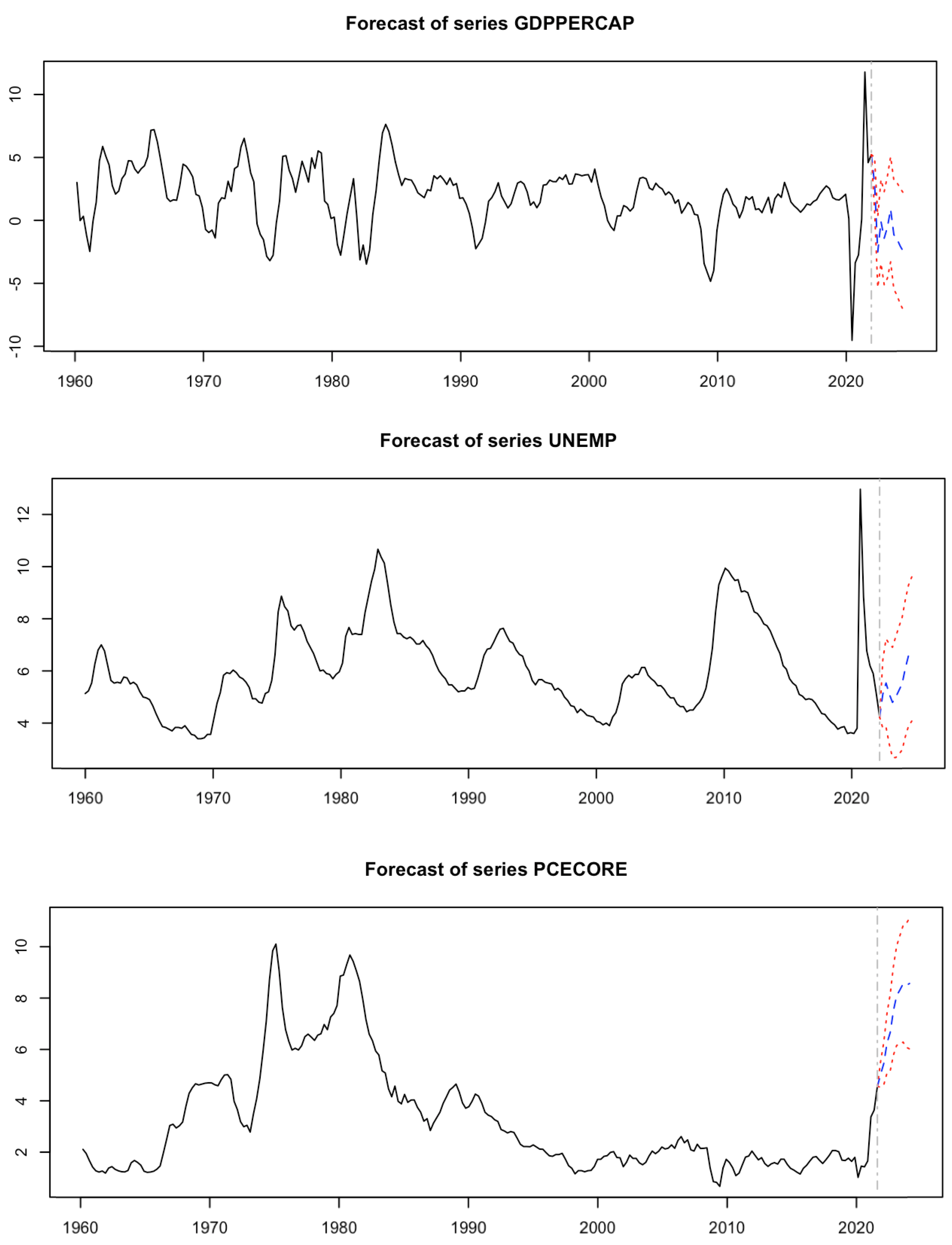
Section 2.1, may have led to a more persistent upward shift in inflation. Our forecasts indicate that the core inflation rate will hover around a high 4% and the rate will continue to climb up in the near future. Hence, we have shown that a change in policy is necessary to correct for the upward pressure on the long-run inflation. In line with our prediction and given the persistent inflation, the Federal Reserve increased the interest rate on March 2022 by 0.25 percentage point
6.
We compared our predictions in 2022 with other predictions and examined how our predictions fared against other forecasts. In a press conference on 16 March 2022
7, Federal Reserve Chairman Jerome Powell stated that the median inflation projection of FOMC participants is 4.3 percent in 2022, 2.7 percent in 2023, and 2.3 percent in 2024. Chairman Powell added that the recent trajectory is much higher than their own projection in December 2021 and noted that the FOMC participants continue to see risks as weighted to the upside. These estimates are similar to our predictions. Furthermore, a result from the monthly Bloomberg survey of 70 economists on April 2022 shows that the average core inflation for 2022 will be approximately 4.7%.
8 Their estimate falls within our confidence interval.
The lockdowns in March and April 2020 and the consequent expansionary fiscal and monetary policies led to an unprecedented increase in the level of money supply. These government policies are not unusual as the Federal Reserve used conventional monetary tools such as lowering the interest rates and increasing asset purchases during the Global Financial Crisis (
Mishkin 2009). However, the lesson from COVID-19 seems to indicate that forecasting inflation in times of a pandemic is different from in times of a financial crisis. The main difference was the lockdowns, which directly affected the unemployment rate, and our proposed model reflected this macroeconomic behavior. Hence, a major policy implication of our study is that the traditional ordering of the VAR model may not be sufficient when modeling the money supply and inflation in the current or future pandemics.
5. Conclusions
January 2022 marks the highest U.S. inflation rate in 40 years. The Federal Reserve began tightening the monetary policy in March 2022 to combat the high inflation. We showed that the traditional model of inflation forecasts may not capture all of the macroeconomic behaviors during a pandemic. The direct impact on the unemployment rate because of the lockdowns in March and April 2020 is the main difference from previous recessions. Incorporating this main difference into the model could have allowed us to realize that the COVID-19’s era inflation is not transitory.
Our proposed model predicts that the annualized quarterly core inflation rate could rise to 5.03% for the first quarter of 2022 and to 5.45% for the second quarter. In a longer time horizon, we forecast that the inflation rate could reach as high as 8.57% unless corrected with appropriate monetary policies. We also showed that the high inflation after COVID-19 is not transitory, but it is persistent. That is, the recent economic recovery and the excessive supply of M2 from fiscal and monetary policies have increased the core inflation rate beyond a transitory phase.
We contribute to the literature by proposing a changed VAR model specification to forecast inflation after COVID-19. The main modification is incorporating the exogenous shocks, namely domestic lockdown policies, to unemployment during the pandemic. Our proposed VAR model reflects the real macroeconomic behaviors during the pandemic, carefully contemplates the contemporaneous effects of these indicators, and performs well in forecasting future price levels. One of the main implications of our analysis is that the macroeconomic indicators during the recent pandemic-era recession may have different parameters than those from any other recessions. Failing to re-scale these differences may have contributed to the insufficient policy responses to the inflation shocks by the Federal Reserve.
We conclude with three caveats of our research. First, we designed our VAR strategy for forecasting inflation during a pandemic time only. Second, we did not incorporate inflation expectations. Third, our approach does not incorporate up-to-date methods, such as using high-frequency movement in interest rate futures around FOMC announcement dates or using external instrumental variables to identify monetary policy shocks. We believe these are important topics for future research.
