Article

Do Government Expenditures in G7 Countries Target Socioeconomics or Physical Output?

by
Arqam Abdul Razzaq Al-Rabbaie
1,
Usama Robin Al-qalawi
1,* and
Ahmad Alwaked
2
1
Department of Economics, Faculty of Economic and Administrative Sciences, The Hashemite University, P.O. Box 330127, Zarqa 13133, Jordan
2
Department of Business & Financial Economics, Yarmouk University, P.O. Box 566, Irbid 21163, Jordan
*
Author to whom correspondence should be addressed.
Economies 2022, 10(10), 262; https://doi.org/10.3390/economies10100262
Submission received: 30 July 2022 / Revised: 18 September 2022 / Accepted: 8 October 2022 / Published: 21 October 2022

Abstract

:
The issue of valuable government policy interventions has not been fully addressed. Therefore, this paper analyzes the impact of government capital expenditure on production efficiency in the G7 countries. Two models are estimated with different dependent variables: the Human Development Index (HDI) as a dependent variable to capture the socio-economic impact and the gross domestic product (GDP) as a dependent variable to capture the physical impact. The paper uses a set of panel data for the G7 countries spanning the years 2000–2018, which were obtained from the World Development Indicators (WDI) database. The paper applies stochastic production frontier analysis (SFA) to estimate each country’s yearly efficiency and to estimate the impact of government expenditure on the overall technical inefficiency for both models. The results demonstrate that increasing government expenditure boosts the inefficiency in the G7 countries in the HDI model, but it depresses inefficiency in the GDP model. This may suggest that government capital expenditure in the G7 countries was directed toward increasing physical output—not toward socio-economic outputs such as health and educational output—during the study period. Furthermore, the results show that the estimated average technical efficiency over the study period was 93.4% for the HDI model and 81.2% for the GDP model. Finally, the results show that the G7 countries’ objectives were not similar in this area, with some countries using socioeconomic-oriented policies and others using physical-capital-oriented policies.
JEL Classification:
C54; E61; H51; H52

1. Introduction

Many economists believe that government is an important part of the development process and has the power to steer an economy toward a desired equilibrium. They contend that there are numerous flaws in both product and factor markets. Governments play a crucial role in facilitating the operation of markets through interventions by investing in physical and social infrastructure, healthcare facilities, and educational institutions, as well as by fostering an environment favorable for private enterprise.
Government spending goals vary between countries. According to Kim (2018), governments prefer to invest in physical capital than human capital because they want to achieve economic growth, which may weaken the country’s competitiveness in a rapidly changing world. He added that politicians might not be motivated to support measures whose benefits will not manifest for many years.
Lucas (1988) and Zagler and Dürnecker (2003) suggest that government spending and sub-spending on different sectors—such as education, health, infrastructure, research, and development—should be considered an engine of growth. Therefore, the efficient use of public spending is questionable by taxpayers to meet the demand for public goods and services.
This variation in economic spending goals raises a legitimate question about the correct measurements of economic growth. The gross domestic product (GDP), which is a measurement of marketable production of the economy, is frequently used as shorthand for the well-being of the nation’s economy, despite the fact that this was never its original purpose. Correctly measuring economic well-being is important because it has an impact on societal and governmental decisions. GDP cannot monitor well-being if externalities exist, such as environmental harm brought on by production and consumption activities (Aitken 2019). Kim (2018) stresses that financial growth is insufficient and that some countries will need to increase the efficiency of their social services while preserving their level of quality.
In addition, Lauri Peterson (2014) argues that the well-being discussion should go further than GDP, finding that the most appropriate metric for well-being is HDI because it captures the economic, health, and education disparities.
Kelley (1991) argues that it is reasonable to include HDI as a proxy to output since government expenditure affects not only the physical output through the multiplier effect but also the quality and quantity of health and education.
Despotis (2005) argues that development measurements traditionally concentrate on economic indicators as proxies for development, namely, income per capita and GDP per capita. These measures are criticized on the basis that they do not capture the dimensions of human development. The Human Development Index (HDI), which was introduced by the United Nations Development Program in 1990, is used as a proxy to measure development.
This paper considers these differences and tries to differentiate between the effects of government spending on production efficiency using different measures of total production. This process is not only an original contribution but also a way to capture some unobservable information related to the effects of government spending on production with and without the socioeconomic dimension.
Measuring productive efficiency is a crucial issue for economic policymakers. The seminal paper discussing the measurement of productive efficiency was introduced by Farrel (1957), who argued that “The measures developed are intended to be quite general, applicable to any productive organization from a workshop to a whole economy” (Farrel 1957, p. 254).
With respect to the techniques that are used in this paper, we noted that many previous studies consider the productive efficiency of public spending by applying either data envelopment analysis (DEA) and/or stochastic frontier approaches, with emphasis mostly concentrated on education and health, as well as different types of government spending, such as social, transfers and subsidies, and infrastructure. We preferred to use the stochastic frontier approach, since it has the advantage of simultaneously measuring the effects of several control variables on production efficiency (Burgess 2006). In addition, SFA has the ability to ability to control for randomness in the data and a wide range of variables (Greene 2004).
The rest of this paper is structured as follows: Section 2 presents the literature review. Section 3 describes the methodology. Section 4 describes the data sources and definitions. Section 5 presents the estimates. Finally, Section 6 concludes our research.

2. Literature Review

The efficient usage of resources in the production process has attracted increasing discussion in the literature during the last two decades. (Afonso et al. 2020; Gupta and Verhoeven 2001) Governments usually use fiscal policy to solve short-term economic problems and achieve economic development. In addition, valuable intervention by governments is significantly important to reach their developmental goals. The government’s size is crucially important to a country’s performance.
Most previous papers deal with public sector performance and efficiency, such as Gupta and Verhoeven (2001), Afonso and Aubyn (2005), Afonso et al. (2010a, 2010b, 2013), and Afonso and Kazemi (2017). These research papers estimate fiscal policy efficiency scores. The results of these studies show that different types of government expenditures are positively and statistically related to performance.
Afonso and Kazemi (2017) studied the efficiency of the public sector in 20 OECD countries over the period 2009–2013 using DEA. They considered different types of government expenditure and public spending as a whole as inputs, while they considered public sector performance scores as outputs. The results of public sector efficiency in OECD countries showed that Switzerland was the most efficient country, while all other countries could reduce government spending by 26.8% and stay at the same level of performance.
Verhoeven et al. (2007) investigated the efficiency of the health and education sectors in the G7 countries over the period 1995–2003 using the DEA approach. The results showed that the developed G7 countries were not the most efficient in the OECD group.
Prasetyo and Ubaidillah (2013) explored the efficiency of three strands of government spending per capita—in health, education, and transfer and subsidies—in 88 countries as inputs, while the Human Development Index was considered as the output. They used the DEA approach over the period 2006–2010. The results indicated that most of the countries were on the production frontier.
De Borger and Kerstens (1996) investigated the efficiency of municipalities’ spending in Belgium using parametric and non-parametric approaches. The results showed a large difference in efficiency scores, suggesting that there is a problem in choosing the best technique; hence, they used a wide variety of techniques.
Aman and Murova (2015) investigated the public productivity for all 50 US states using DEA over the period 1992–2012. The results showed that efficiency decreased over the period of the study, with minor exceptions for some states.
Afonso et al. (2010b) investigated the efficiency of public social spending as the input to the Gini coefficient as an income distribution indicator for a group of OECD counties using DEA. For Anglo-Saxon countries, the results indicated both input and output efficiency.
Chan et al. (2017) examined the effects of government spending efficiency on economic growth for 115 countries. They used the DEA approach to extract government efficiency scores for each country. Furthermore, they included the government efficiency score variable, among other variables, to estimate the effects of government spending efficiency on economic growth. The results suggested that economic growth relies on the ability of the government to use its resources efficiently.
Murova and Khan (2017) investigated the efficiency of public investment in five service sectors over the period 1992–2012 in the USA. They employed the Cobb–Douglas stochastic frontier analysis (SFA). The results showed the positive impact of government investment on the Gross Domestic Product. Moreover, the mean technical efficiency of public sector spending was 0.878, suggesting a high level of efficiency across all years and states.
Economic theory states that there is a relationship between output and government expenditure. Keynesian economics predicted that government expenditure causes output growth, whereas Wagner predicted that economic growth would lead to increased government expenditure. Moreover, development economists argue that governments use deep intervention to move the economy to a preferred equilibrium. Accordingly, we found no empirical paper that directly addresses the relationship between production efficiency and government economic policies in the way in which we analyze it in this paper.

3. Methodology

To explain the probability that production takes place beneath the production frontier, Aigner et al. (1977) and Meeusen and Broeck (1977) established the stochastic production frontier model. A review of stochastic frontier models can be found in the work of Kumbhakar and Lovell (2000). This study estimates the stochastic production frontier for cross-sectional time-series data for G7 countries across a 19-year timespan. The countries’ technical inefficiency is estimated by the distance between the actual frontier and the optimal one.
If Yit denotes the output of the i-th country at time t, then the output can be expressed as follows:
  Y i t = f ( x j i t ;   β ) exp ( ε i t )
where i represents the countries, t represents the time period, j represents the input, and β is a vector of the parameters to be estimated. The error term   ε i t has two components: v and u, where vit is the random error and uit represents the inefficiency. The random error, vit, is a normal variable that is independently and identically distributed with a mean of zero and a variance equal to   σ v 2 . The error term is represented as follows:
ε i t = v i t u i t
To estimate technical efficiency (TEit), we assume that ui is a non-negative, zero-truncated, normally distributed variable with mean δzit and variance   σ u 2 , where zi represents variables that contribute to inefficiency and δ is an unknown coefficient to be estimated. Thus, the technical inefficiency ui can be represented as follows:
u i t = δ z i t + w i t
where wit is a truncated normal random variable with zero mean and σ u 2   variance (Battese and Coelli 1993, 1995). In addition, since we used a logarithmic production function, technical efficiency can be defined as follows:
T E i t = E [ e x p ( u i t ) \ ε i t ]
T E i t = { θ ( r i σ ) θ ( r i ) } exp { μ i t + 1 2 σ 2 }
where θ ( · )   represents the standard normal cumulative distribution, and
r i = μ i t σ ,   μ i t = σ u 2 ε i t + δ z i t σ v 2 σ u 2 + σ v 2 ,             σ 2 = σ u 2 σ v 2 σ u 2 + σ v 2
The most common production function used in this kind of literature is the translog production function. However, due to the degree-of-freedom problem, we used the Cobb–Douglas production function to estimate the production function coefficients. This function is commonly used in the literature, making estimates comparable with those of previous studies. We chose capital (k) and labor (L) as inputs, and the coefficients of these variables were expected to be positive. Thus, the specification of the production function is given as follows:
L n ( Y i t ) = B 0 + B 1   L n   L + B 2   L n   K + ( v u )
The effects of technical inefficiency are defined as follows:
u i t = δ 0 + δ 1 ln G i t
where Git is the government spending variable, and the coefficient of this variable could be positive or negative. If it takes a significant positive value, this indicates that government spending increases the inefficiency of the production function, but if it takes a significant negative value, it indicates that government expenditure decreases the inefficiency. Finally, if the coefficient of the government expenditure is not significant, this means that government expenditure does not have any effect on efficiency of the production function.
The models were estimated twice with different measures of output ( Y i t ). In the first estimation, we used HDI as the output, while in the second we used GDP as the output. However, the inputs for the estimated models and the technical inefficiency effects represented by labor, capital, and government spending were the same for both models.

4. Data

GDP, labor, capital, and government expenditure data for G7 countries from 2000 to 2018 were obtained from the World Development Indicators for World Bank national accounts. HDI data were obtained from the Human Development Report of the United Nations Development Program. Data were measured in 2015 constant prices. Fixed capital formation was used for k. The number of employed people aged 15 or older who supplied labor to produce goods and services during a specific period was used to measure the labor input. We also collected data for government capital expenditure for possible correlation with inefficiency.

5. Results

The maximum likelihood estimation (MLE) approach was used in the estimation of Model (3) using Frontier 4.1 software (Coelli 1996). The coefficients shown in Table 1 for the production inputs were significant. The estimated parameter γ was almost equal to one in both models, and this represents the variance of the inefficiency of the error, σ u 2 , divided by the overall variance that equals σ u 2 + σ v 2 . This also implies that most of the variation in error results from the inefficiency, and proves that the use of the stochastic frontier model is suitable for both models.
For the first model, Table 2 shows the labor and capital elasticity of socioeconomic production, such that as labor increases by 1%, socioeconomic production decreases by 2.8%. This may be related to saturation in labor. However, as capital increases by 1%, socioeconomic production increases by 7.7%. The sum of both forms of elasticity shows that the production function for socioeconomic production is in the phase of decreasing return to scale. This means that increasing the input by 1% will increase socioeconomic production by less than 1%, and this suggests that a loss of efficiency is expected in the socioeconomic production process, even when the production has been expanded. Moreover, the coefficient of government capital investment is positive and significant, and this implies that as government capital expenditure increases, the inefficiency of HDI increases for G7 countries. This may suggest that the increase in government capital investment was not directed toward developing education or health outputs.
Inversely, the second model shown in Table 3 shows that as labor increases by 1%, physical production increases by 70%, and as capital increases by 1%, physical production increases by 31%. Both forms of elasticity are larger than in socioeconomic production, suggesting that resources are more socioeconomically productive, and this may be related to the government spending that facilitates and supports physical production. The sum of both forms of elasticity shows that the production function for physical production is in the phase of increasing return to scale. This means that increasing the input by 1% will increase socioeconomic production by more than 1%, and this suggests that efficiency increases when countries progress from small-scale to large-scale production. Moreover, the coefficient of capital government investment is negative and significant, and this indicates that as government capital expenditure increases, the inefficiency of GDP output decreases for G7 countries. One possible explanation for this is that the increase in government capital investment can help to increase efficiency directed toward developing physical output and to achieve economic growth, as noted by Kim (2018).
Table 4 and Table 5 show the estimates of technical efficiency for each country for every year in the sample. Readers can easily observe the fluctuation in technical efficiency for each country over time. Table 4 shows that when we used the HDI as the output we found that the most efficient country during the period of study was Canada, followed by the UK, with average efficiency of 0.9853 and 0.9820, respectively. The least efficient country was the US, followed by Japan, with average efficiency of 0.8842 and 0.9039, respectively, during the study period.
Figure 1 shows the average efficiency for each G7 country during the timespan. All average efficiency scores reflect fluctuation, but we can clearly observe that Canada and the UK were the most efficient countries during the study period. They exchanged positions in 2008 and 2015. The third position was taken by Germany. The efficiency of Germany continued to increase until 2006, and then it decreased thereafter. France started from almost the same position as Germany, but it had a decreasing trend that placed it in the fourth position until 2006, when it moved to the fifth position below Italy, and in 2018 took the sixth position after Japan. The HDI efficiency of the USA was in last place since 2004, and this may be related to the Second Gulf War.
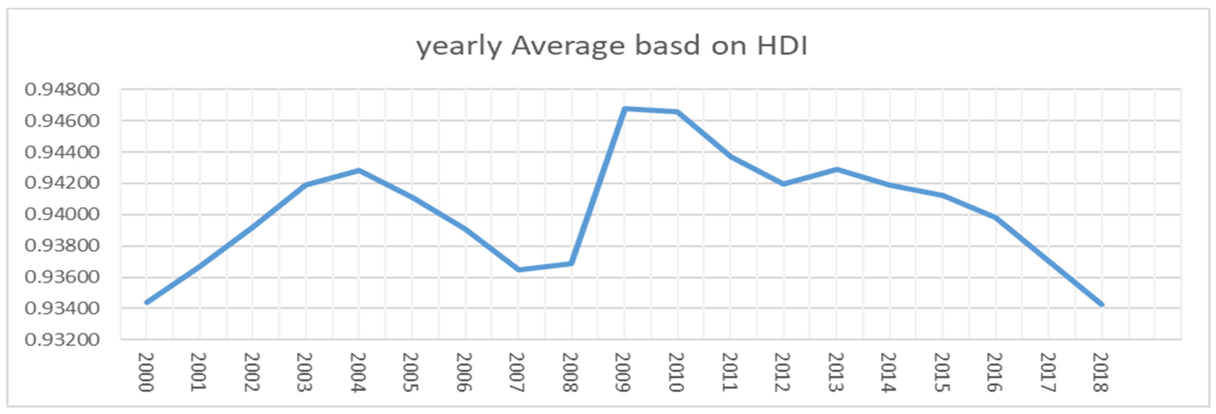
The yearly average efficiency for all countries together is shown in Figure 2. The average yearly efficiency was equal to 93.44% in 2000. Then, it continued to increase until it reached 94.28% in 2004, after which it continued to decrease until it reached 93.9% in 2007. The average yearly efficiency reached its record high in 2009, with average efficiency of 94.68%, but it then decreased until it reached its record low at the end of the study period, with average efficiency equal to 93.42%. It should be noted that first of the two declines in yearly average efficiency may be related to the Second Gulf War. The second decline may be related to the financial crisis of 2007–2008. Accordingly, we may conclude that governments’ capital expenditure during crises has been directed toward expenditure other than improving education and health outputs.
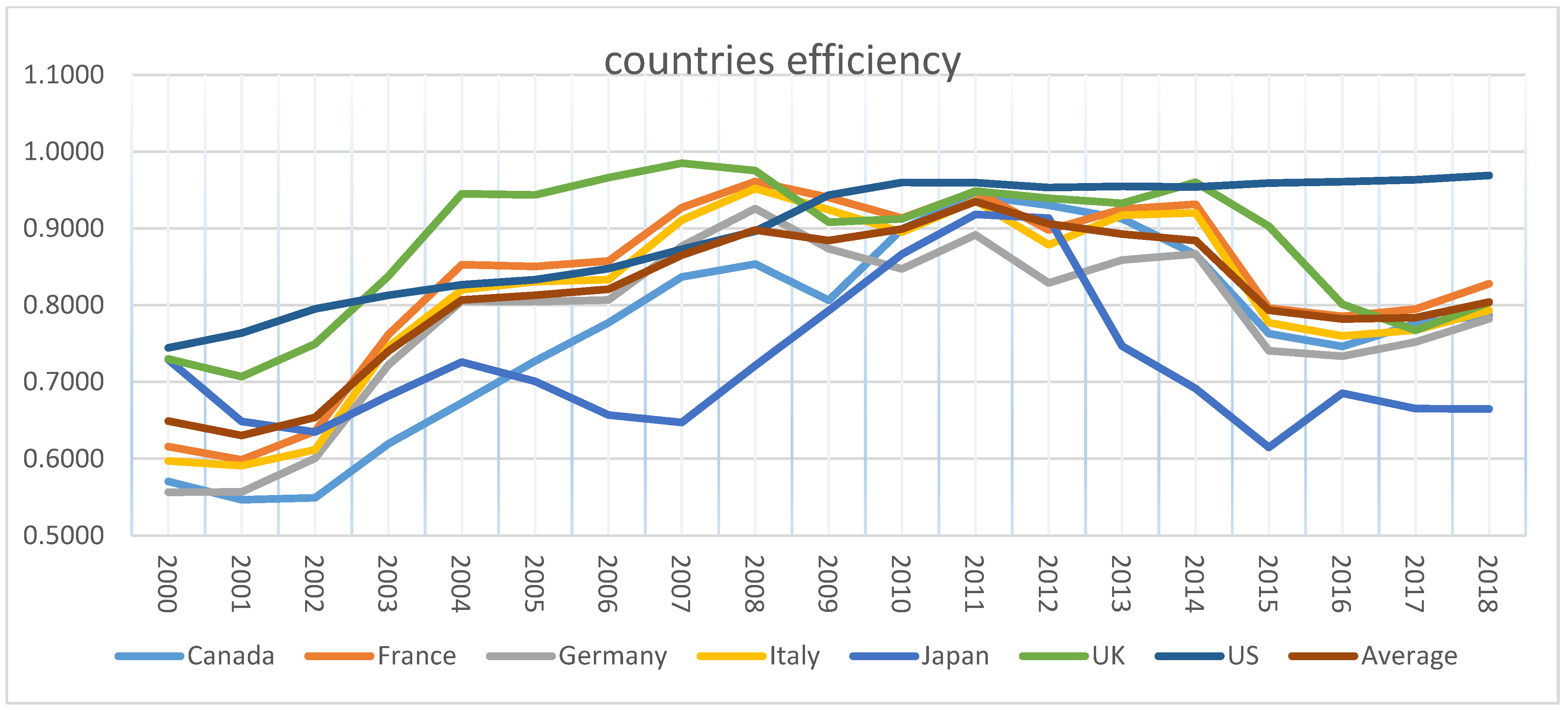
Table 5 presents each country’s yearly efficiency using GDP as the output. The most efficient country was the US, with average efficiency of 89.3%. This result, together with the results shown in Table 4, suggests that the US gives more priority to government capital expenditure that serves the cause of income than to expenditure that serves the health and education services compared to other G7 countries. Similarly, France’s average efficiency ranks third in Table 5 and fifth in Table 4. The average sample efficiency of the UK is ranked second, with efficiency of 87.9%, and this is the same rank as the UK’s efficiency in Table 4. In addition, this may suggest that the UK is relatively efficient in terms of both the HDI output and the GDP output. Similarly, Italy was ranked fourth in both measures. Canada is ranked last in Table 5 but first in Table 4. This may lead us to conclude that Canada’s government capital expenditure is more efficient in producing health and educational outputs than in producing income relative to other G7 countries.
Figure 3 present countries’ yearly efficiency during the period of the study for GDP output. It is clear that this model had more fluctuation than the HDI model for all countries except for the US, which showed an increasing trend for most of the study period. This could be related to the strong commitment of the US government to increasing GDP.
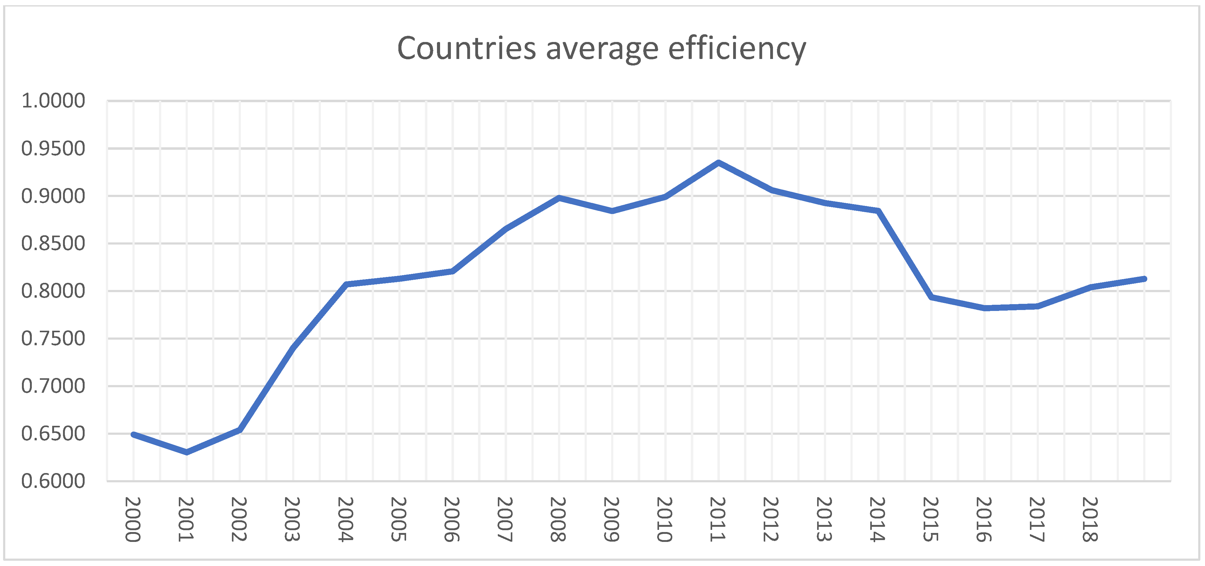
Figure 4 shows all countries’ average efficiency during the study period. The average efficiency was equal to 65% in the year 2000, and dropped slightly below that in the year 2001. Then, it continued to increase, reaching 90% in the year 2008 and 93.5% in 2011, after which it dropped sharply to reach 78.4% in 2017.

6. Conclusions

This study estimated technical efficiency for G7 countries from 2000 to 2018 using two models with different outputs; the first output was the HDI and the second output was GDP. The two models used labor and capital as inputs and government capital expenditure as a correlate to efficiency. The results showed that almost all of the variation in error resulted from inefficiency. This proves that the use of the stochastic frontier model is suitable for this study. In addition, the elasticity of labor and capital indicated that labor and capital are less productive in socioeconomic production than in physical production, and the economies of scale suggest that physical production is more efficient than socioeconomic production. The average technical efficiency during this period was 93.4% for the HDI model and 81.2% for the GDP model. Moreover, technical efficiency fluctuated for the majority of countries. The efficiency rankings were generally different over time for the two models. The first model shows that government capital expenditure increases the inefficiency of HDI, while the second model shows that government capital expenditure decreases the inefficiency of GDP. All of these results suggest that government capital expenditure for the G7 countries was generally directed toward increasing income rather than health and educational outputs during the period of the study. This result is similar to the findings of Verhoeven et al. (2007). The G7 countries need to reform their educational and health expenditure policies in order to enhance the efficiency of these expenditures. Finally, the results show that the G7 countries’ objectives were not similar in this area; hence, some G7 countries use socioeconomic-oriented policies, while others use physical-capital-oriented policies.

This Study

The authors of this study acknowledge it has potential limitations with regard to the small sample and the few independent variables included in terms of both the production function and the inefficiency explanation function; these limitations may affect the results, but since the idea of this paper is new to the best of our knowledge, we preferred that it be kept as simple as possible. This may open the door for further research.

Author Contributions

Conceptualization, A.A.R.A.-R. and U.R.A.-q.; methodology, U.R.A.-q.; software, U.R.A.-q. and A.A.; validation, U.R.A.-q., A.A. and A.A.R.A.-R.; formal analysis, A.A.; investigation, A.A.R.A.-R.; resources, A.A.R.A.-R.; data curation, A.A.R.A.-R.; writing—original draft preparation, A.A.R.A.-R.; writing—review and editing, U.R.A.-q. and A.A.; visualization, U.R.A.-q.; supervision, A.A.R.A.-R.; project administration, A.A.R.A.-R.; funding acquisition, U.R.A.-q. All authors have read and agreed to the published version of the manuscript.

Funding

This research received no external funding.

Institutional Review Board Statement

Not applicable.

Informed Consent Statement

Not applicable.

Data Availability Statement

Data is available in the World Development Indicators for World Bank national accounts. HDI data were obtained from the Human Development Report of the United Nations Development Program.

Acknowledgments

We would like to thank the referees for their suggestions for improving this article, as well as Tim Coelli for making the Frontier 4.1 software available.

Conflicts of Interest

The authors declare no conflict of interest.

References

  1. Afonso, António, Alma Romero-Barrutieta, and Emma Monsalve. 2013. Public Sector Efficiency: Evidence for Latin America Public. Available online: https://ssrn.com/abstract=2365007 (accessed on 10 July 2021).
  2. Afonso, António, and Miguel St Aubyn. 2005. Nonparametric Approaches to Educational and health expenditures Efficiency in OECD countries. Journal of Applied Economics 8: 227–46. [Google Scholar] [CrossRef] [Green Version]
  3. Afonso, António, João Tovar Jalles, and Ana Venâncio. 2020. Government Spending Efficiency, Measurement and Applications: A Cross-Country Efficiency Dataset. REM Working Paper 0147-2020. Available online: https://ssrn.com/abstract=3734216 (accessed on 20 June 2021).
  4. Afonso, Antonio, Ludger Schuknecht, and Vito Tanzi. 2010a. Public Sector Efficiency: Evidence for New EU Member States and Emerging Markets. Applied Economics 42: 2147–64. [Google Scholar] [CrossRef] [Green Version]
  5. Afonso, Antonio, Ludger Schuknecht, and Vito Tanzi. 2010b. Income Distribution Determinants and Public Spending efficiency. The Journal of Economic Inequality 8: 367–89. [Google Scholar] [CrossRef] [Green Version]
  6. Afonso, António, and Mina Kazemi. 2017. Assessing public spending efficiency in 20 OECD countries. In Inequality and Finance in Macrodynamics. Cham: Springer, pp. 7–42. [Google Scholar]
  7. Aigner, Dennis, C. A. Knox Lovell, and Peter Schmidt. 1977. Formulation and estimation of stochastic frontier production function models. Journal of Econometrics 6: 21–37. [Google Scholar] [CrossRef]
  8. Aitken, Andrew. 2019. Measuring Welfare Beyond GDP. National Institute Economic Review 249: R3–R16. [Google Scholar] [CrossRef]
  9. Aman, Khan, and Olga I. Murova. 2015. Productive Efficiency of Public Expenditures: A Cross-state Study. State and Local Government Review 47: 170–80. [Google Scholar]
  10. Battese, George Edward, and Tim J. Coelli. 1993. A Stochastic Frontier Production Function Incorporating a Model for Technical Inefficiency Effects. Working Papers in Econometrics and Applied Statistics No. 69. Armidale: Department of Economics, University of New England. [Google Scholar]
  11. Battese, George Edward, and Tim J. Coelli. 1995. A model for technical inefficiency effects in a stochastic frontier production function for panel data. Empirical Economics 20: 325–32. [Google Scholar] [CrossRef] [Green Version]
  12. Burgess, James F. 2006. Productivity analysis in health care. In The Elgar Companion to Health Economics, 2nd ed. Cheltenham: Edward Elgar Publishing. [Google Scholar]
  13. Chan, Sok-Gee, Zulkufly Ramly, and Mohd Zaini Abd Karim. 2017. Government spending efficiency on economic growth: Roles of value-added tax. Global Economic Review 46: 162–88. [Google Scholar] [CrossRef]
  14. Coelli, Tim J. 1996. A Guide to FRONTIER Version 4.1: A Computer Program for Stochastic Frontier Production and Cost Function Estimation. CEPA Working Papers. Armidale: CEPA, vol. 7. [Google Scholar]
  15. De Borger, Bruno, and Kristiaan Kerstens. 1996. Cost efficiency of Belgian local governments: A comparative analysis of FDH, DEA, and econometric approaches. Regional Science and Urban Economics 26: 145–70. [Google Scholar] [CrossRef]
  16. Despotis, D. K. 2005. Measuring human development via data envelopment analysis: The case of Asia and the Pacific. The International Journal of Management Science 33: 385–90. [Google Scholar] [CrossRef]
  17. Farrel, Michael James. 1957. The Measurement of productive efficiency. Journal of the Royal Statistical Society: Series A (General) Part III 120: 253–90. [Google Scholar] [CrossRef]
  18. Greene, William. 2004. Distinguishing between heterogeneity and inefficiency: Stochastic frontier analysis of World Health Organization’s panel data on national health care systems. Health Economics 13: 959–80. [Google Scholar] [CrossRef] [PubMed]
  19. Gupta, Sanjeev, and Marijn Verhoeven. 2001. The efficiency of government expenditure—Experiences from Africa. Journal of Policy Modelling 23: 433–67. [Google Scholar] [CrossRef] [Green Version]
  20. Kelley, Allen C. 1991. The Human Development Index: “Handle with Care”. Population and Development Review 17: 315–24. [Google Scholar] [CrossRef]
  21. Kim, Jim Yong. 2018. The Human Capital Gap: Getting Governments to Invest in People. Foreign Affairs 97: 92–101. Available online: http://www.jstor.org/stable/44822216 (accessed on 6 April 2021).
  22. Kumbhakar, Subal C., and C. A. Knox Lovell. 2000. Stochastic Frontier Analysis. Cambridge: Cambridge University Press. [Google Scholar] [CrossRef]
  23. Lucas, Robert E., Jr. 1988. On the Mechanics of Economic. Development. Journal of Monetary Economics 22: 3–42. [Google Scholar] [CrossRef]
  24. Meeusen, Wim, and Julien van Den Broeck. 1977. Efficiency estimation from Cobb-Douglas production functions with composed error. International Economic Review 18: 435–44. [Google Scholar] [CrossRef]
  25. Murova, Olga, and Aman Khan. 2017. Public investments, productivity and economic growth: A cross-state study of selected public expenditures in the United States. International Journal of Productivity and Performance Management 66: 251–65. [Google Scholar] [CrossRef]
  26. Peterson, Lauri. 2014. The measurement of Non-economic Inequality in Well Being Indices. Social Indicators Research 119: 581–98. [Google Scholar] [CrossRef]
  27. Prasetyo, Ahmad Danu, and Zuhdi Ubaidillah. 2013. The Government Expenditure Efficiency towards the Human Development. Procedia Economics and Finance 5: 615–22. [Google Scholar] [CrossRef] [Green Version]
  28. Verhoeven, Marijn, Victoria Gunnarsson, and Stephanie Carcillo. 2007. Education and Health in G7 Countries: Achieving Better Outcomes with Less Spending. IMF Working Paper WP/07/263. Available online: https://ssrn.com/abstract=1033217 (accessed on 19 May 2021).
  29. Zagler, Martin, and Georg Dürnecker. 2003. Fiscal Policy and Economic Growth. Journal of Economic Survey 17: 397–418. [Google Scholar] [CrossRef]
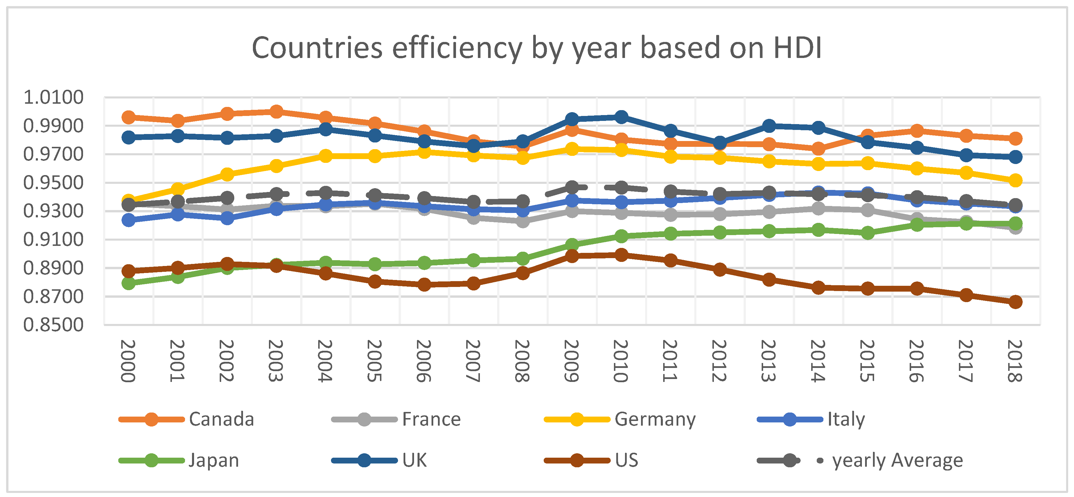
Figure 1. HDI efficiency by country. Source: Authors’ work based on estimated efficiencies.
Economies 10 00262 g001
Figure 2. All-country average HDI efficiency. Source: Authors’ work based on estimated efficiencies.
Economies 10 00262 g002
Figure 3. Each country’s yearly efficiency based on GDP output. Source: Authors’ work based on estimated efficiencies.
Economies 10 00262 g003
Figure 4. All countries’ average efficiency based on GDP output. Source: Authors’ work based on estimated efficiencies.
Economies 10 00262 g004
Table 1. Descriptive statistics for G7 countries.
CountryStatisticsHDIGDP
(Billion USD)
Labor
(Million)
Capital
(Million USD)
Government Expenditure (Million USD)
CanadaMean0.897581390.0017.23241,969.80548.73
Maximum0.922001840.0019.16358,648.10730.04
Minimum0.86800736.0015.08123,902.90299.20
S.D.0.0166387.001.1977,968.65155.10
FranceMean0.869112370.0026.63395,905.401279.54
Maximum0.891002920.0027.69620,976.801605.02
Minimum0.842001360.0024.56223,914.90684.00
S.D.0.01658511.000.87117,057.60308.37
GermanyMean0.913003180.0038.81542,697.801437.39
Maximum0.939003950.0042.09896,915.401736.48
Minimum0.869001940.0036.21365,718.70913.87
S.D.0.02145653.001.82164,161.80265.79
ItalyMean0.863841900.0022.36309,683.30914.00
Maximum0.883002400.0023.27420,231.001123.48
Minimum0.830001140.0020.76206,261.70519.06
S.D.0.01547370.000.6557,068.18195.94
JapanMean0.885214940.0064.04952,356.101818.38
Maximum0.915006200.0066.711,152,520.002465.21
Minimum0.855004120.0062.78822,928.001416.47
S.D.0.01899570.000.91105,802.90311.66
UKMean0.897262530.0029.92305,300.601065.87
Maximum0.920003100.0032.96506,140.201303.36
Minimum0.867001640.0027.67181,344.10612.16
S.D.0.01723446.001.5697,517.66223.04
USMean0.9046814,900.00147.002,361,391.005354.80
Maximum0.9200020,500.00159.003,814,110.007305.98
Minimum0.8810010,300.00140.001,496,212.002951.49
S.D.0.013173080.005.83697,329.701292.58
AllMean0.89014460.0049.36729,900.501774.10
Maximum0.939020,500.00159.003,814,110.007305.98
Minimum0.8300736.0015.08123,902.90299.20
S.D.0.02394590.0042.36756,928.901603.46
Source: Authors’ calculation.
Table 2. The SFA MLE estimates.
Dependent VariableLn (HDI)
Independent VariableCoefficientStandard Errort-Ratio
Intercept (β0)4.0302 ***0.048183.7685
Ln(L)−0.0282 ***0.0079−3.5471
Ln(K)0.0770 ***0.00878.8801
Intercept (δ0)−0.3994 ***0.0079−50.8670
Ln(G)0.0402 ***0.0003125.5703
Sigma-squared0.0005 ***0.00019.5439
Gamma0.9999 ***0.10639.4044
Note: ***, **, and * denote significance at the 1%, 5%, and 10% levels, respectively. Source: Authors’ calculation.
Table 3. The SFA MLE estimates.
Dependent VariableLn (GDP)
Independent VariableCoefficientStandard Errort-Ratio
Intercept (β0)12.5854 ***0.478526.3008
Ln(L)0.7014 ***0.059911.7186
Ln(K)0.3181 ***0.04756.6999
Intercept (δ0)1.2938 **0.49812.5975
Ln(G)−0.1054 **0.0469−2.2465
Sigma-squared0.0515 ***0.01822.8313
Gamma0.9624 ***0.024539.2460
Note: ***, **, and * denote significance at the 1%, 5%, and 10% levels, respectively. Source: Authors’ calculation.
Table 4. Efficiency of fiscal policy based on the HDI.
YearCanadaFranceGermanyItalyJapanUKUSYearly AverageRank
20000.99590.93520.93720.92370.87930.98180.88780.934418
20010.99350.93350.94530.92770.88380.98280.89010.936716
20020.99840.93110.95580.92500.89000.98150.89280.939212
20030.99990.93370.96170.93150.89220.98290.89150.94198
20040.99560.93340.96870.93480.89370.98750.88620.94285
20050.99150.93530.96870.93590.89270.98320.88050.941110
20060.98600.93150.97160.93350.89360.97900.87830.939113
20070.97900.92530.96920.93130.89540.97580.87910.936417
20080.97550.92290.96740.93060.89650.97900.88640.936915
20090.98710.93000.97370.93750.90620.99450.89840.94681
20100.98030.92870.97300.93630.91230.99610.89920.94662
20110.97730.92740.96830.93730.91410.98640.89530.94373
20120.97730.92780.96750.93940.91500.97810.88890.94206
20130.97700.92950.96490.94150.91590.98990.88180.94294
20140.97390.93190.96310.94300.91680.98850.87620.94197
20150.98300.93070.96360.94240.91470.97840.87550.94129
20160.98640.92440.95990.93750.92040.97450.87550.939811
20170.98290.92230.95690.93540.92120.96930.87090.937014
20180.98100.91840.95150.93330.92130.96800.86610.934219
Country average0.98530.92910.96250.93460.90390.98200.88420.9402-
Maximum0.99990.93530.97370.94300.92130.99610.89920.9468
Minimum0.97390.91840.93720.92370.87930.96800.86610.9342
Rank1.00005.00003.00004.00006.00002.00007.0000--
Source: Authors’ calculation.
Table 5. Efficiency of fiscal policy based on GDP.
YearCanadaFranceGermanyItalyJapanUKUSYearly AverageRank
20000.57030.61580.55640.59710.72890.72990.74470.649018
20010.54660.59860.55670.59120.64870.70690.76380.630419
20020.54900.63580.60050.61190.63480.74950.79520.653817
20030.61930.76180.72220.74560.68180.83790.81300.740216
20040.67260.85290.80540.82000.72600.94510.82670.807011
20050.72730.85040.80460.83090.70070.94370.83330.813010
20060.77720.85760.80690.83330.65690.96620.84780.82089
20070.83690.92720.87700.91080.64720.98530.87270.86538
20080.85360.96120.92600.95220.72130.97530.89650.89804
20090.80640.94050.87370.92430.79290.90820.94350.88427
20100.89930.91350.84730.89510.86640.91240.95980.89913
20110.94310.94860.89160.93640.91840.94870.95950.93521
20120.93030.89800.82890.87880.91350.93940.95340.90602
20130.91280.92510.85890.91730.74670.93260.95480.89265
20140.86600.93140.86670.92040.69140.96010.95410.88436
20150.76300.79620.74080.77710.61490.90270.95900.793413
20160.74630.78560.73370.75990.68530.80140.96100.781915
20170.77590.79490.75210.76760.66530.76740.96350.783814
20180.78700.82800.78220.79320.66470.80360.96910.804012
Country average0.76750.83280.78060.81380.72140.87980.89320.8127-
Rank6.00003.00005.00004.00007.00002.00001.0000--
Source: Authors’ calculation.
Publisher’s Note: MDPI stays neutral with regard to jurisdictional claims in published maps and institutional affiliations.