Next Article in Journal
Do Government Expenditures in G7 Countries Target Socioeconomics or Physical Output?
Next Article in Special Issue
The Industrial Pattern of Italian Regions: A Disaggregated Sectoral Analysis Based on Input–Output Tables
Previous Article in Journal
The Effect of Logistics Performance Index Indicators on Palm Oil and Palm-Based Products Export: The Case of Indonesia and Malaysia
Previous Article in Special Issue
The Global Textile and Apparel Value Chain: From Mexico–US–China Linkages to a Global Approach
 
 
Correction published on 24 February 2023, see Economies 2023, 11(3), 75.
Article

A High-Resolution Lead-Lag Analysis of US GDP, Employment, and Unemployment 1977–2021: Okun’s Law and the Puzzle of Jobless Recovery

1
Faculty of Technology Arts and Design, Oslo Metropolitan University, P.O. Box 4 St. Olavs Plass, Pilestredet Park 33, 0176 Oslo, Norway
2
Faculty of Social Sciences, Oslo Business School, Finance and Accounting, Oslo Metropolitan University, P.O. Box 4 St. Olavs Plass, Pilestredet Park 33, 0176 Oslo, Norway
*
Author to whom correspondence should be addressed.
Economies 2022, 10(10), 260; https://doi.org/10.3390/economies10100260
Submission received: 7 September 2022 / Revised: 10 October 2022 / Accepted: 12 October 2022 / Published: 20 October 2022 / Corrected: 24 February 2023

Abstract

:
Okun’s law is formulated as the ratio between GDP and unemployment (UE): β = f(GDP/UE). It is used to investigate the relations between output and labor input across regions or across business cycles. Based on results by James D. Hamilton we replaced the United States UE with employment (EM) for the years 1977 to 2021 and examined how employment changed relative to output during recessions and recoveries. We found that (i) EM was leading GDP before and lagging GDP after all recessions, except the 2020 recession. (ii) The βE(9) = GDP/EM for rolling ordinary linear regression over 9 months decreases just after a recession and then recovers over 2- to 4-year periods. (iii) The two series showing that EM → GDP and βE(9) < 0.5 coincided in the 34 months that partly preceded and partly followed five of six NBER recession dates, providing a probability of ≈0.0002 to coincide with the recessions by chance. Thus, the two series may be used to support forecasts of coming recessions. Since EM precedes GDP and labor productivity declines before recessions, a policy recommendation for avoiding “jobless recovery” is that employment should not increase more rapidly than the real economy.

1. Introduction

Economic recessions are events that seriously affect employment and output. Since the early 1990s, recoveries from recessions in the United States were followed by persistently weak employment growth (Galí et al. 2012). Policymakers and economists refer to this phenomenon as jobless recovery and it remains a puzzle to experts. In this article, we examine if there are behavioral traits among employers or employees that have the potential to be managed so that some of the detrimental effects of recessions can be abated. We do this by examining the employment and output in the context of Okun’s law.
Okun’s law depicts an empirically observed relation between the gross domestic product (GDP) and unemployment (UE), which is specified as:
( GDP ¯ GDP ) GDP ¯ = β ( UE UE ¯ )
where GDP ¯ GDP is the output, GDP, gap and UE UE ¯ is the unemployment (UE) gap. In short, β = GDP gap/UE gap. The β is Okun’s coefficient or Okun’s elasticity coefficient.
Recently, Hamilton (2018, p. 838) showed that the cyclical component of employment (EM) started to decline significantly before the NBER business cycle peak for essentially every recession. Thus, lead-lag (LL) relations and LL (GDP, EM) show that EM is leading GDP before a recession. Inspired by Hamilton (2018)’s results, we study GDP versus EM and examine the relation βE = GDP/EM and its relation to jobless recovery following a recession. Both EM and UE are often included in forecasting algorithms for GDP (Camacho and Perez-Quiros 2010; Hamilton 2018) and thus their detailed behavior is an important issue in applied economics. Our findings provide insights into the relationship between GDP and employment as well as jobless recovery.
For four recessions, we found that employment is a leading variable of GDP, and labor productivity decreases or levels off relative to its potential growth. The leading role of employment ceases after the recessions, and the change in LL relations causes spikes in βE = GDP/EM. There are 34 months out of 547 where EM leads GDP and βE shows peaks at the same time, and these 34 months partly precede and partly follow the beginning of the NBER recessions, except the last COVID-19 recession in 2020.
The present study differs from other studies in that we examine (i) the ordinary linear regression (OLR) β coefficients for GDP/UE and GDP/EM over running time windows (9 months) and we study (ii) the LL relations between GDP, EM, and UE over very short time horizons (9 months). Most other studies restrict their study to GDP and UE, and they use longer time windows, e.g., decades, (Cazes et al. 2013; Donayre and Panovska 2021). We also calculate labor productivity with a running time window of 9 months, and lastly, we embed the LL results in a principal component analysis (PCA) “map” of the US economy to place the LL results into a wider context.

A Literature and Hypotheses

Various attributes of Okun’s law have been studied extensively in the literature and summaries have been made, for example in Donayre and Panovska (2021) and Obst (2020). Here, we simply summarize attributes assigned to Okun’s law with respect to regional differences and differences across business cycle regimes. The latter studies relate to regime shifts, recession and shocks that are identified in the cycles.
Maza (2022) found regional differences across Europe in Okun’s law, defined as β = (βUE − ΔUE − α − μ)/ΔGDP, α constant, μ error term. The β-values were clustered geographically and with high values in, e.g., Germany. However, Elhorst and Emili (2022) show for the Netherlands that there are spillover effects among regions, thus a finer spatial solution than nations may be helpful to understand the relation between output and unemployment.
Across business cycles for the US economy from 1949 to 2020, Donayre and Panovska (2021) identify three regimes and thus two structural breaks, and they show that there is an increase (steepening) of Okun’s β across expansions, mild recessions, and deep recessions. That is, GDP changes relatively more than the UE during a deep recession than during an expansion. In contrast, Søgner (2001) found no structural breaks in the Austrian economy from 1977 to 1995 and concludes that there is a stable Okun’s β coefficient across time in Austria. Ziegenbein (2021) studies the effects of six types of macroeconomic shocks on Okun’s β and found that shock type, e.g., financial shocks and government spending shocks, affect both the reaction time and the duration (0 to 20 quarters) of changes in the Okun’s β, away from its “neutral” value (zero in Ziegenbein (2021)). A major conclusion is that while GDP and employment declined with similar speed during a recession, output recovered faster than employment, thus giving rise to the term “jobless recovery”.
Several studies also offer explanations for the “jobless recoveries”, and the mechanisms that could explain jobless recoveries can be divided into six categories: (i) Demographic traits. For example, Maza (2022) found that, across all regions in Europe, the β coefficient significantly depended on the participation of women and youth in the workforce and the industry’s contribution to GDP. (ii) Legal factors were found by Maza (2022) to contribute only when the UK was exempted from the sample. However, Vaubel (2008) shows that legislative acts related to social provisions increased in the EU from 1970 to 2003. Cazes et al. (2013) suggests that whereas Okun’s β increased sharply in the US, Canada, Spain, and other economies that were severely affected by the Great Recession in 2008, in countries such as Germany and the Netherlands, with strong (legislative) employment protection, it did not. However, Mukoyama and Sahin (2009) quote studies that show the ratio of benefit claims to total UE in the US has declined over the post-war era, and thus employment protection in terms of unemployment compensation may not play a prominent role for explaining jobless recovery in the US. (iii) Worker behavior may play a role in several respects. With references to Yellen (1991) Mukoyama and Sahin (2009) propose that unemployment may be caused by the unemployed searching for good, rent-paying jobs rather than working at the poor jobs following a recession. Capsada-Munsech and Valiente (2020) examine variations in employee willingness to participate in vocational education and training (VET) and thus to obtain skills that meet demand. Elhorst and Emili (2022) suggest that employed persons may work shorter hours. (iv) Employer behavior will interact with employee behavior. For example, firms in Germany and Austria support more vocational training than southern European countries (Capsada-Munsech and Valiente 2020, p. 171). (v) The mismatch between human resources available and human resources required was studied by Lazear and Spletzer (2012). However, they show that unemployment was a cyclic phenomenon during the 2007–2009 recession rather than due to a mismatch between labor requirements and labor supply. Gimbel and Sinclair (2020), studying the period 2014 to 2019, suggest that a mismatch that may have been an issue around 2014 declined after the Great Recession. However, since Okun’s β changes with the development of the GDP, e.g., expansions and recessions, the average βE coefficient will also depend on the economic policy, management, and probably luck, in the region studied. (iv) For the present study, we do not believe that the underground economy will have a great influence on employment and its recovery after a recession, but it may be important in countries with a large and established underground economy.
We develop three hypotheses that all relate to US recessions. The first hypothesis, H1, is that employment leads GDP (EM → GDP), and if employment is decreasing faster than GDP before a recession, β(GDP, EM) will tend to increase ↑ (Abel et al. (1998, p. 658 on x/y relations). The rationale for the hypothesis is the results shown by Hamilton (2018) that employment was leading GDP before recession. Our second hypothesis, H2, is that GDP leads employment (GDP → EM), and βE(GDP, EM) decreases↓ after a recession and during an expansion. The rationale is that Cazes et al. (2013, p. 6) show that for many countries, unemployment is likely to rise (and employment to decrease (our interpretation)) during a recession. However, if employment decreases less rapidly than GDP, βE (GDP/EM) will tend to increase. Our third hypothesis, H3, is that by embedding the lead-lag results in a “map” of US macroeconomy, we will obtain clues as to which macroeconomic variables determine the LL relations between GDP and EM. The rationale is that Seip et al. (2019), by using the “map” method, found macroeconomic conditions for why leading indexes failed to predict industrial production in Germany.
The rest of the article is organized as follows. In Section 2, we present the data we used, and in Section 3, we outline the methods used with emphasis on the relatively novel LL method. In Section 4, we present the results from the application of the high-resolution LL method and, as far as we know, a novel application of Okun’s law to GDP, EM, and UE. The results are discussed in Section 5, and Section 6 summarizes and concludes.

2. Data

All the following data are retrieved from the St. Louis Federal Reserve database between 14 June 2022 and 10 July 2022. We use two sets of data. The first set is US employment rate, EP, US unemployment rate (UE) and real gross domestic product (GDP). The other set is used to draw a “map” of the US economy. We emphasize variables that may have implications for the interpretation of Okun’s law and we include time series that could allow us to examine causal mechanisms for “jobless recovery”.
Okun’s law data. UE represents the number of unemployed as a percentage of the nonfarm labor force. EM is the number of employed in thousand persons. Real GDP is measured in billions of chained 2012 dollars.
US economy data. The strings of letters following the acronyms we use are the identification code used by St. Louis Fed. We have chosen twelve macroeconomic variables. In addition to real GDP, we chose industrial production (IP); working hours (WH)—HOANBS; inflation (INF) represented by the consumer price index (CPI)-CPI; US government expenditures (EXP)—W068RCQ27SBEA; federal government tax receipts (TRE)—W006RC1Q027SBEA; federal government: current expenditures (CE)—FGEXPND; federal debt as total public debt (PD)—GFDEBTN; federal funds rate (FF); and monetary supply (M2). Data for labor productivity (LP)—OPHNFB is an index for output per hour and were used to compare productivity during recession phases. Data for union affiliation as percentage of employed were only available from 2011 to 2021 and ranged from 10.3 to 11.8% (https://data.bls.gov/cgi-bin/surveymost) accessed on 15 August 2022, and were therefore not used. For wage spread, we used the Gini index, which is only sporadically available for the US before 1991. A high index value suggests a high degree of inequality. Mukoyama and Sahin (2009, p. 203) show a curve for the 90–10% residual wage inequality from 1970 to 2002, and we extended the Gini index to the time window 1977 to 2022 based on the author’s figure. We use the recession dating from NBER, and characteristics for the recessions are shown in Table 1.

3. Methodology

We use a relatively novel technique for calculating high resolution LL relations between cyclic time series. The method relates to a dual representation of the time series, x(t) and y(t), first as a series depicted as a function of time and second as depicted in a phase plot with one series on the x-axis and the other series on the y-axis. Time in the phase plot is then shown as the trajectories between points. For a quick intuitive illustration, see: https://en.wikipedia.org/wiki/Lissajous_curve#/media/File:Lissajous_phase.svg (accessed on 15 February 2022).
Seip et al. (2018) describe the method in detail, but recently Krüger (2021) has described an LL method that is based on wavelet techniques and on the same dual representation of paired time series. Figure 1a shows two sine functions with identical cycle lengths, but the dashed curve is shifted a few time steps forward, and we have added a small amount of stochasticity to make the example a little more realistic. The bold curve that is to the left of the target sine function (dashed curve) is a leading series (Figure 1a). With the leading series (bold) on the x-axis and the lagging series (dashed) on the y-axis, the trajectories in the phase plot rotate counterclockwise (positive per definition, Figure 1b). Thus, we can identify LL relations by the way that trajectories rotate in the phase space. For time series normalized to unit standard deviation, the trajectories will form an ellipse-like curve with the major axis either in the 1:1 direction or the −1:1 direction. For shifted perfect sine functions with common cycle periods, the minor axis will show the phase shifts between the sine functions.
The rotational direction represented by the angle θ between two successive vectors, v1 and v2, through three consecutive observations in the trajectory is calculated with Equation (2):
θ = s i g n ( v 1 × v 2 ) Arccos ( v 1 · v 2 | v 1 | | v 2 | )
The vectors are calculated as (yi − yi−1)/(xi − xi−1) with i = 2, 3, ….
We define a measure of LL strength as
LL = (N+ − N)/(N+ + N)
where N+ and N is the number of positive and negative angles, θ, in a set of n consecutive observations in the two series. Using n = 9 and with N+ = 9 and N = 0, we obtain LL = (9 − 0)/(9 + 0) = 1. The number 9 is a trade-off between the goal of identifying LL relations for short time windows and the goal of identifying a confidence band. In the time series mode, it means that one series leads the other for nine consecutive observations. In the phase representation, it means that when the two series are plotted as trajectories in the phase plot, the trajectories will rotate persistently in one direction.
In Figure 1c is the angles, and θ(3) in Figure 1b is shown as a function of time (light blue bars) with the LL(9) relations as dark blue bars. The angles are measured in radians (range −π, π) and the LL relations are in the interval [−1 to 1]. Note, for example, that the first angle is negative, showing a clockwise rotation. The dark blue bars are all negative, showing that the added noise is not sufficient to impair the overall clockwise rotation.
Pro-cyclic and counter-cyclic relations: If the OLR β coefficient is positive, the two series are pro-cyclic. If the β coefficient is negative, the two series are counter-cyclic. Figure 1d shows that an LL relation can be positive both for pro-cyclic and counter-cyclic series. Since a phase plot with GDP on the x-axis and EM on the y-axis will show an ellipsoid with its major axis in the 1:1 direction, the average βE coefficient is 1 per definition. However, βE coefficients based on short time windows of the series may deviate from 1 and thus give rise to interpretations of how coefficients change with the economy, e.g., expansions or recessions.
Figure 1e shows two sine functions where one function has a constant argument, a = sin (0.25t), whereas the other function, b = sin (0.25t + ϕ), has a variable argument, ϕ, that varies from a positive to a negative value. Figure 1b shows the ratio of the slopes a(t)/b(t) as a function of time (time window: nine time steps) compared to the average of the two sine functions. The growth rate of a/b is Δa/a − Δb/b (Abel et al. (1998, p. 658)). It is seen that at the downturn side of the sine function the ratio a/b first shows a positive peak and then a negative peak. At the upturn side it first shows a negative peak and then a positive peak.
Confidence interval. The 95% confidence interval (CI) is based on the probability that two uniformly stochastic series will show a persistent rotation in one direction. It is calculated with Monte Carlo simulations, applying Equations (2) and (3) to two uniformly stochastic series, and the confidence limits are the asymptotic values for 1000 replicates. Values of LL < −0.32 and LL > 0.32 suggest that for time series longer than nine time steps, the LL values are significant at the 95% level. When time series are smoothed with a smoothing algorithm, the probability that consecutive angles will have the same sign increases, so the CI does not strictly apply to smoothed series. However, by comparing LL relations for smoothed series with LL relations for unsmoothed series, the confidence in the LL relations for the smoothed series may be enhanced.
Detrending. Since we want to study interannual to decennial time windows corresponding to the typical duration of recessions (Burns and Mitchell 1946) we detrended the 12 US economy macroeconomic data series with a linear or a quadratic function, depending upon the large-scale form of the time series. Several detrending methods are available, but linear detrending is simple and will not introduce anomalies that have no economic relevance.
Smoothing. We use the LOESS-smoothing algorithm. The algorithm has two parameters: the parameter (f), which shows how large fraction of the series is that is used as a moving window; and the parameter (p), which shows the polynomial degree used for interpolation. We always use p = 2. With 540 months ≈ 45 years of observations and f = 0.1, the moving time window is ≈50 time steps. We use the LOESS-smoothing algorithm as implemented in SigmaPlot, but the algorithm is implemented in many statistical packages. Since we always use the parameter p = 2, we use the nomenclature LOESS(f) for LOESS smoothing.
Principal component analysis (PCA). Both the data series for the US economy and the data that were extracted for time windows around the recession periods were analyzed with PCA and presented in PCA loading and score plots. However, we only have six recession periods, so we present the main results also as scattergrams to see if outliers affect the regression results. All data for the US economy were LOESS(0.1)-smoothed to avoid sharp peaks that could cause failures in the PCA algorithm. The PCA calculates new variables that are orthogonal.

4. Results

We first show the initial preparation of the observed data, and thereafter the LL results for GDP, EM, and UE. Third, we show the results of embedding the portion of the time windows where GDP leads EM, and the portion of the time windows where βE (GDP/EM) is less than 0.5 in a “map” of the US economy. Recall that with the time series centered and normalized to unit standard deviation, graphs for x = GDP and y = EM will form an elliptic form with the major axis in the 1:1 direction. Therefore, we evaluate the anomalies from the βE = 1.0 line. Last, we examine how labor productivity relates to recession characteristics.

4.1. Data Preparation

To extract information from GDP and UE, GDP will most often have to be detrended. Mukoyama and Sahin (2009) use the Hodrick–Prescott (HP) filter to extract a trend. Ziegenbein (2021) uses a quadratic deterministic trend for GDP and EM. For the LL and βE-analysis, we did not detrend the data since the LL method we use can be applied to time series with similar trends. However, we center and normalize the data to unit standard deviation. With the high-resolution LL method, we can identify LL relations over three synoptic observations in the paired series (nine time steps to obtain the confidence interval). Other studies use either the whole series or time windows that are considerably longer than ours, e.g., decadal scales, (Cazes et al. 2013; Donayre and Panovska 2021).

4.2. LL Relations

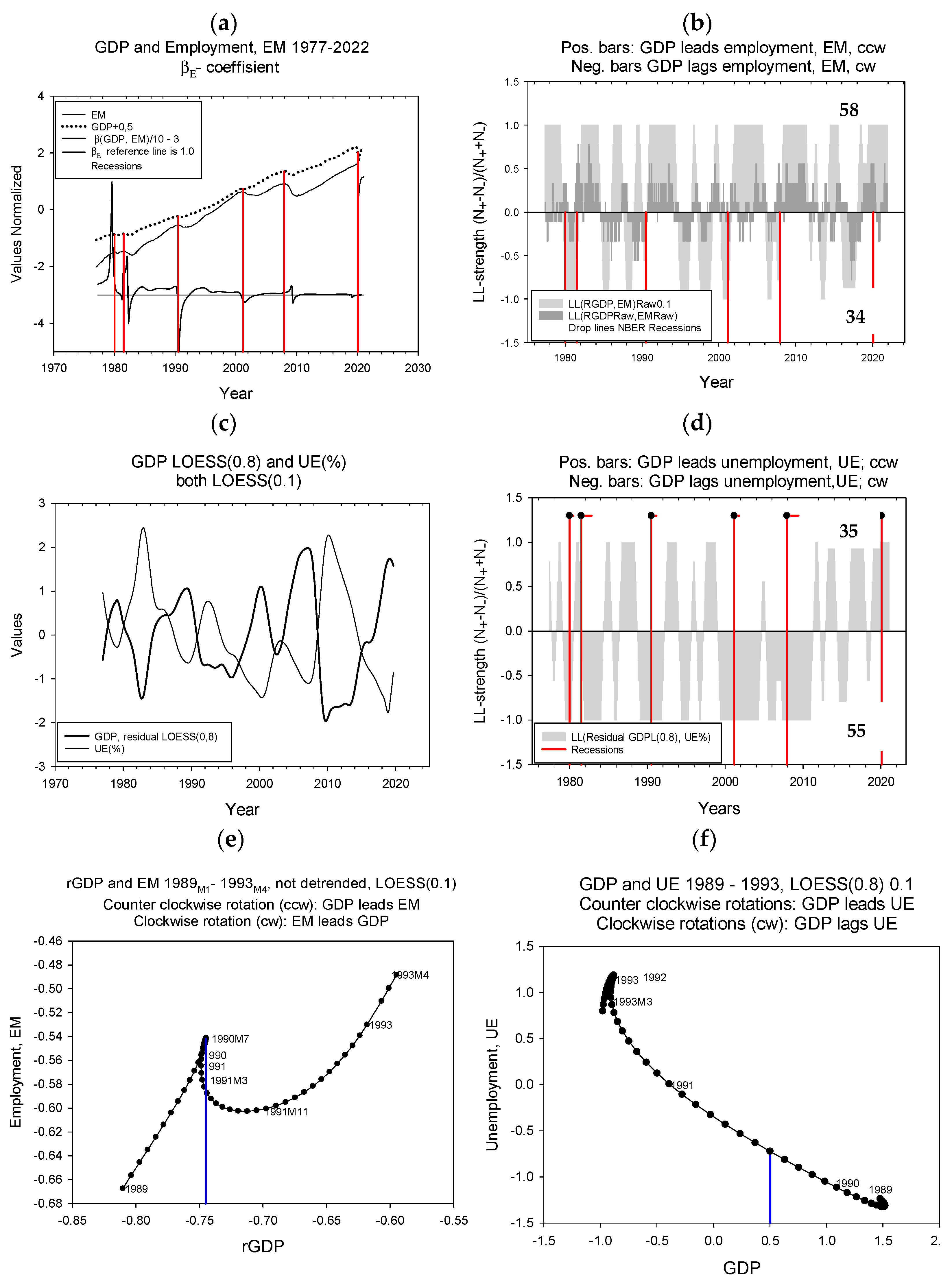
In Figure 2a, the upper two series show GDP and EM time series centered, normalized and slightly LOESS(0.1)-smoothed. The lower line shows the βE(9) coefficients for an OLR over a rolling 9-month time window. The βE coefficient shows characteristic peak anomalies for paired cyclic curves where one curve is sifted in time relative to the other. The droplines show when the NBER recessions starts. Figure 2b shows the LL relations for the GDP and EM series in Figure 2a. The dark grey bars show θ(3) and the light grey bars show LL(9). GDP leads EM pseudo-significantly 58% of the time and GDP leads EM pseudo-significantly 34% of the time. Table 1 shows the number of months during a 12-month period where θ(3) < 0. Figure 2c shows the residual time series for LOESS(0.8)-smoothed GDP. This series and the UE series are, in addition, slightly LOESS(0.1)-smoothed to avoid sharp peaks.
Figure 2d shows the LL relations between the two series. GDP leads UE pseudo-significantly 35% of the time and GDP lags UE pseudo-significantly 55% of the time. The LL(GDP,UE) relation shows that UE may lead GDP both before and after a recession.
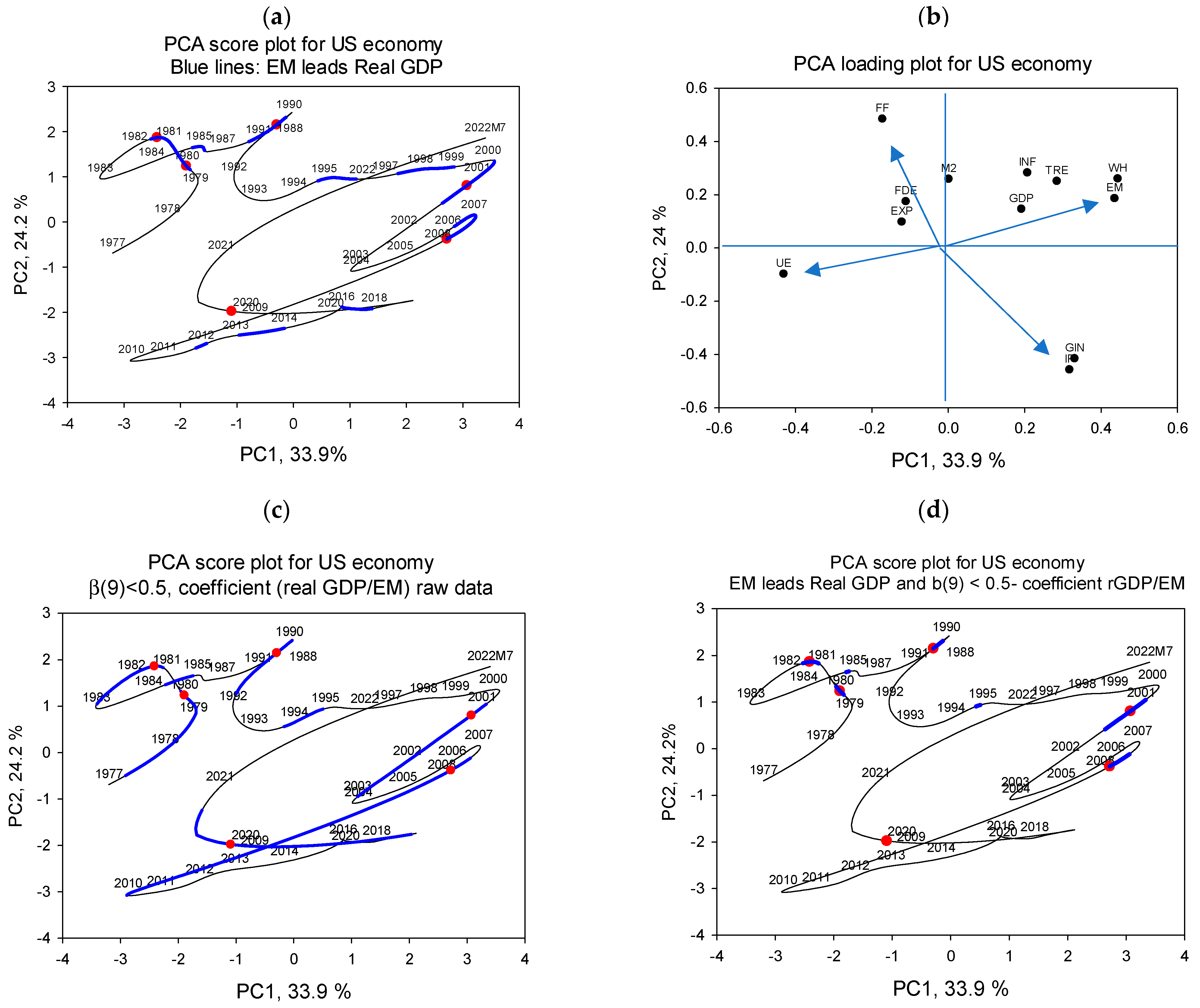
The LL relations for GDP and EM could in principle be the inverse of the LL relations for GDP and UE. To see how the differences would show up in a phase plot, we plotted the GDP/EM series and the GDP/UE series for time windows around the 1990 recession in two phase plots for the years 1989M1 to 1993M4 (Figure 2e,f). The drop lines show the timing of the July 1990 recession. The graph shows both associations and rotational directions. The results for the GDP/EM pair are shown embedded in a “map” of the US economy in Figure 3a. The blue lines show that the recessions, with the 2020 recession as an exception, are associated with a leading relation for EM to GDP (EM → GDP), but EM also leads GDP during other periods. Figure 2f shows that higher GDP generally leads to lower UE. However, there is no discontinuity around the 1990 recession as it was with the GDP/EM pair.

4.3. The βE Coefficient

The βE coefficients are calculations over 9 months. Figure 2a shows that the βE coefficient is generally greater than 1.0 before a recession and then becomes less than 1.0 for a period of 4 to 52 months (21 ± 17 months) after the recession. Table 1 shows the values of the βE coefficient when it has its lowest value around the recession periods. In Figure 3c, the result is embedded in the “map” of the US economy. The distribution of the blue lines suggests that the period with the βE coefficient less than 0.5 is mostly associated with recession periods. Figure 3d shows that time windows where both EM leads GDP and βE(9) is less than 0.5 are concentrated around the recessions. The 2020 recession is an exception.

4.4. US Economy Results

The “map” of the US economy seen in the loading plot on Figure 3b provides a reasonable stylized picture of an economy. There are some obvious relations. EM and UE point in opposite directions and align roughly with the x-axis. FF and IP point in opposite directions and align roughly with the y- axis. GDP, EM, WH and TRE all have high values at the same time. However, the close connection between IP and GIN may not be intuitive. A PCA loading plot of cyclic series will have some other characteristics relative to series with Gaussian distributions. If two identical and perfect sine functions are shifted a quarter of a cycle length (λ/4) relative to each other, their symbol representation will be connected to the origin with lines that are at 90o to each other (Seip and Grøn 2019). Thus, FF and EM may have similar cycle periods, but will be shifted λ/4 relative to each other.
Recessions appear to occur in all parts of the “map”, but they are appearing after sharp bends in the trajectories. For the 1980, 1981 and 1990 recessions, trajectories are counterclockwise, whereas the trajectories rotate clockwise for the 2000, 2007 and 2020 recessions. The two series showing that EM → bGDP and βE(9) < 0.5 coincide in 34 months out of 547 months (Figure 3d). The 34 months partly preceded and partly followed five of six NBER recession dates, providing a probability of ≈0.0002 to coincide with the recessions by chance.

4.5. Labor Productivity

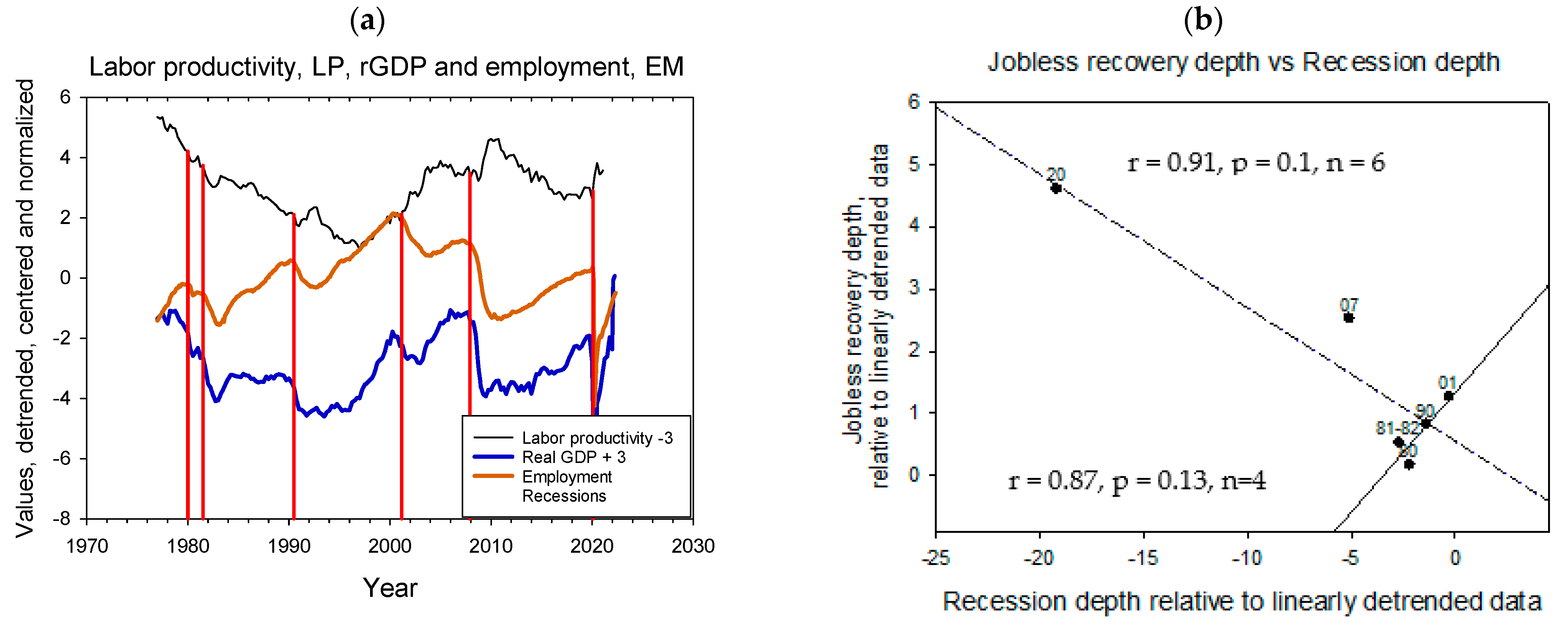
Labor productivity is generally regarded as a leading variable to the business cycle, (Abel et al. 1998, p. 321). Figure 4a and Table 1 show that the detrended LP is declining one year before most recessions, except the 2008 recession. On a decennial time scale, LP shows an overall decrease during the period 1977 to 1997 (the stagflation period under Volcker ≈ 1975–1985 and “the great moderation” period under Greenspan, ≈1985–1997, (McNown and Seip 2011) then increases until 2010 and decreases again until 2018. For the 12 months preceding a recession, the βE coefficient is zero per definition for linearly detrended series, but it is on average (minus) 0.10 ± 0.22, and all βE coefficients are either negative or close to zero. These values can be compared to the average 12-month increase of 0.28 in LP during the period 1996 to 2010.
We compared the five recession characteristics: recession depth and duration, LP depth and duration, and LP. However, we have only six sets of observation series, suggesting that outliers may play a dominant role. Figure 4b shows that outliers actually play a role for jobless recovery depth versus recession depth. Excluding the recessions in 2007 and 2020, it appears that jobless recovery depth is associated with recession depth, but the regression is not significant, and neither were the other five ((4 × 3/2) − 1) regressions.

5. Discussion

There is no firm conclusion about how the LL relations between GDP, UE or EM should be. However, changes in LL relations between GDP, UE and EM may be associated with the recession periods. Not all recessions are similar, and our study shows that the recent 2020 recession caused by the COVID-19 pandemic was different. The time window around a recession can been divided into four periods: first an expansion in GDP, then two periods during the downturn in GDP, and then a second expansion period where the economy recovers.
The first expansion is the one that triggers a monetary or financial response because the economy is overheating, e.g., a rise in FF (Taylor and Williams 2010). The first recession period is characterized by an uncertainty in the reality of the recession. During the third period, the recession is a certainty. The fourth period is the expansion period that terminates in “natural” growth and employment rates.

5.1. Lead-Lag Relations

A leading role for a causal effect is a prerequisite, but not a sufficient, criterion for causation. However, the leading role is often offered as a strong argument for a causal effect (Sugihara et al. 2012). We examined the LL relations between the two pairs: real GDP and EM, and GDP (detrended) and UE (percentages). Our results for EM support Hamilton’s (2018, p. 838) finding that the cyclical component of EM starts to decline before the NBER business cycle peak for essentially every recession (here, before 1981, 1990, 2001 and 2007 recessions). We also found that whereas EM leads GDP before a recession, it lags GDP after the recession.
Figure 2e,f showed two characteristics for paired time series during the period 1989 to 1993, that is, around the 1990 recession. The first shows how EM and UE vary with GDP (slopes in the graph), and it shows which of the variables are leading the others (rotational directions). The graphs confirm the LL—the results are in Figure 2b,d. In the following discussion, we use traditional “stylized facts” to explain the time series movements we observe. Following that, we will discuss possible causal factors examined in the literature.
Before July 1990M7, the first expansion, EM increases as GDP increases, and the rotational direction is clockwise (CW), but not easy to identify visually (Figure 2e). The graph confirms the LL results in Figure 2b. The interpretation could be that firms fill vacant positions as production or demand for services increases, but the overall US labor productivity anomaly decreases (from a linear trend) during the period one year before the 1990M7 recession. We did not find a first recession period where business was slow to cut workers. (Note that EM increases before 1990M1 (Figure 4a), whereas Figure 3a,b shows a movement towards higher UE at the same time). However, there are 12 variables in the PCA plot that show a movement towards a higher UE, so there are probably other variables that are responsible for the movement, e.g., working hours, as suggested by Obst (2020, p. 229) Following the trajectories in Figure 2e, it is seen that during the whole recession period from 1990M7, both GDP and EM decrease, but whereas GDP increases after March 1991M3, EM increases just slowly after November 1991M11 and is not up to pre-recession values before November 1992M11. Thus, for one year there is a “jobless recovery” during the second expansion period. During this expansion (the recovery), firms are slow to rehire as they use current workers more intensively. Rotations are counterclockwise, showing that GDP is leading EM from 1990M9 to 1993M4 (outside graph: to 1994M10). The labor production anomaly increases from 1991M1 to 1992M7. We have not discussed the effects of an increase in the underground economy during a recession, nor its potential impact on the recovery process. However, it may contribute a significant amount in countries with large underground economies, e.g., Seip and Orsi (2022).
For the GDP–UE pair (Figure 2f), GDP decreases and UE increases, rotations are clockwise, and UE leads GDP. However, it is the trough in unemployment that would imply a peak in GDP, thus, the interpretation should be that (minus) UE apparently leads GDP or GDP leads UE, i.e., it is business growth that creates hiring.
Our results are based on EM and UE data downloaded in September 2021, however Ahn and Hamilton (2022) conclude that current unemployment measures underestimate the number of people that are unemployed, and the magnitude of the bias is larger when the true unemployment rate is higher). Ahn and Hamilton (2022)’ s revised UE series running from 2001 to 2020 showed similar LL(GDP, UE) relations as in Figure 2d, except that from 2006 to 2010 GDP was leading UE. Mimicking the verbal Ahn and Hamilton assessments for the whole period of 1977 to 2020 and replacing UE with UE1.1, the results for the period did not change the LL(GDP, UE) patterns appreciably.
In contrast to the LL relations for GDP and EM, Elhorst and Emili (2022) found that for the Netherlands, output growth leads UE. However, the results reported here apply to employment and not to unemployment, and Figure 2e,f and Appendix A show that EM and UE provide different results when put into similar contexts.

5.2. The βE-Coefficient

We chose to calculate the βE coefficient over 9 months. Examining the phase plot for the period 1989M1 to 1992M10 in Figure 2e and following the βE(9) from left to right during the same time window in Figure 2a, the βE will first show a small positive peak, then after 1990 a sharp negative peak and last a horizontal “no change” trend.

5.3. LL-Relations and the βE-Coefficient

The following results apply to the five recessions during the period 1977 to 2010, but the COVID-19 recession in 2020 is an exception for all results. Figure 3d shows months where both EM leads GDP and the βE coefficient is less than 0.5, that is, less than the “neutral” slope of 1.0. This result support both our hypotheses. Hypothesis 1 (H1), that the EM leads GDP and EM decreases faster than GDP before and during a recession was supported. The NBER recessions come after sharp bends in the trajectories and away from optimal EM and GDP in Figure 3a (NBER recession dates are shown by red dots in Figure 3a–d). The leading relation for EM before a recession was also found by Hamilton (2018). Hypothesis 2, (H2), that GDP leads EM and βE (GDP/EM) decreases before and during an expansion, was also supported (Figure 2a,b). The COVID-19 recession in 2020 was, in contrast to the “classical economy overheating” recessions, initiated by the COVID-19 pandemic and caused at least partly by a supply side shock (Hobbs 2020).

5.4. US Economy

Jobless abatement measures: Hypothesis 3, (H3), that we could infer macroeconomic conditions where leading or lagging relations between EM and GDP were significant, was not supported. Changes in LL relations were closely associated with recessions but distributed over the whole economy “map”. However, the finding that the NBER recession dates come after a sharp bend in the trajectories describing the US economy in Figure 3 may offer some clues. Several studies suggest various factors that may explain variations in Okun’s β coefficient, such as changes in working hours and labor productivity (Cazes et al. 2013; Elhorst and Emili 2022), nominal wages, (Donayre and Panovska 2021 Okun’s beta and wages covary positively, p. 9), labor legislation, (Cazes et al. 2013) and a mismatch in job search (Mukoyama and Sahin 2009; Gimbel and Sinclair 2020). The selection of variables used to build the PCA plots was chosen primarily to construct and validate the score plot for the US economy. We were not able to extract reasonable information from the loading plot in Figure 3b that could be used to associate any of the variables with the “jobless recovery” issue.

5.5. Policy Implications

Observations. First, the leading relations of EM → GDP before five of the six recessions and the leading relation of GDP → EM after recessions provided clear signatures to the Okun’s βE(t) signature. Second, periods before recessions were associated with labor productivity that was less than optimal. Third, we found that months where both EM → GDP and Okun’s βE(GDP,EM) were less than 0.5 were closely associated with the five recessions before 2010. The COVID-19 recession in 2020 was an exception. Fourth, months that are common for the two events (34 months) precisely identify recessions, and fifth, jobless recoveries were pronounced for all five recessions.
Interpretations. Since EM leads GDP before a recession, it suggests that hiring is made before business increases. This is supported by a decrease, or slowing down, in labor productivity. During economic recovery, hiring is slower, providing a background for the term “jobless recovery”.
Diagnostics predictions and abatements. The 34 months where EM → GDP and βE < 0.5 matched the recessions, indicating that some of the months precede the recession. Thus, inspecting the two series: (i) LL relations between GDP and EM and (ii) Okun’s law in the format βE = GDP/EM, may help us to predict a recession or support that a recession is real. However, the COVID-19 recession in 2020 provided an important exception to this “rule”, perhaps due to the different nature of this atypical recession that was caused by a pandemic.
We could suggest two abatement measures for jobless recoveries. The first is that management should not hire workers during expansion periods that show a sign of a coming recessions. An assessment of the “natural” rise in labor productivity (the trend) is probably not easy to identify but examining labor productivity anomalies may still offer clues as to when new hirings should be made with care. The second measure is to implement legal procedures that make hiring and firing employees less easy. However, employment policy is a multicriteria question. The utility of being temporarily employed before a recession may be higher than the disutility of not being rehired for several months during a recession recovery (see, e.g., (Ball 2015)).
The results were not realized when EM was replaced by UE and real GDP by GDP. For a rationale, see Appendix A.

5.6. Further Studies

The present study addresses unemployment issues in terms of LL relations and OLR regressions between GDP/EM and time. Our results refer to the US economy, but a comparison with other countries along the same lines would be interesting, for example, comparing Okun’s βE(9) coefficient in the US with the corresponding βE(9) coefficients in Germany and the Netherlands. Volatilities in employment are largest in the US (0.0389), lower in the Netherlands (0.0232) and the lowest in Germany (0.0115).
We found that UE both leads and lags GDP, which would complicate shifting one series relative to the others to identify LL relations for the whole series (Figure 2d). For example, Obst (2020) includes two quarter delays between GDP and UE in analyzing the relation between GDP and UE. Figure A1a in Appendix A shows that even within time windows where the LL relations are consistent, cycle periods and phase shifts vary.
We also compared the two graphs GDP vs. UE (left in Figure A1) and GDP and EM (right in Figure A1), and it is seen that the graph for GDP and UE shows the overall “traditional” inverse relation between GDP and UE, whereas the GDP and EM graph does not directly reflect that UE and EM should be inverse measures of the same phenomenon. However, a contributing factor may be that if unemployed persons drop out of the labor force, they are no longer counted as unemployed in the unemployment statistics (Elhorst and Emili 2022). Thus, replacing UE with EM in Okun’s law appears to change the overall relation beyond the fact that the two variables EU and EM express inverse characteristics of labor participation. However, a discussion of these results is beyond the scope of the present study.

6. Conclusions

Loss of jobs is an important issue and optimum employment is among the three most important goals for the US federal reserve. Okun’s law, as expressed by its β coefficient, is traditionally formulated by the ratio between GDP and the UE gap, and over the whole period of study or for decennial time scales. Inspired by the results of Hamilton (2018), we replaced the normal measure of unemployment (UE) with employment (EM) and calculated a βE(9) = real GDP/EM. We found that EM became a leading variable to GDP before a recession, whereas GDP became a leading variable to EM after a recession. The shifts in the leading relation between GDP and EM around a recession also create peaks in the βE(9) coefficient around most “classical” recessions (the 2020 recession caused by the COVID-19 pandemic was an exception). All the recessions were also characterized by a decrease in labor productivity relative to an “optimal” but realized 1997–2010 value. Our findings of the leading role of EM to GDP before a recession and the loss in labor productivity suggest that hiring employees during periods with a heated economy may cause subsequent jobless recovery. To alleviate jobless recoveries, one should make hiring decisions with caution when there is a sign of a coming decision or labor productivity anomalies.

Author Contributions

Conceptualization, K.L.S., Methodology, K.L.S.; software, K.L.S.; validation K.L.S. and D.Z., Formal analysis, K.L.S. and D.Z., Investigation, K.L.S. and D.Z.; Resources, K.L.S. and D.Z.; Data curation, K.L.S. and D.Z.; Writing original draft, K.L.S. Review and Editing D.Z.; Visualization, K.L.S., Supervision, K.L.S. and D.Z.; Project administration, K.L.S. and D.Z.; calculations, K.L.S. and D.Z. All authors have read and agreed to the published version of the manuscript.

Funding

This research was funded by Oslo Metropolitan University.

Data Availability Statement

All data and all calculations are available from the author.

Conflicts of Interest

The author declare no conflict of interest.

Appendix A

The appendix contains: Comparing rGDP to EM and UE.

Comparing rGDP to EM and UE

The EM were significantly shifted 1.6 time steps backward relative to rGDP in 16*% of the time, and EM was significantly shifted forward 1.7 time steps relative to rGDP 33 % of the time.
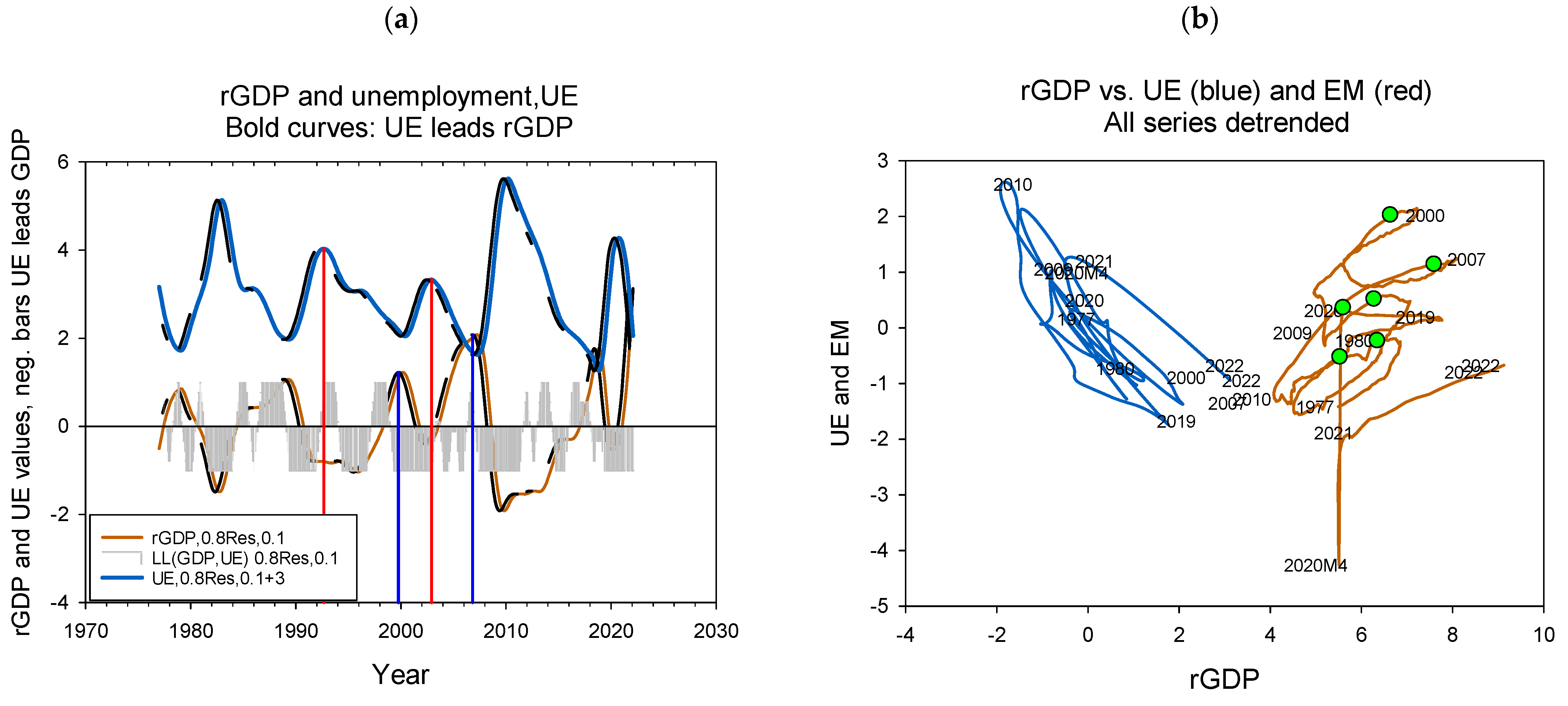
Figure A1. GDP and unemployment. (a) time series in bold shows part of the series where UE leads GDP. Distance between the two first peaks (red and blue dropdown lines) are 86 months and distance between the two next peaks are 47 months. (b) GDP versus UE and GDP versus EM. Green circles show NBER recessions.
Economies 10 00260 g0a1

References

  1. Abel, Andrew, Ben Bernanke, and Robert McNabb. 1998. Macroeconomics. Harlow: Addison-Wesley. [Google Scholar]
  2. Ahn, Hie Joo, and James D. Hamilton. 2022. Measuring labor-force participation and the incidence and duration of unemployment. Review of Economic Dynamics 44: 1–32. [Google Scholar] [CrossRef]
  3. Ball, Laurence. 2015. Monetary Policy for a High-Pressure Economy. Policy Futures. Washington: Center on Budget and Policy Priorities, p. 13. [Google Scholar]
  4. Burns, Arthur F., and Wesley C. Mitchell. 1946. Measuring Business Cycles. New York: National Bureau of Economic Research. [Google Scholar]
  5. Camacho, Maximo, and Gabriel Perez-Quiros. 2010. Introducing the Euro-Sting: Short-Term Indi-cator of Euro Area Growth. Journal of Applied Econometrics 25: 663–94. [Google Scholar] [CrossRef] [Green Version]
  6. Capsada-Munsech, Queralt, and Oscar Valiente. 2020. Sub-National Variation of Skill For-mation Regimes: A Comparative Analysis of Skill Mismatch Across 18 European Regions. European Education 52: 166–79. [Google Scholar] [CrossRef]
  7. Cazes, Sandrine, Sher Verick, and Fares Al Hussami. 2013. Why did unemployment respond so differently to the global financial crisis across countries? Insights from Okun’s Law. IZA Journal of Labor Policy 2: 1–18. [Google Scholar] [CrossRef] [Green Version]
  8. Donayre, Luiggi, and Irina Panovska. 2021. Recession-specific recoveries: L’s, U’s and everything in between. Economics Letters 209: 110145. [Google Scholar] [CrossRef]
  9. Elhorst, J. Paul, and Silvia Emili. 2022. A spatial econometric multivariate model of Okun’s law. Regional Science and Urban Economics 93: 103756. [Google Scholar] [CrossRef]
  10. Galí, Jordi, Frank Smets, and Rafael Wouters. 2012. Slow recoveries: A structural interpretation. Journal of Money, Credit and Banking 44: 9–30. [Google Scholar] [CrossRef] [Green Version]
  11. Gimbel, Martha E., and Tara M. Sinclair. 2020. Mismatch in Online Job Search. Paper presented at the LERA 2020 Meetings, Virtual, June 13–16; Sa Diego: Labor and Employment Relations Assocciation (LERA). [Google Scholar]
  12. Hamilton, James D. 2018. Why You Should Never Use the Hodrick-Prescott Filter. Review of Economics and Statistics 100: 831–43. [Google Scholar] [CrossRef]
  13. Hobbs, Jill E. 2020. Food supply chains during the COVID-19 pandemic. Canadian Journal of Agricultural Economics-Revue Canadienne D Agroeconomie 68: 171–76. [Google Scholar] [CrossRef] [Green Version]
  14. Krüger, J. Jens. 2021. A Wavelet Evaluation of Some Leading Business Cycle Indicators for the German Economy. Journal of Business Cycle Research 17: 203–319. [Google Scholar] [CrossRef]
  15. Lazear, Edward P., and James R. Spletzer. 2012. The United States Labor Market: Status quo or a New Normal? The Changing Policy Landscape. Jacson Hole: The Federal Reserve Bank of Kansas City. [Google Scholar]
  16. Maza, Adolfo. 2022. Regional Differences in Okun’s Law and Explanatory Factors: Some Insights from Europe. Interna-tional Regional Science Review 45: 016001762210823. [Google Scholar] [CrossRef]
  17. McNown, Robert, and Knut Lehre Seip. 2011. Periods and structural breaks in US economic history 1959–2007: A data driven identification. J. Policy Modelling 33: 169–82. [Google Scholar] [CrossRef]
  18. Mukoyama, Toshihiko, and Ayşegül Sahin. 2009. Why did the average duration of unemployment become so much longer? Journal of Monetary Economics 56: 200–9. [Google Scholar] [CrossRef] [Green Version]
  19. Obst, Thomas. 2020. Dynamic version of Okun’s law in the EU15 countries—The role of delays in the unemployment-output nexus. Scottish Journal of Political Economy 69: 225–41. [Google Scholar] [CrossRef]
  20. Seip, Knut L., and Hui Wang. 2022. The North Atlantic Oscillations: Lead–Lag Relations for the NAO, the AMO, and the AMOC—A High-Resolution Lead–Lag Analysis. Climate 10: 63. [Google Scholar] [CrossRef]
  21. Seip, Knut L., Øyvind Grøn, and Hui Wang. 2018. Carbon dioxide precedes temperature change during short-term pauses in multi-millennial palaeoclimate records. Palaeogeography Palaeoclimatology Palaeoecology 506: 101–11. [Google Scholar] [CrossRef]
  22. Seip, Knut L., Yunus Yilmaz, and Michael Schroder. 2019. Comparing Sentiment- and Behavioral-Based Leading Indexes for Industrial Production: When Does Each Fail? Economies 7: 104. [Google Scholar] [CrossRef] [Green Version]
  23. Seip, Knut L., and Øyvind Grøn. 2019. Atmospheric and Ocean Dynamics May Explain Cycles in Oceanic Oscillations. Climate 7: 77. [Google Scholar] [CrossRef] [Green Version]
  24. Seip, Knut Lehre, and Renzo Orsi. 2022. Effects of tax changes on GDP and underground economy: Italy 1982 to 2006. submitted. [Google Scholar]
  25. Søgner, Leopold. 2001. Okun’s law. Does the Austrian unemployment-GDP relationship exhibit structural breaks? Empirical Economics 26: 553–64. [Google Scholar] [CrossRef] [Green Version]
  26. Sugihara, George, Robert May, Hao Ye, Chih-hao Hsieh, Ethan Deyle, Michael Fogarty, and Stephan Munch. 2012. Detecting Causality in Complex Ecosystems. Science 338: 496–500. [Google Scholar] [CrossRef]
  27. Taylor, John B., and John C. Williams. 2010. Simple and Robust Rules for Monetary Policy. Working Papers. San Francisco: Federal Reserve Bank of San Francisco. [Google Scholar]
  28. Vaubel, Roland. 2008. The political economy of labor market regulation by the European Union. Review of International Organizations 3: 435–65. [Google Scholar] [CrossRef]
  29. Yellen, Janet L. 1991. Comments and discussion. Brookings Papers on Economic Activity 2: 127–33. [Google Scholar]
  30. Ziegenbein, Alexander. 2021. Macroeconomic shocks and Okun’s Law. Economic Letters 202: 1–4. [Google Scholar] [CrossRef]
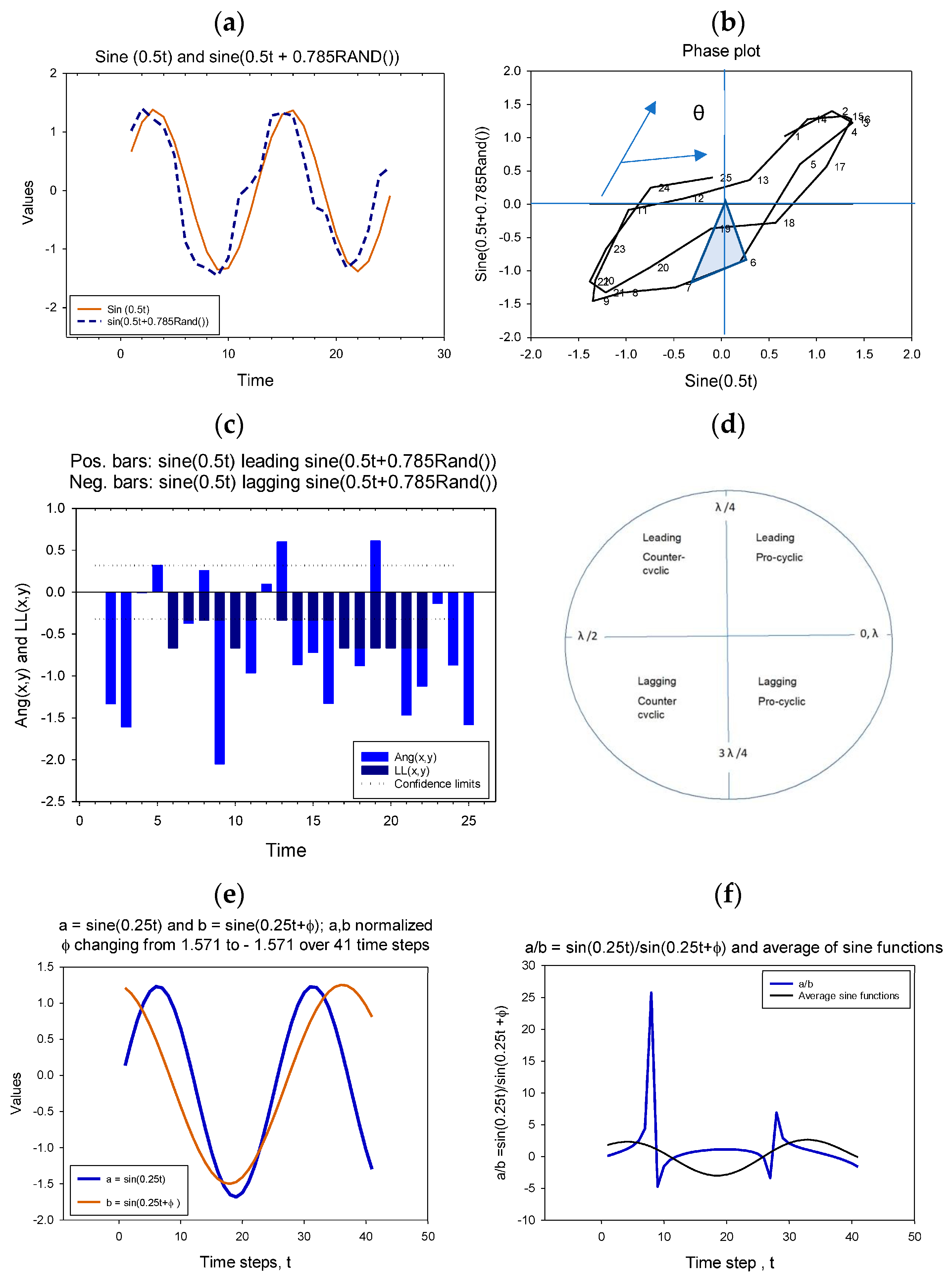
Figure 1. (a) Example: Calculating leading-lagging (LL) relations and LL-strength. Two sine functions: the smooth curve is a simple sine function, sin (0.5t), the dashed curve has the form sin (0.5t + ϕ × RAND()) where ϕ = +0.785 (b) In a phase plot with sin (0.5t) on the x-axis and the sin (0.5t + ϕ RAND()) on the y-axis, the time series rotates counterclockwise; θ is the angle between two consecutive trajectories. The wedge suggests the angle between the origin and lines to observations 6 and 7. (c) Angles between successive trajectories (light blue bars) and LL strength (dark blue bars). Dashed lines suggest confidence limits for persistent rotation in the phase plot and persistent leading or lagging relations in the time series plot. (d) LL relations and pro cyclic/counter cyclic relations between two cyclic series as a function of the phase shift between them. (e) Two sine functions; sin (0.25t + ϕ), the blue function has ϕ = 0 and the red function has ϕ shifted gradually from a positive to a negative value, thus the two functions shift in being a leading function. (f) The ratio a/b = sin (0.25t)/sin (0.25t + ϕ) as a function of time and the average of the two sine functions. (ad) are redrawn after Seip and Grøn (2019) and Seip and Wang (2022).
Economies 10 00260 g001
Figure 2. Lead-lag relations between GDP, employment (EM), and unemployment, (UE). (a) GDP and EM, both LOESS(0.1) smoothed. Drop lines show NBER recession. (b) LL relations between GDP and EM, both LOESS(0.1) smoothed (gray) and both raw, unsmoothed (dark gray). Numbers show percentage “pseudo significant” LL relations (see text). Drop-lines show the beginning of recessions. OLR between gray and black bars give R = 0.30, p < 0.001. (c) GDP-LOESS (0.8) residual and UE (%) both series LOESS(0.1) smoothed. (d) LL(GDP LOESS (0.8) residual, UE), both series LOESS(0.1) smoothed and normalized to unit standard deviation. Red horizontal lines show recession periods. Droplines show beginning of recessions. (e) Phase plot for GDP and EM, not detrended, 1989-1993M4, dropline show the beginning of the 1990 recession. (f) Same as (e), but with GDP and UE.
Economies 10 00260 g002
Figure 3. Principal component plots of US Economy 1977 to 2022. (a) Score plot for US economy. Blue lines show when employment leads real GDP: Red dots shows US NBER recessions. (b) Loading plot for US economy. (c) Same as a, but βE(9) < 0.5. See text. (d) same as (a), but both EM leads GDP and βE(9) < 0.5. UE = unemployment, FDE = federal debt, EXP = federal expenditures, FF = fed’s interest rate, M2 = monetary supply, M2, INF = inflation (we use the consumer price index), GDP = gross domestic product, TRE = tax receipts, GIN = Gini’s index, but reconstructed from Mukoyama and Sahin (2009), IP = industrial production, WH = working hours, EM = employment. βE(9) coefficient is for running GDP/EM.
Economies 10 00260 g003
Figure 4. Jobless recovery and recession depth. (a) Time series for linearly detrended labor productivity, GDP, and employment. Red droplines show recessions. (b) Jobless recovery depth as a function of recession depth. Separate regressions for all recessions and a subset where the two last recessions, 2007 and 2020, are excluded.
Economies 10 00260 g004
Table 1. Recessions in USA, 1977 to 2022. Beginning, end and duration are NBER data. GDP decline, labor productivity, jobless depth and jobless duration is measured as the anomaly from the linear detrended series.
BeginningEndDurationGDP Decline
(Peak to Trough)
EM Leads GDP before Recession (1)bE (GDP,EM) Coefficient PeaksbLP (LP,t) before Rec. (2)Jobless Depth (3)Jobless Duration (4)
MonthsRelative Values0–12 Months<0.50–12 Months Relative ValuesMonths
Jan 1980July 19806−2.23.00−0.30−0.041−0.1814
July 1981Nov 198216−2.712.000.18−0.022−0.5318
July 1990March 19918−1.45.00−0.160.000−0.8312
March 2001Nov 20018−0.311.00−0.64−0.010−1.2768 (5)
Dec 2007June 200918−5.19.000.480.019−2.54144 (5)
Feb 2020April 20202−19.21.00−0.1−0.015−4.6212
Average9.67 ± 5.40−5.15 ± 1.796.83 ± 3.87−0.25 ± 0.31−0.012 ± 0.020−1.66 ± 0.9144.67 ± 58.83
Number of months EM leads GDP during one years before a NBER recession. Peak value relative to a detrended βE. Deviation from linear trend. Months to pre-recession values. Employment does not recover to pre-recession values before next recession. Duration is the time between the two recessions.
Publisher’s Note: MDPI stays neutral with regard to jurisdictional claims in published maps and institutional affiliations.