Circuit Implementation of a Modified Chaotic System with Hyperbolic Sine Nonlinearities Using Bi-Color LED †

 ,
,  ,
, 
 and
and
Abstract
1. Introduction
2. The Proposed Chaotic Circuit
2.1. The Chaotic System of Differential Equations
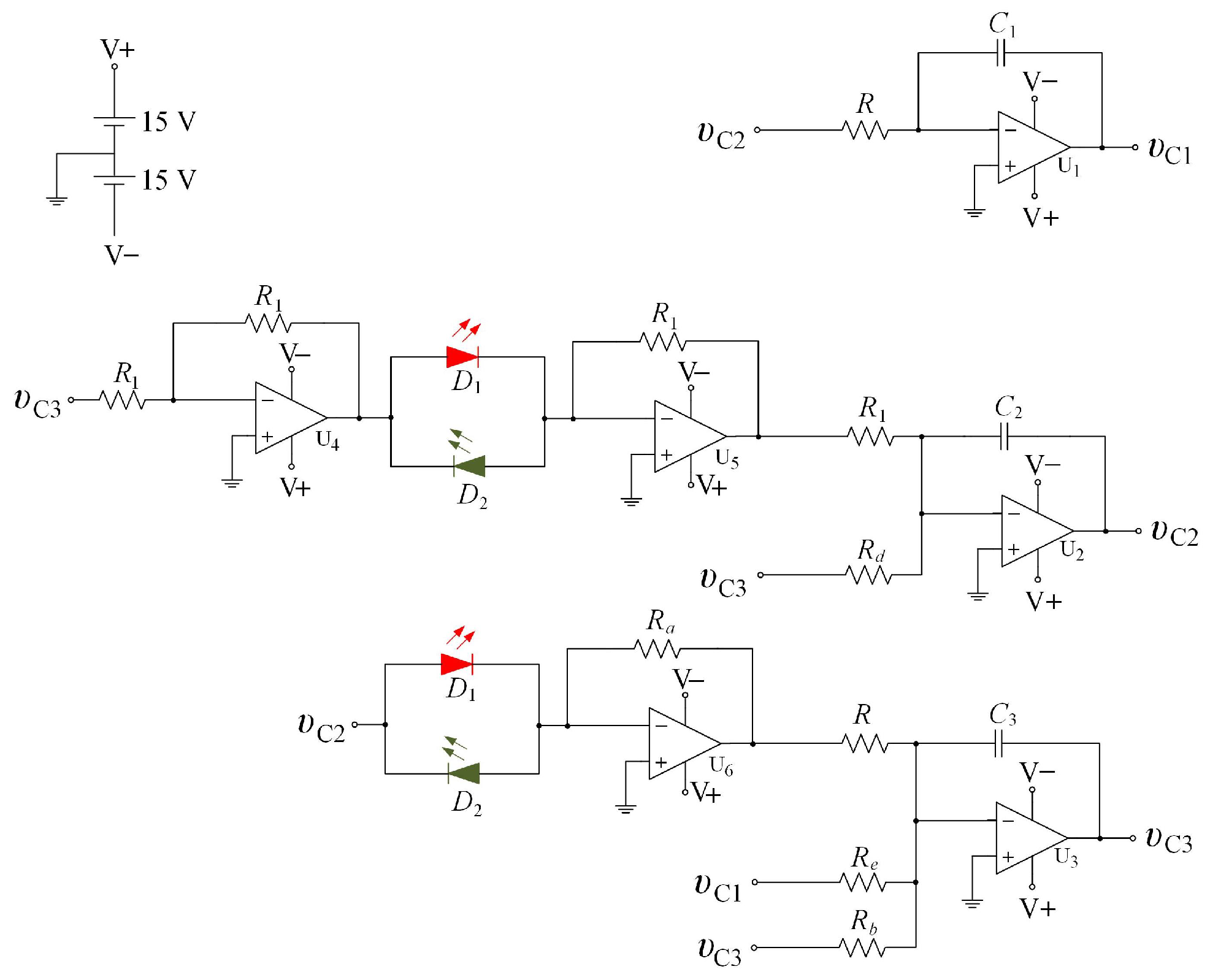
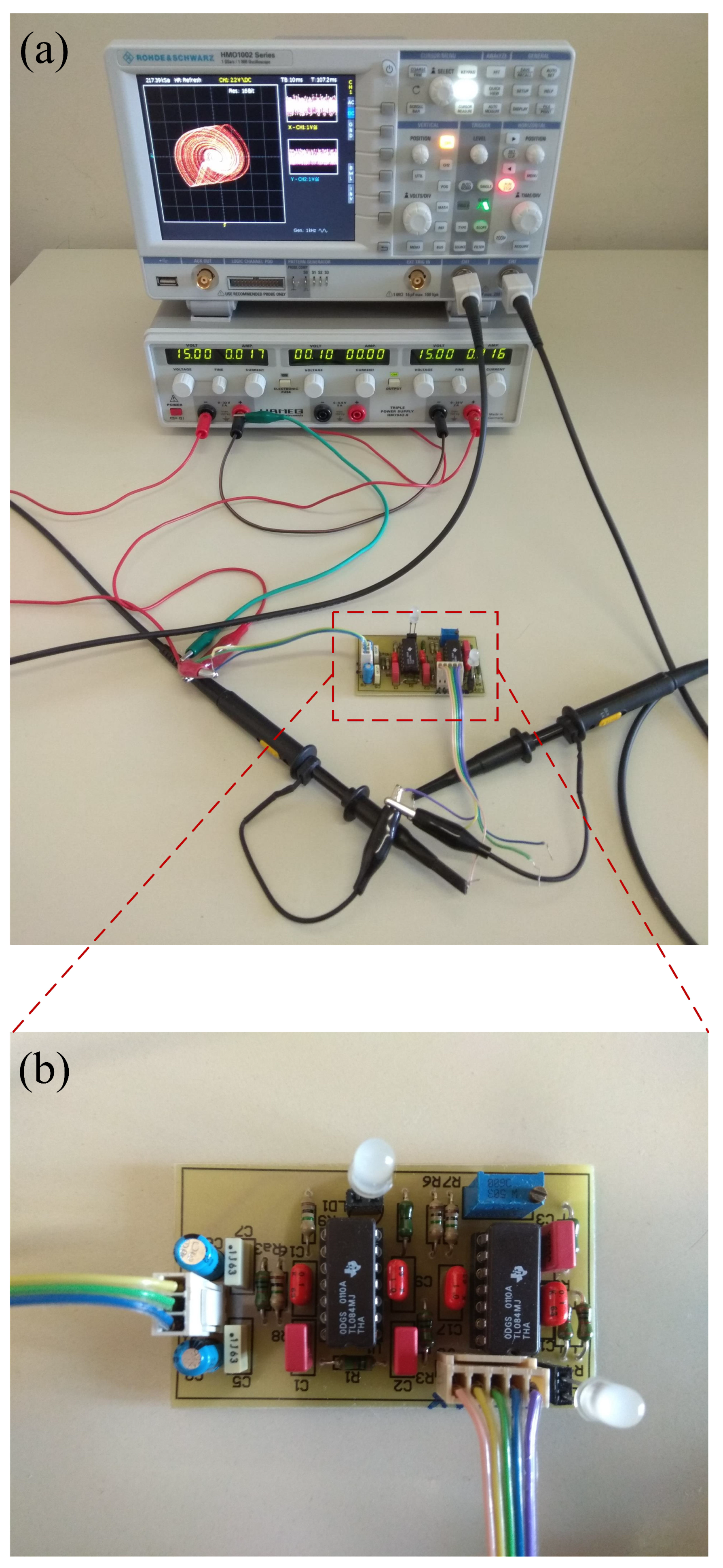
2.2. The Chaotic Circuit
3. Theoretical Study of The System
4. Circuit’s Dynamical Analysis
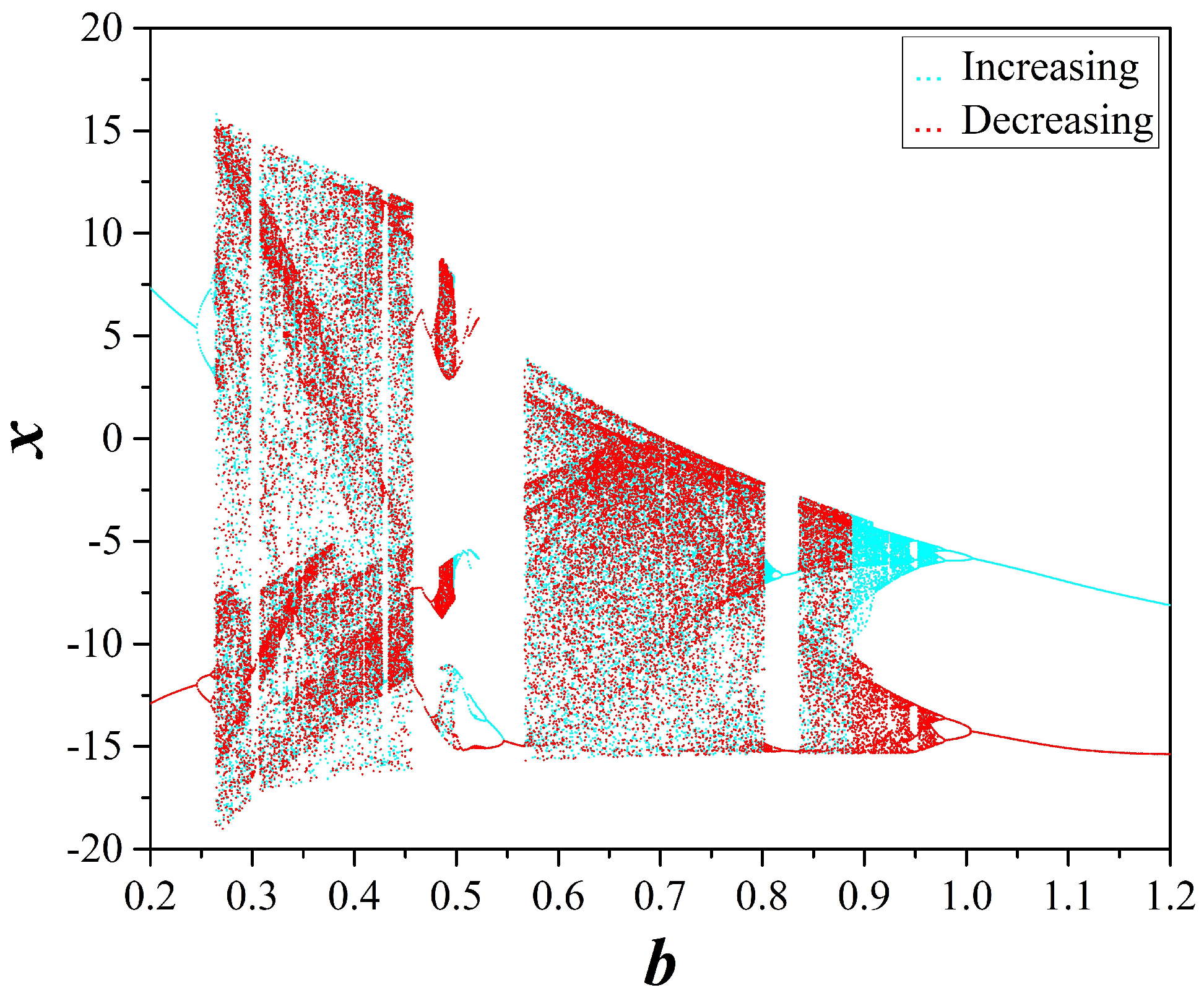
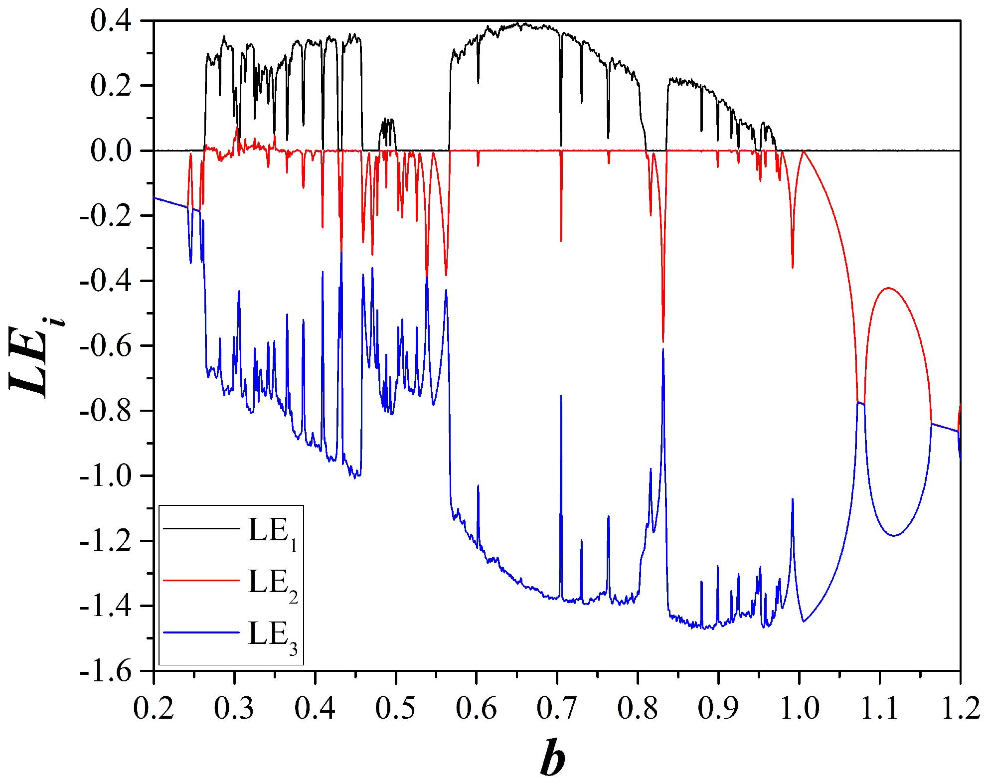
4.1. Dyncamical Behavior with Respect to b
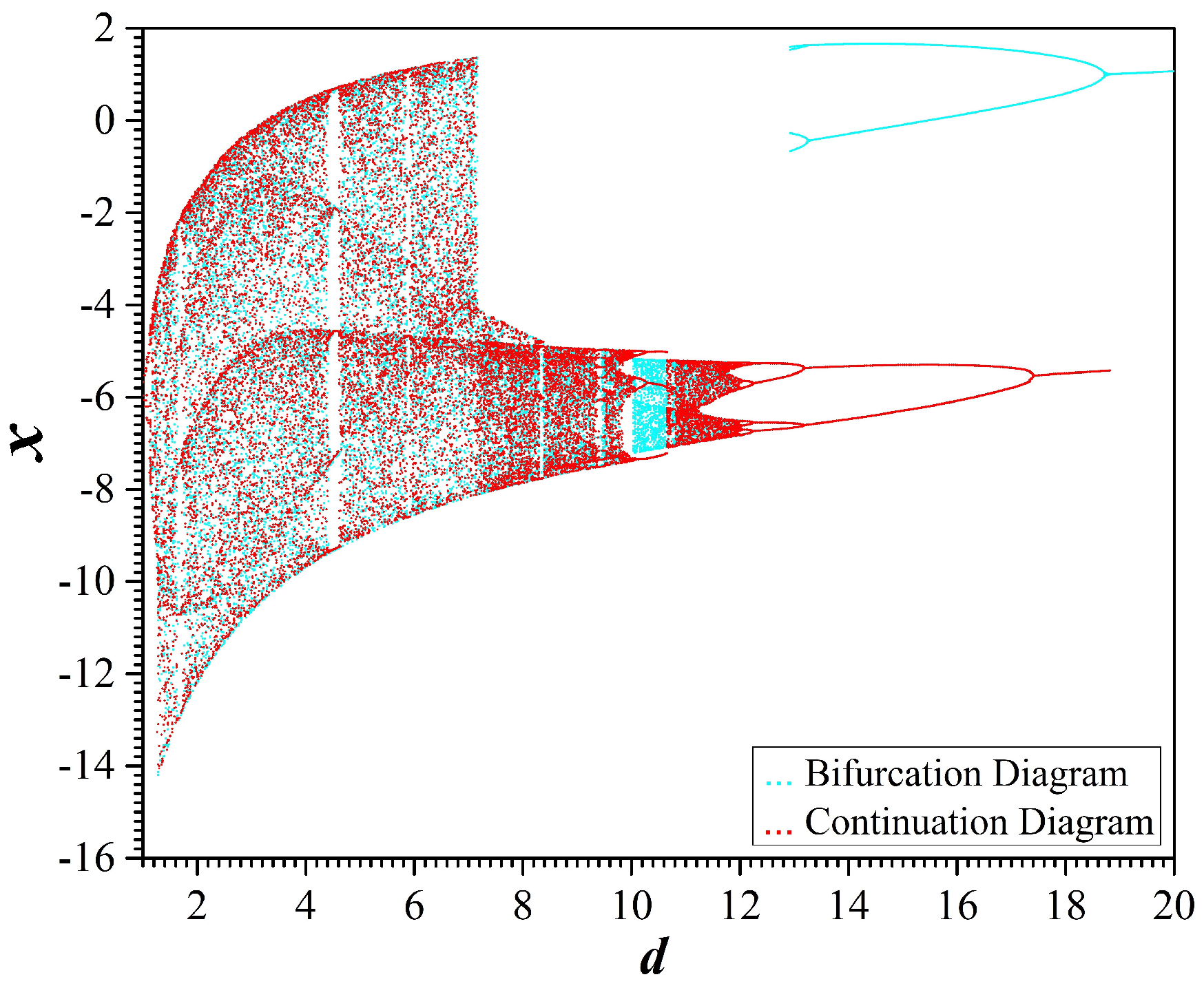
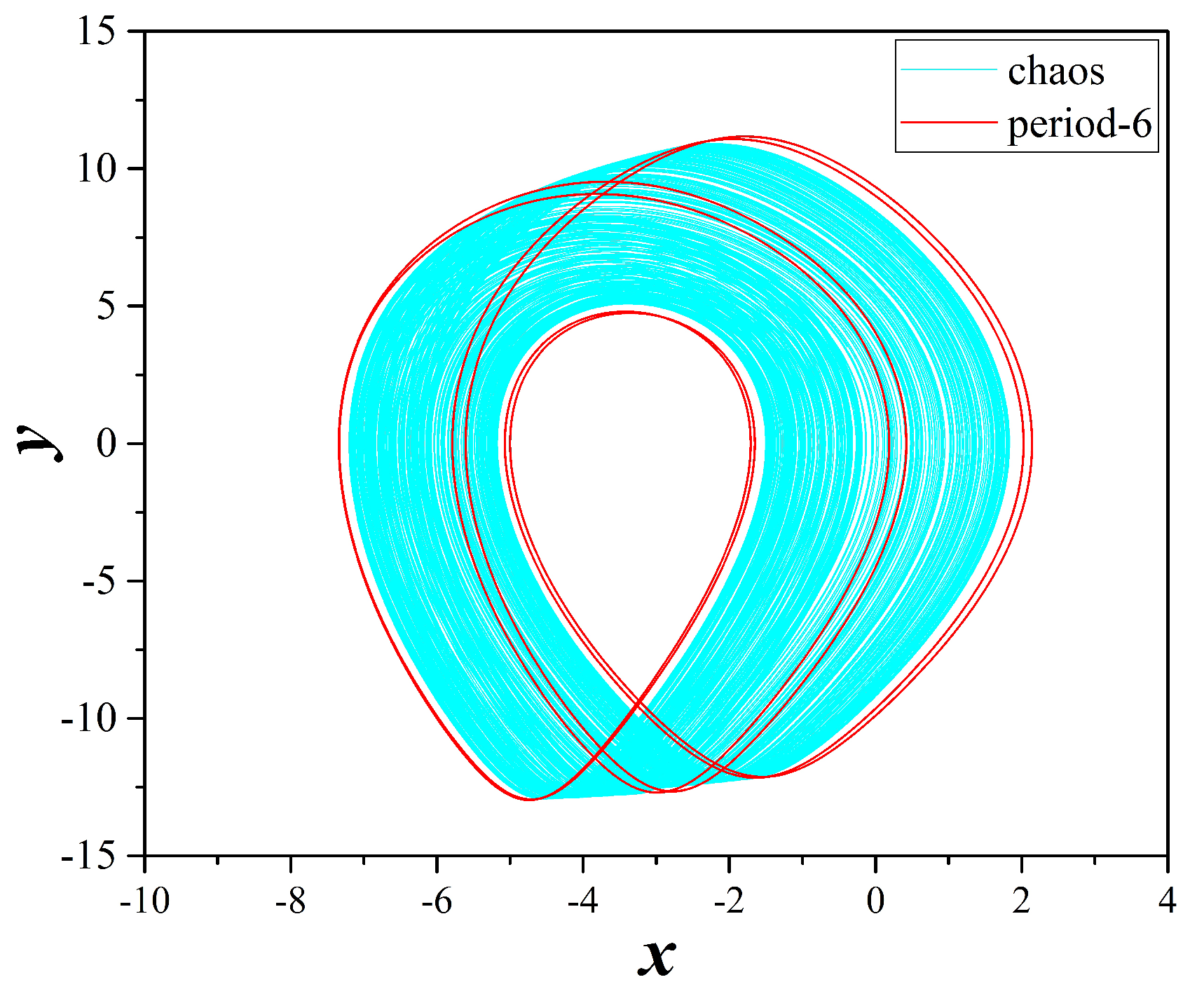
4.2. Dynamical Behavior with Respect to d
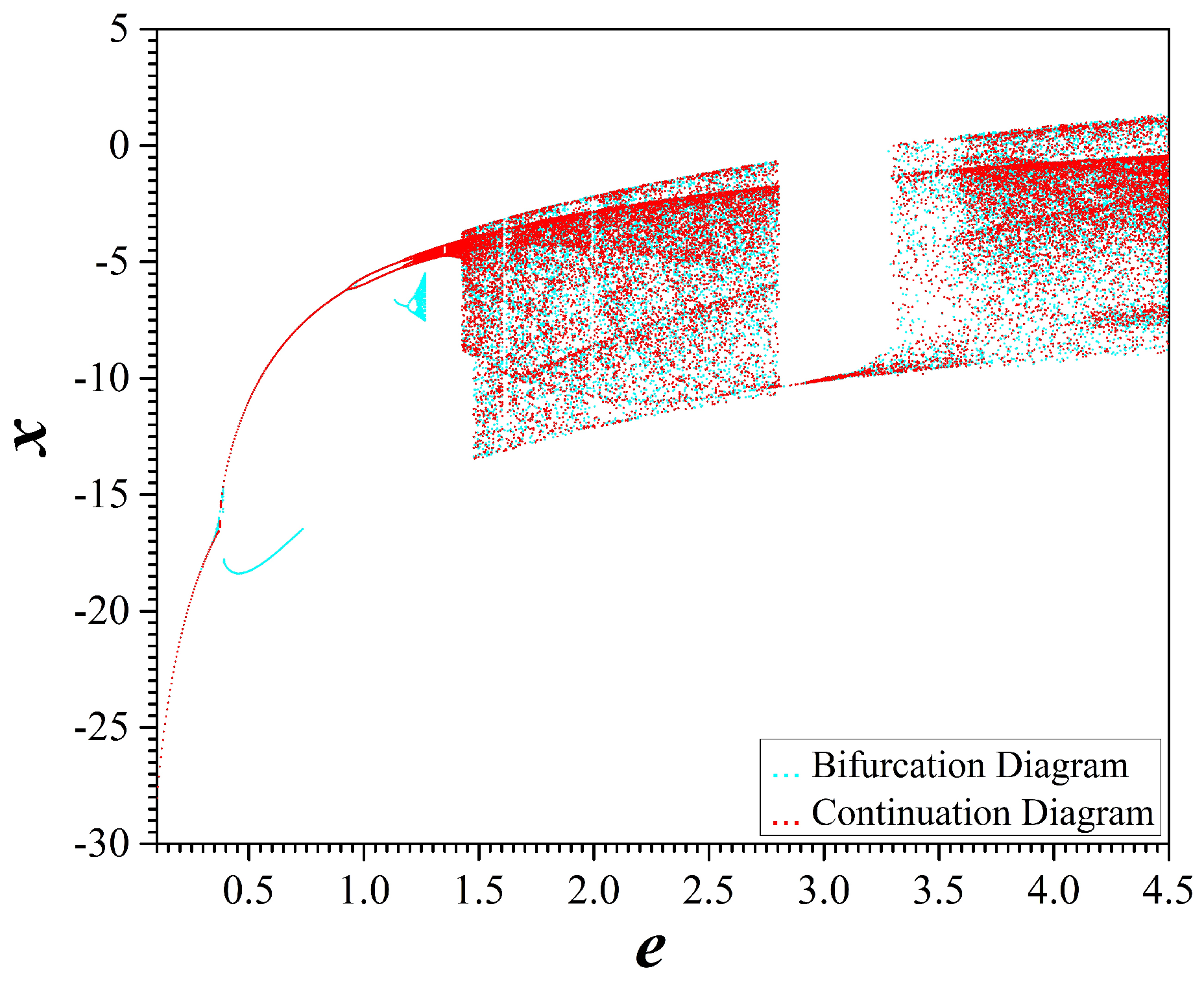
4.3. Dynamical Behavior with Respect to e
5. Conclusions
Author Contributions
Funding
Institutional Review Board Statement
Informed Consent Statement
Data Availability Statement
Conflicts of Interest
References
- Buscarino, A.; Fortuna, L.; Frasca, M.; Sciuto, G. A Concise Guide to Chaotic Electronic Circuits; Springer: Berlin/Heidelberg, Germany, 2014. [Google Scholar]
- Buscarino, A.; Fortuna, L.; Frasca, M. Essentials of Nonlinear Circuit Dynamics with MATLAB® and Laboratory Experiments; CRC Press: Boca Raton, FL, USA, 2017. [Google Scholar]
- Tlelo-Cuautle, E.; Pano-Azucena, A.D.; Guillén-Fernández, O.; Silva-Juárez, A. Analog/Digital Implementation of Fractional Order Chaotic Circuits and Applications; Springer: Berlin/Heidelberg, Germany, 2020. [Google Scholar]
- Kennedy, M.P. Chaos in the Colpitts oscillator. IEEE Trans. Circuits Syst. Fundam. Theory Appl. 1994, 41, 771–774. [Google Scholar] [CrossRef]
- Peter, K. Chaos in Hartley’s oscillator. Int. J. Bifurc. Chaos 2002, 12, 2229–2232. [Google Scholar] [CrossRef]
- Namajunas, A.; Tamasevicius, A. Modified Wien-bridge oscillator for chaos. Electron. Lett. 1995, 31, 335–336. [Google Scholar] [CrossRef]
- Chua, L.O. Chua’s circuit: An overview ten years later. J. Circuits Syst. Comput. 1994, 4, 117–159. [Google Scholar] [CrossRef]
- Li, C.; Thio, W.J.C.; Iu, H.H.C.; Lu, T. A memristive chaotic oscillator with increasing amplitude and frequency. IEEE Access 2018, 6, 12945–12950. [Google Scholar] [CrossRef]
- Kennedy, M.; Chua, L. Van der Pol and chaos. IEEE Trans. Circuits Syst. 1986, 33, 974–980. [Google Scholar] [CrossRef]
- Endo, T.; Chua, L.O. Chaos from phase-locked loops. IEEE Trans. Circuits Syst. 1988, 35, 987–1003. [Google Scholar] [CrossRef]
- Hamill, D.C.; Deane, J.H.; Jefferies, D.J. Modeling of chaotic DC-DC converters by iterated nonlinear mappings. IEEE Trans. Power Electron. 1992, 7, 25–36. [Google Scholar] [CrossRef]
- Kocarev, L.; Lian, S. Chaos-Based Cryptography: Theory, Algorithms and Applications; Springer: Berlin/Heidelberg, Germany, 2011; Volume 354. [Google Scholar]
- Yang, T. A survey of chaotic secure communication systems. Int. J. Comput. Cogn. 2004, 2, 81–130. [Google Scholar]
- Tsafack, N.; Kengne, J.; Abd-El-Atty, B.; Iliyasu, A.M.; Hirota, K.; Abd EL-Latif, A.A. Design and implementation of a simple dynamical 4-D chaotic circuit with applications in image encryption. Inf. Sci. 2020, 515, 191–217. [Google Scholar] [CrossRef]
- Yu, F.; Wang, C. A novel three dimension autonomous chaotic system with a quadratic exponential nonlinear term. Eng. Technol. Appl. Sci. Res. 2012, 2, 209–215. [Google Scholar] [CrossRef]
- Li, Y.; Huang, X.; Song, Y.; Lin, J. A new fourth-order memristive chaotic system and its generation. Int. J. Bifurc. Chaos 2015, 25, 1550151. [Google Scholar] [CrossRef]
- Lai, Q.; Chen, C.; Zhao, X.W.; Kengne, J.; Volos, C. Constructing chaotic system with multiple coexisting attractors. IEEE Access 2019, 7, 24051–24056. [Google Scholar] [CrossRef]
- Dalkiran, F.Y.; Sprott, J.C. Simple chaotic hyperjerk system. Int. J. Bifurc. Chaos 2016, 26, 1650189. [Google Scholar] [CrossRef]
- Pham, V.T.; Volos, C.; Jafari, S.; Vaidyanathan, S.; Kapitaniak, T.; Wang, X. A chaotic system with different families of hidden attractors. Int. J. Bifurc. Chaos 2016, 26, 1650139. [Google Scholar] [CrossRef]
- Zhang, G.; Zhang, F.; Liao, X.; Lin, D.; Zhou, P. On the dynamics of new 4D Lorenz-type chaos systems. Adv. Differ. Equ. 2017, 2017, 217. [Google Scholar] [CrossRef]
- Volos, C.; Akgul, A.; Pham, V.T.; Stouboulos, I.; Kyprianidis, I. A simple chaotic circuit with a hyperbolic sine function and its use in a sound encryption scheme. Nonlinear Dyn. 2017, 89, 1047–1061. [Google Scholar] [CrossRef]
- Pham, V.T.; Volos, C.; Kingni, S.T.; Kapitaniak, T.; Jafari, S. Bistable hidden attractors in a novel chaotic system with hyperbolic sine equilibrium. Circuits Syst. Signal Process. 2018, 37, 1028–1043. [Google Scholar] [CrossRef]
- Leutcho, G.; Kengne, J.; Kengne, L.K. Dynamical analysis of a novel autonomous 4-D hyperjerk circuit with hyperbolic sine nonlinearity: Chaos, antimonotonicity and a plethora of coexisting attractors. Chaos Solitons Fractals 2018, 107, 67–87. [Google Scholar] [CrossRef]
- Liu, J.; Sprott, J.C.; Wang, S.; Ma, Y. Simplest chaotic system with a hyperbolic sine and its applications in DCSK scheme. IET Commun. 2018, 12, 809–815. [Google Scholar] [CrossRef]
- Liu, J.; Ma, J.; Lian, J.; Chang, P.; Ma, Y. An approach for the generation of an nth-order chaotic system with hyperbolic sine. Entropy 2018, 20, 230. [Google Scholar] [CrossRef] [PubMed]
- Çavuşoğlu, Ü.; Panahi, S.; Akgül, A.; Jafari, S.; Kacar, S. A new chaotic system with hidden attractor and its engineering applications: Analog circuit realization and image encryption. Analog. Integr. Circuits Signal Process. 2019, 98, 85–99. [Google Scholar] [CrossRef]
- Giakoumis, A.; Androutsos, N.A.; Volos, C.K.; Moysis, L.; Nistazakis, H.E.; Tombras, G.S. A Chaotic Circuit with Bi-Color LED as a Nonlinear Element. In Proceedings of the 2020 9th International Conference on Modern Circuits and Systems Technologies (MOCAST), Bremen, Germany, 7–9 September 2020; pp. 1–4. [Google Scholar]
- Frederickson, P.; Kaplan, J.L.; Yorke, E.D.; Yorke, J.A. The Liapunov dimension of strange attractors. J. Differ. Equ. 1983, 49, 185–207. [Google Scholar] [CrossRef]
- Dawson, S.P.; Grebogi, C.; Yorke, J.A.; Kan, I.; Koçak, H. Antimonotonicity: Inevitable reversals of period-doubling cascades. Phys. Lett. A 1992, 162, 249–254. [Google Scholar] [CrossRef]
- Bao, H.; Hu, A.; Liu, W.; Bao, B. Hidden bursting firings and bifurcation mechanisms in memristive neuron model with threshold electromagnetic induction. IEEE Trans. Neural Netw. Learn. Syst. 2019, 31, 502–511. [Google Scholar] [CrossRef]
- Elwakil, A.S. Fractional-order circuits and systems: An emerging interdisciplinary research area. IEEE Circuits Syst. Mag. 2010, 10, 40–50. [Google Scholar] [CrossRef]


| Value of Parameter d | Behavior from the Bifurcation Diagram | Behavior from the Continuation Diagram |
|---|---|---|
| 10.1 | Chaos | Period-6 |
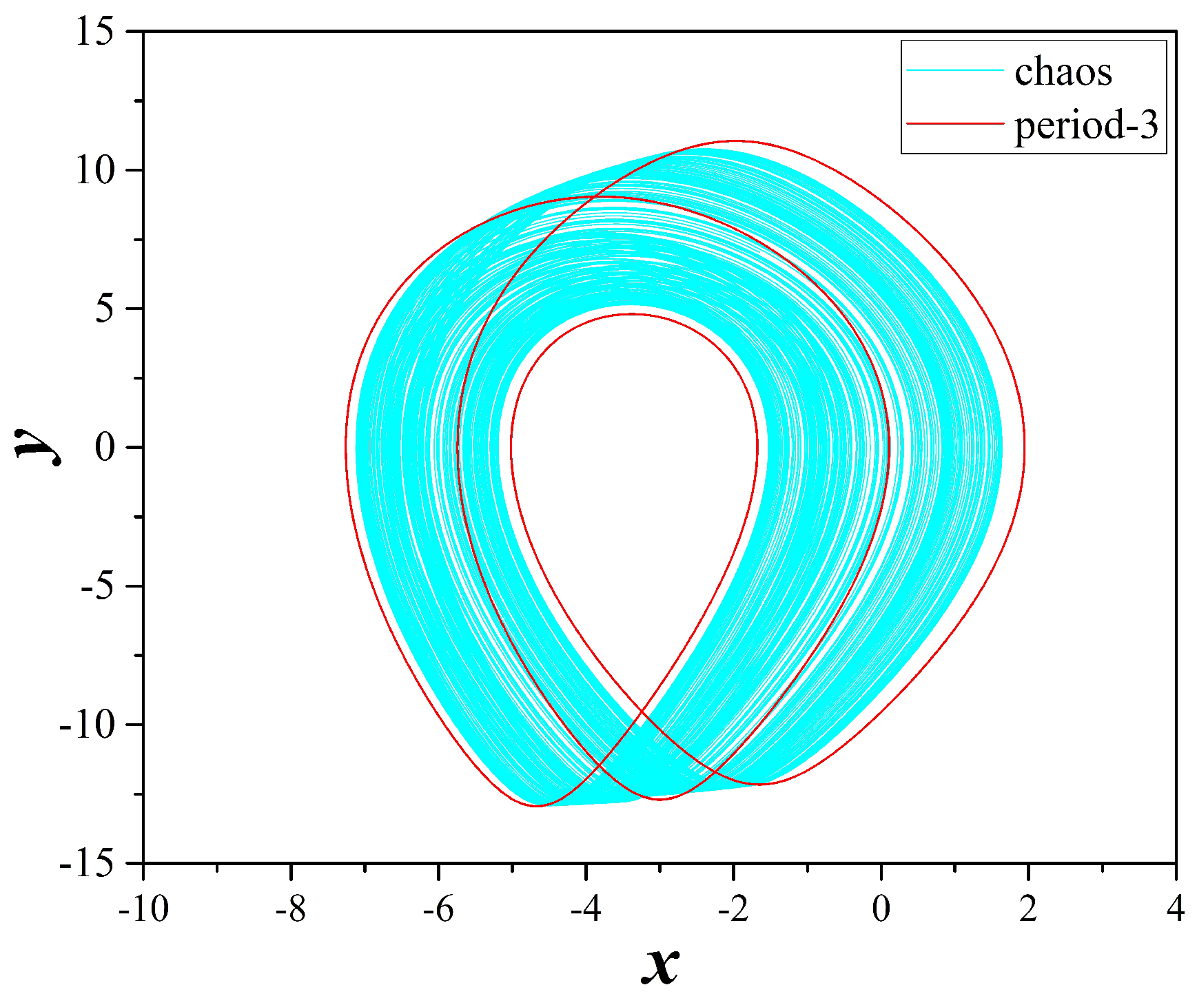
| 10.5 | Chaos | Period-3 |
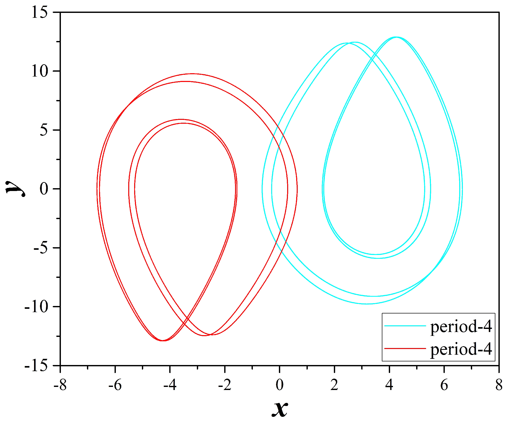
| 13.0 | Period-4 | Period-4 (symmetric) |
| 15.0 | Period-2 | Period-2 (symmetric) |
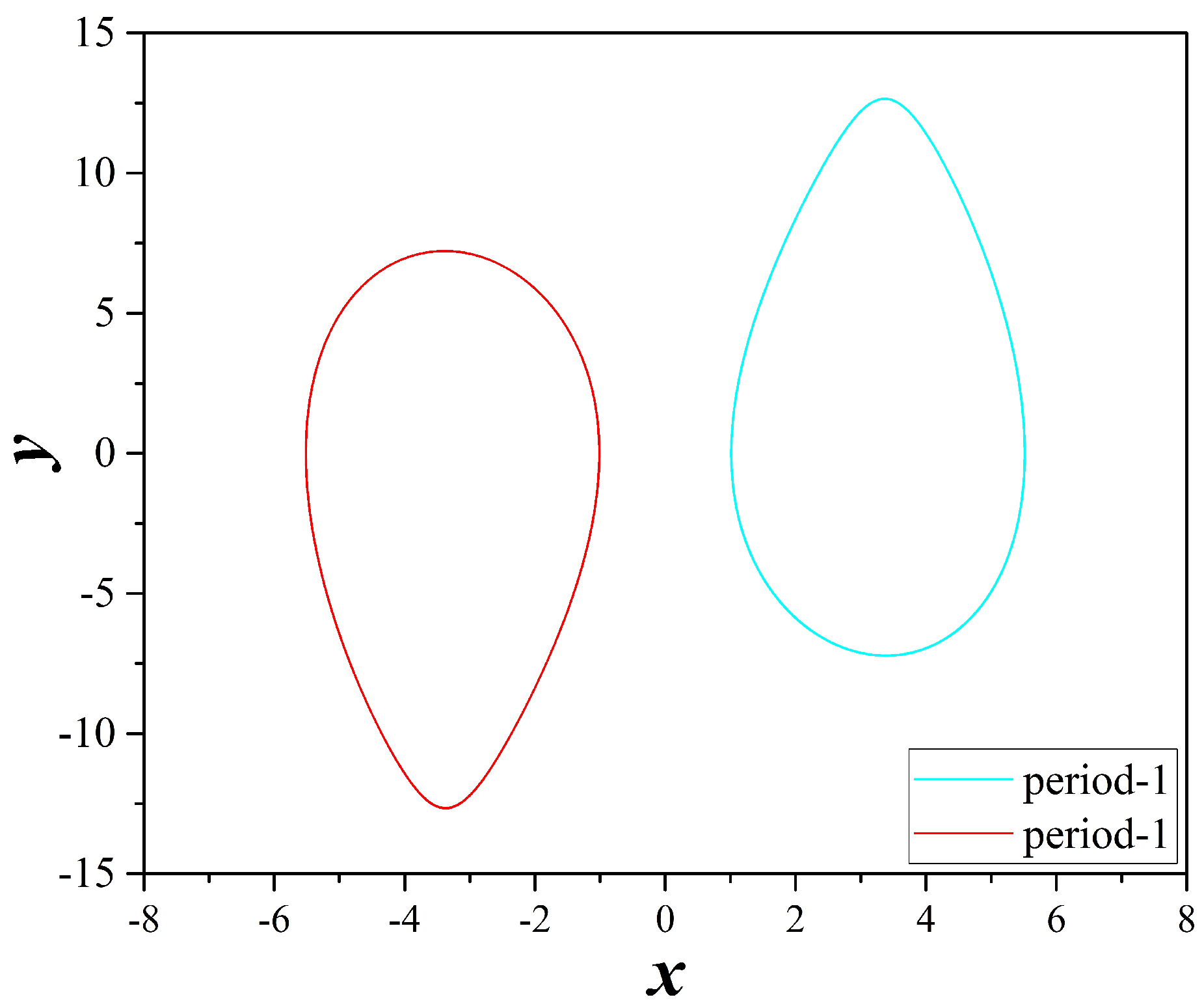
| 19.0 | Period-1 | Period-1 (symmetric) |
| Value of Parameter e | Behavior from the Bifurcation Diagram | Behavior from the Continuation Diagram |
|---|---|---|
| 0.50 | Period-1 | Period-1 (symmetric) |
| 1.15 | Period-1 | Period-2 |
| 1.20 | Period-2 | Period-4 |
| 1.26 | Chaos | Chaos (symmetric) |
Publisher’s Note: MDPI stays neutral with regard to jurisdictional claims in published maps and institutional affiliations. |
© 2021 by the authors. Licensee MDPI, Basel, Switzerland. This article is an open access article distributed under the terms and conditions of the Creative Commons Attribution (CC BY) license (http://creativecommons.org/licenses/by/4.0/).
Share and Cite
Volos, C.K.; Moysis, L.; Roumelas, G.D.; Giakoumis, A.; Nistazakis, H.E.; Tombras, G.S. Circuit Implementation of a Modified Chaotic System with Hyperbolic Sine Nonlinearities Using Bi-Color LED. Technologies 2021, 9, 15. https://doi.org/10.3390/technologies9010015
Volos CK, Moysis L, Roumelas GD, Giakoumis A, Nistazakis HE, Tombras GS. Circuit Implementation of a Modified Chaotic System with Hyperbolic Sine Nonlinearities Using Bi-Color LED. Technologies. 2021; 9(1):15. https://doi.org/10.3390/technologies9010015
Chicago/Turabian StyleVolos, Christos K., Lazaros Moysis, George D. Roumelas, Aggelos Giakoumis, Hector E. Nistazakis, and George S. Tombras. 2021. "Circuit Implementation of a Modified Chaotic System with Hyperbolic Sine Nonlinearities Using Bi-Color LED" Technologies 9, no. 1: 15. https://doi.org/10.3390/technologies9010015
APA StyleVolos, C. K., Moysis, L., Roumelas, G. D., Giakoumis, A., Nistazakis, H. E., & Tombras, G. S. (2021). Circuit Implementation of a Modified Chaotic System with Hyperbolic Sine Nonlinearities Using Bi-Color LED. Technologies, 9(1), 15. https://doi.org/10.3390/technologies9010015