The Importance of Introducing the OCTC Method to Undergraduate Students as a Tool for Circuit Analysis and Amplifier Design


 ,
, 

Abstract
:1. Introduction
2. Materials and Methods
2.1. OCTC Method
2.1.1. OCTC Principles
2.1.2. Applying the Method
- Select the i-th capacitor, , and remove all others. All decoupling and AC-coupling capacitors should be short-circuited.
- Set all independent sources to zero (i.e, short-circuit all independent voltage sources and open-circuit all independent current sources).
- Find the resistance seen by the ith capacitor. This can be done either by inspection or by replacing with a test current source , determining the voltage at its terminals, and calculating , (or, equivalently, by applying a voltage source and finding the current drawn from it).
- Repeat steps 1–3 for .
- Calculate T using (4).
- Calculate the dB frequency using (5).
2.2. Useful Analysis Tools
2.2.1. Small-Signal Equivalent Circuit—A Frequent Form
2.2.2. Miller Effect
2.2.3. Knowledge of Basic Amplifier Stages
2.3. Teaching Examples
- Collector–base junction capacitance
- Emitter–base junction capacitancewhere and .
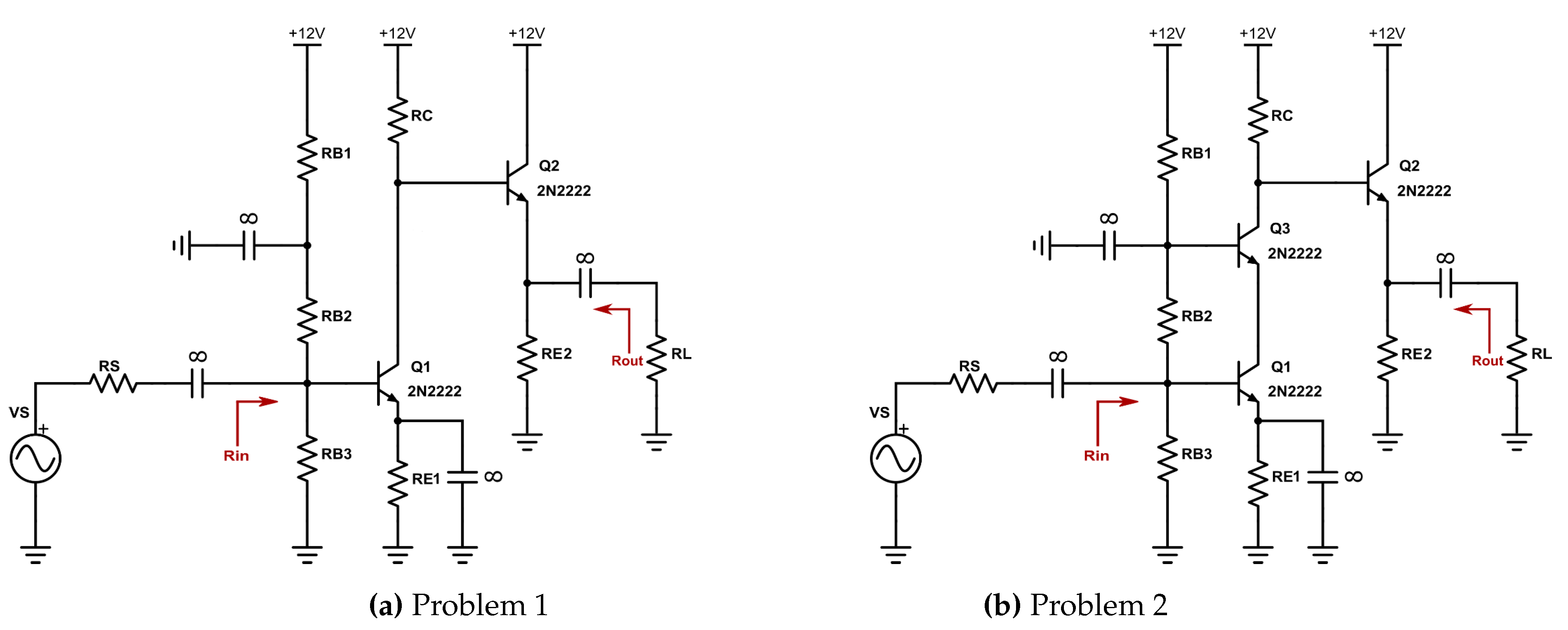
2.3.1. Problem 1
- Find (try to answer) directly what impedance every node “can see” (without drawing an AC equivalent circuit).
- For the BJT 2N2222 assume: , , , , , . Ignore the Early phenomenon (). Applying the OCTC method estimate the high 3dB frequency and so the bandwidth of the amplifier.
- Using LTspice for circuit simulation, sketch the Bode plot of the amplifier for the frequency range from to . Determine the high 3dB frequency and so the bandwidth of the amplifier.
2.3.2. Problem 2
2.3.3. Solutions and Simulations
2.4. Student Misconceptions
- Miller effect and open circuit time constant (OCTC) method. Students have difficulties recognizing and applying the Miller effect for a capacitance.
- Some students believe that the largest capacitor of the (transistors’ capacitances) has the greatest contribution in defining the upper cutoff frequency.
- Coupling and bypass capacitors in OCTC method. “Why don’t coupling and bypass capacitors contribute to the definition of the amplifiers’ upper cutoff frequency?” is the basic question. OCTC method approximately defines the upper cutoff frequency of an amplifier. It is used for high-frequency response of an amplifier. Upper and lower cutoff frequencies that define the bandwidth of an amplifier are often of greater interest than the complete transfer function. Coupling and bypass capacitors determine the lower cutoff frequency, whereas transistor (and stray) capacitances determine the upper cutoff frequency. Coupling and bypass capacitors are relatively large in value and their large impedances at high frequencies can be neglected. Thus coupling and bypass capacitors determine an amplifier’s low-frequency response. Transistor capacitances are relatively small in value and their large impedances at low frequencies can be neglected.
- What do we mean by “capacitors can be ignored”? Ignoring capacitors means that we operate at either a high enough or at a low enough frequency such that capacitors become either open or short circuits, leading to a “resistive” circuit. Note that the circuit is modified by the presence of the capacitors (e.g., elements may be shorted out). Capacitors typically divide into two groups: low-f capacitors (setting ) and high-f capacitors (setting ). We need to identify low-f and high-f caps. We will use absolute limits of (all capacitors open) and (all capacitors short) for this purpose.
- The role of bias circuits. For DC bias () all caps are considered as an open circuit.
- Non-symmetrical differential amplifiers. For a symmetric circuit, differential and common-mode analysis can be performed using “half-circuits”. Using “half-circuits” works only if the circuit is symmetric. Not all difference amplifiers are symmetric. Look at the load carefully. We can still use the “half-circuit” concept if the deviation from perfect symmetry is small. However, we need to solve both half-circuits.
2.5. A Sampling Test
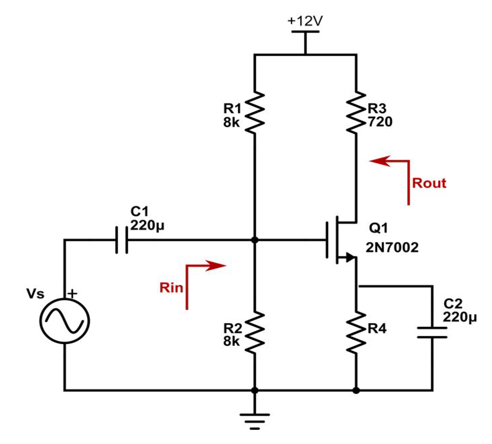
- Question 1: the MOS amplifier circuit displayed in Figure 3 is given. What is the computation relation, according to the circuit elements, of ?
- Question 2: the equivalent signal circuit of a two stage BJT amplifier, displayed in Figure 4a is given:
- (a)
- Find .
- (b)
- Which of the capacitances , , and do you think has the greatest impact on limiting the amplifier bandwidth and why?
- (c)
- What circuit modification can you propose to reduce the impact of the capacitance you selected in question (c)?
3. Results
3.1. Students’ Performance—Homework Problems
3.2. Students’ Performance—Sampling Test
3.3. Students’ Performance—Final Exam
3.4. Quantitative Evaluation
- Q[1.1] The course will increase my affinity to OCTC method.
- Q[1.2] I am interested in the course.
- Q[1.3] The effort imposed by the course is worthwhile because of the abilities and knowledge that I will acquire.
- Q[1.4] The use of simulation tools will increase my affinity to the OCTC method.
- Q[1.5] The use of simulation tools will help me to improve my academic results.
- Q[2.1] The course has increased my affinity to the OCTC method.
- Q[2.2] The course was interesting.
- Q[2.3] The effort imposed by the course was worthwhile because of the abilities and knowledge acquired.
- Q[2.4] The use of simulation tools increased my affinity to OCTC method
- Q[2.5] The use of simulation tools has helped me improve my academic results.
4. Discussion
5. Conclusions
Author Contributions
Funding
Conflicts of Interest
Appendix A. Academic Year in Greece
References
- Mulligan, J. The Effect of Pole and Zero Locations on the Transient Response of Linear Dynamic Systems. Proc. IRE 1949, 37, 516–529. [Google Scholar] [CrossRef]
- Thornton, R.D. Multistage Transistor Circuits; John Wiley & Sons, Inc.: Hoboken, NJ, USA, 1965. [Google Scholar]
- Voudoukis, N.F.; Baxevanakis, D.; Papafotis, K.; Dimas, C.; Oustoglou, C.; Sotiriadis, P.P. Introducing Senior Undergraduate Students to the Open-Circuit Time-Constant Method for Circuit Analysis. In Proceedings of the 8th International Conference on Modern Circuits and Systems Technologies (MOCAST), Thessaloniki, Greece, 13–15 May 2019. [Google Scholar] [CrossRef]
- Gray, P.R.; Hurst, P.J.; Lewis, S.H. Analysis and Design of Analog Integrated Circuits, 5th ed.; WILEY: Hoboken, NJ, USA, 2009. [Google Scholar]
- Sedra, A.S.; Smith, K.C. Microelectronic Circuits, 5th ed.; Oxford University Press: Oxford, UK, 2004. [Google Scholar]
- Sotiriadis, P.P. Lecture Notes on Electronics III; National Technical University of Athens: Athens, Greece, 2019. [Google Scholar]
- Salvatori, S.; Conte, G. On the SCTC-OCTC Method for the Analysis and Design of Circuits. IEEE Trans. Educ. 2009, 52, 318–327. [Google Scholar] [CrossRef]
- Pagiatakis, G.; Voudoukis, N. Operational amplifiers teaching and students’ understanding. In Proceedings of the 2017 IEEE Global Engineering Education Conference (EDUCON), Athens, Greece, 26–28 April 2017. [Google Scholar] [CrossRef]
- Voudoukis, N.; Pagiatakis, G. Students’ misconceptions in telecommunications. In Proceedings of the ISNITE2015 International Symposium, Volos, Greece, 11–13 September 2015. [Google Scholar]
- Tortoreli, M.D.; Chatzarakis, G.E.; Voudoukis, N.F.; Pagiatakis, G.K.; Papadakis, A.E. Teaching fundamentals of photovoltaic array performance with simulation tools. Int. J. Electrical Eng. Educ. 2016, 54, 82–94. [Google Scholar] [CrossRef]
- Macias-Guarasa, J.; Montero, J.; San-Segundo, R.; Araujo, A.; Nieto-Taladriz, O. A Project-Based Learning Approach to Design Electronic Systems Curricula. IEEE Trans. Educ. 2006, 49, 389–397. [Google Scholar] [CrossRef]
- Assaad, R.S.; Silva-Martinez, J. A Graphical Approach to Teaching Amplifier Design at the Undergraduate Level. IEEE Trans. Educ. 2009, 52, 39–45. [Google Scholar] [CrossRef]
- Pigazo, A.; Moreno, V.M.; Estebanez, E.J. An experience on e-learning in renewable energy: design and control of photovoltaic plants. In Proceedings of the 2009 3rd IEEE International Conference on E-Learning in Industrial Electronics (ICELIE), Porto, Portugal, 3–5 November 2009. [Google Scholar] [CrossRef]
- Martinez, F.; Herrero, L.C.; de Pablo, S. Project-Based Learning and Rubrics in the Teaching of Power Supplies and Photovoltaic Electricity. IEEE Tran. Educ. 2011, 54, 87–96. [Google Scholar] [CrossRef]
- Hurley, W.; Lee, C. Development, Implementation, and Assessment of a Web-Based Power Electronics Laboratory. IEEE Tran. Educ. 2005, 48, 567–573. [Google Scholar] [CrossRef]


| Q | (pF) | (pF) | () | ( | (ns) | (ns) |
|---|---|---|---|---|---|---|
| 1 | ||||||
| 2 |
| Qi | (pF) | (pF) | () | ( | (ns) | (ns) |
|---|---|---|---|---|---|---|
| 1 | ||||||
| 2 | ||||||
| 3 |
| OCTC Grade (%)/Exam | Feb. Year 1 | Sep. Year 1 | Feb. Year 2 | Sep. Year 2 |
|---|---|---|---|---|
| 85–100 | ||||
| 70–84 | ||||
| 55–69 | ||||
| 40–54 | ||||
| <40 | ||||
| Mean OCTC grade |
| Overall Exam Grade (%)/Exam | Feb. Year 1 | Sep. Year 1 | Feb. Year 2 | Sep. Year 2 |
|---|---|---|---|---|
| 85–100 | ||||
| 70–84 | ||||
| 55–69 | ||||
| 40–54 | ||||
| <40 | ||||
| Mean Exam grade |
| Rating/Question | Q[1.1] | Q[1.2] | Q[1.3] | Q[1.4] | Q[1.5] |
|---|---|---|---|---|---|
| 1 | |||||
| 2 | |||||
| 3 | |||||
| 4 | |||||
| 5 | |||||
| Mean Rating Value |
| Rating/Question | Q[2.1] | Q[2.2] | Q[2.3] | Q[2.4] | Q[2.5] |
|---|---|---|---|---|---|
| 1 | |||||
| 2 | |||||
| 3 | |||||
| 4 | |||||
| 5 | |||||
| Mean Rating Value |
© 2020 by the authors. Licensee MDPI, Basel, Switzerland. This article is an open access article distributed under the terms and conditions of the Creative Commons Attribution (CC BY) license (http://creativecommons.org/licenses/by/4.0/).
Share and Cite
Voudoukis, N.; Dimas, C.; Asimakopoulos, K.; Baxevanakis, D.; Papafotis, K.; Oustoglou, K.; Sotiriadis, P.P. The Importance of Introducing the OCTC Method to Undergraduate Students as a Tool for Circuit Analysis and Amplifier Design. Technologies 2020, 8, 7. https://doi.org/10.3390/technologies8010007
Voudoukis N, Dimas C, Asimakopoulos K, Baxevanakis D, Papafotis K, Oustoglou K, Sotiriadis PP. The Importance of Introducing the OCTC Method to Undergraduate Students as a Tool for Circuit Analysis and Amplifier Design. Technologies. 2020; 8(1):7. https://doi.org/10.3390/technologies8010007
Chicago/Turabian StyleVoudoukis, Nikolaos, Christos Dimas, Konstantinos Asimakopoulos, Dimitrios Baxevanakis, Konstantinos Papafotis, Konstantinos Oustoglou, and Paul Peter Sotiriadis. 2020. "The Importance of Introducing the OCTC Method to Undergraduate Students as a Tool for Circuit Analysis and Amplifier Design" Technologies 8, no. 1: 7. https://doi.org/10.3390/technologies8010007
APA StyleVoudoukis, N., Dimas, C., Asimakopoulos, K., Baxevanakis, D., Papafotis, K., Oustoglou, K., & Sotiriadis, P. P. (2020). The Importance of Introducing the OCTC Method to Undergraduate Students as a Tool for Circuit Analysis and Amplifier Design. Technologies, 8(1), 7. https://doi.org/10.3390/technologies8010007