Optimizing the Kaplan–Yorke Dimension of Chaotic Oscillators Applying DE and PSO


 ,
, 

Abstract
:1. Introduction
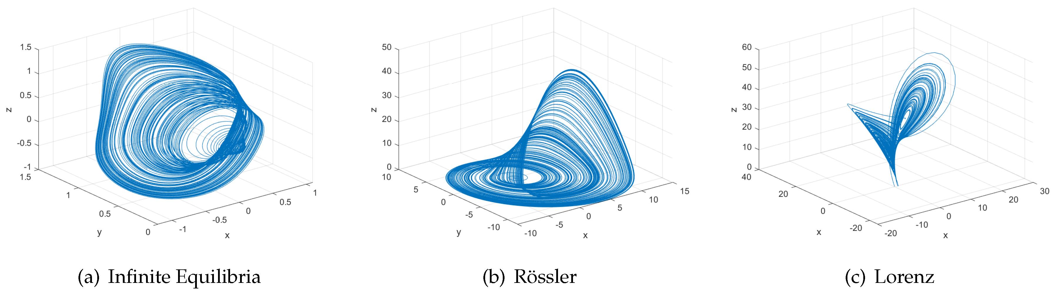
2. Chaotic Systems
3. Differential Evolution and Particle Swarm Optimization Algorithms
3.1. Differential Evolution Algorithm
| Algorithm 1 Differential Evolution |
Require:D, G, , , F, and .
|
3.2. Particle Swarm Optimization Algorithm
| Algorithm 2 Particle Swarm Optimization |
Require:D, G, , , , and .
|
4. Maximizing D
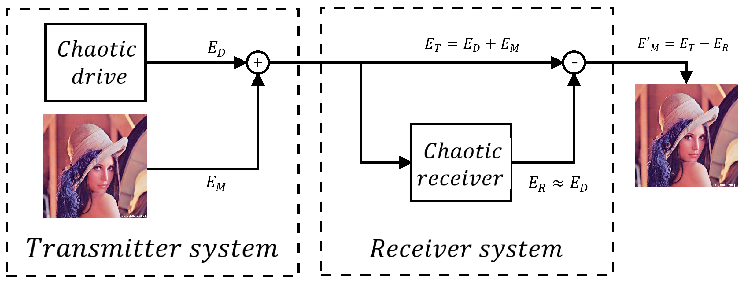
5. Encrypting Color Images Using State Variables with High D and LE+
6. Conclusions
Author Contributions
Funding
Conflicts of Interest
References
- Wolf, A.; Swift, J.B.; Swinney, H.L.; Vastano, J.A. Determining Lyapunov exponents from a time series. Phys. D Nonlinear Phenom. 1985, 16, 285–317. [Google Scholar] [CrossRef]
- Chen, H.; Bayani, A.; Akgul, A.; Jafari, M.A.; Pham, V.T.; Wang, X.; Jafari, S. A flexible chaotic system with adjustable amplitude, largest Lyapunov exponent, and local Kaplan–Yorke dimension and its usage in engineering applications. Nonlinear Dyn. 2018, 92, 1791–1800. [Google Scholar] [CrossRef]
- Petrzela, J.; Polak, L. Minimal Realizations of Autonomous Chaotic Oscillators Based on Trans-Immittance Filters. IEEE Access 2019, 7, 17561–17577. [Google Scholar] [CrossRef]
- Vaidyanathan, S.; Abba, O.A.; Betchewe, G.; Alidou, M. A new three-dimensional chaotic system: Its adaptive control and circuit design. Int. J. Autom. Control 2019, 13, 101–121. [Google Scholar] [CrossRef]
- Khan, A.; Kumar, S. Analysis and time-delay synchronisation of chaotic satellite systems. Pramana 2018, 91, 49. [Google Scholar] [CrossRef]
- Saad, A.B.; Boubaker, O. Bifurcations, chaos and synchronization of a predator–prey system with Allee effect and seasonally forcing in prey’s growth rate. Eur. Phys. J. Spec. Top. 2018, 227, 971–981. [Google Scholar] [CrossRef]
- Tlelo-Cuautle, E.; de la Fraga, L.G.; Pham, V.T.; Volos, C.; Jafari, S.; Quintas-Valles, A.D.J. Dynamics, FPGA realization and application of a chaotic system with an infinite number of equilibrium points. Nonlinear Dyn. 2017, 89, 1129–1139. [Google Scholar] [CrossRef]
- Rössler, O. An equation for continuous chaos. Phys. Lett. A 1976, 57, 397–398. [Google Scholar] [CrossRef]
- Lorenz, E.N. Deterministic nonperiodic flow. J. Atmos. Sci. 1963, 20, 130–141. [Google Scholar] [CrossRef]
- Petržela, J. Optimal Piecewise-Linear Approximation of the Quadratic Chaotic Dynamics. Radioengineering 2012, 21, 20–28. [Google Scholar]
- Li, S.Y.; Huang, S.C.; Yang, C.H.; Ge, Z.M. Generating tri-chaos attractors with three positive Lyapunov exponents in new four order system via linear coupling. Nonlinear Dyn. 2012, 69, 805–816. [Google Scholar] [CrossRef]
- Sun, Y.; Wu, C.Q. A radial-basis-function network-based method of estimating Lyapunov exponents from a scalar time series for analyzing nonlinear systems stability. Nonlinear Dyn. 2012, 70, 1689–1708. [Google Scholar] [CrossRef]
- Li, C.; Sprott, J.C. Amplitude control approach for chaotic signals. Nonlinear Dyn. 2013, 73, 1335–1341. [Google Scholar] [CrossRef]
- Storn, R.; Price, K. Differential Evolution—A Simple and Efficient Heuristic for global Optimization over Continuous Spaces. J. Glob. Optim. 1997, 11, 341–359. [Google Scholar] [CrossRef]
- Kennedy, J.; Eberhart, R. Particle swarm optimization. In Proceedings of the IEEE International Conference on Neural Networks, Perth, Australia, 27 November–1 December 1995; Volume 1000. [Google Scholar]
- Yang, C.; Zhu, W.; Ren, G. Approximate and efficient calculation of dominant Lyapunov exponents of high-dimensional nonlinear dynamic systems. Commun. Nonlinear Sci. Numer. Simul. 2013, 18, 3271–3277. [Google Scholar] [CrossRef]
- Dieci, L. Jacobian free computation of Lyapunov exponents. J. Dyn. Differ. Equ. 2002, 14, 697–717. [Google Scholar] [CrossRef]
- Rugonyi, S.; Bathe, K.J. An evaluation of the Lyapunov characteristic exponent of chaotic continuous systems. Int. J. Numer. Methods Eng. 2003, 56, 145–163. [Google Scholar] [CrossRef]
- Cardano, G.; Witmer, T. Ars Magna or the Rules of Algebra; Dover Books on Advanced Mathematics; Dover: Mineola, NY, USA, 1968. [Google Scholar]
- Guillén-Fernández, O.; Meléndez-Cano, A.; Tlelo-Cuautle, E.; Núñez-Pérez, J.C.; de Jesus Rangel-Magdaleno, J. On the synchronization techniques of chaotic oscillators and their FPGA-based implementation for secure image transmission. PLoS ONE 2019, 14, e0209618. [Google Scholar] [CrossRef] [PubMed]


| System | Parameters | LE | D |
|---|---|---|---|
| Infinite equilibria [7] | ∼0.17 | 2.0791 | |
| Rössler [8] | ; ; | 0.1300 | 2.0100 |
| Lorenz [9] | ; ; ; | 2.1600 | 2.0700 |
| System | Jacobian | Equilibrium Points |
|---|---|---|
| Infinite Equilibria | ||
| Rössler | ||
| Lorenz |  |
| Oscillator | Runs | DE | PSO | ||||
|---|---|---|---|---|---|---|---|
| Max D | Mean | Max D | Mean | ||||
| Infinite Equilibria | 1 | 2.0781 | 2.0789 | 0.02080 | 2.0764 | 2.0753 | 0.02059 |
| 2 | 2.0791 | 2.0788 | 0.02079 | 2.0767 | 2.0753 | 0.02036 | |
| 3 | 2.0781 | 2.0787 | 0.02071 | 2.0767 | 2.0759 | 0.02036 | |
| 4 | 2.0788 | 2.0787 | 0.02075 | 2.0716 | 2.0765 | 0.02073 | |
| 5 | 2.0785 | 2.0787 | 0.02063 | 2.0740 | 2.0738 | 0.02077 | |
| 6 | 2.0786 | 2.0785 | 0.02026 | 2.0766 | 2.0715 | 0.02039 | |
| 7 | 2.0781 | 2.0788 | 0.02043 | 2.0766 | 2.0734 | 0.02077 | |
| 8 | 2.0782 | 2.0788 | 0.02031 | 2.0754 | 2.0751 | 0.02031 | |
| 9 | 2.0786 | 2.0789 | 0.02051 | 2.0754 | 2.0752 | 0.02054 | |
| 10 | 2.0789 | 2.0787 | 0.02070 | 2.0737 | 2.0736 | 0.02045 | |
| Rössler | 1 | 2.0250 | 2.0395 | 0.02036 | 2.0235 | 2.0230 | 0.03285 |
| 2 | 2.0350 | 2.0377 | 0.02043 | 2.0225 | 2.0224 | 0.03286 | |
| 3 | 2.0510 | 2.0364 | 0.02046 | 2.0270 | 2.0210 | 0.03286 | |
| 4 | 2.0300 | 2.0374 | 0.02048 | 2.0229 | 2.0240 | 0.03289 | |
| 5 | 2.0500 | 2.0381 | 0.02038 | 2.0198 | 2.0220 | 0.03285 | |
| 6 | 2.0203 | 2.0383 | 0.02039 | 2.0269 | 2.0240 | 0.03288 | |
| 7 | 2.0203 | 2.0363 | 0.02028 | 2.0233 | 2.0230 | 0.03288 | |
| 8 | 2.0204 | 2.0373 | 0.02044 | 2.0170 | 2.0240 | 0.03287 | |
| 9 | 2.0204 | 2.0405 | 0.02026 | 2.0254 | 2.0230 | 0.03285 | |
| 10 | 2.0055 | 2.0414 | 0.02039 | 2.0265 | 2.0220 | 0.03287 | |
| Lorenz | 1 | 2.0754 | 2.0773 | 0.01486 | 2.0719 | 2.0713 | 0.00969 |
| 2 | 2.0730 | 2.0732 | 0.01481 | 2.0718 | 2.0712 | 0.00969 | |
| 3 | 2.0843 | 2.0783 | 0.01466 | 2.0706 | 2.0703 | 0.00969 | |
| 4 | 2.0791 | 2.0775 | 0.01478 | 2.0712 | 2.0705 | 0.00969 | |
| 5 | 2.0785 | 2.0772 | 0.01474 | 2.0712 | 2.0702 | 0.00969 | |
| 6 | 2.0839 | 2.0770 | 0.01486 | 2.0662 | 2.0710 | 0.00969 | |
| 7 | 2.0796 | 2.0752 | 0.01487 | 2.0690 | 2.0702 | 0.00969 | |
| 8 | 2.0739 | 2.0738 | 0.01479 | 2.0684 | 2.0708 | 0.00969 | |
| 9 | 2.0733 | 2.0733 | 0.01451 | 2.0692 | 2.0703 | 0.00969 | |
| 10 | 2.0741 | 2.0740 | 0.01431 | 2.0714 | 2.0744 | 0.00969 | |
| Oscillator | DE | PSO | ||||
|---|---|---|---|---|---|---|
| Design Parameters | LE | D | Design Parameters | LE | D | |
| Infinite Equilibria | a = 0.1006 | 0.0753 | 2.0791 | a = 0.0937 | 0.0753 | 2.079 |
| a = 0.0938 | 0.0730 | 2.0789 | a = 0.1007 | 0.0788 | 2.0789 | |
| a = 0.0939 | 0.0726 | 2.0786 | a = 0.1028 | 0.0796 | 2.0796 | |
| a = 0.0935 | 0.0726 | 2.0785 | a = 0.0935 | 0.0726 | 2.0785 | |
| a = 0.1007 | 0.0747 | 2.0788 | a = 0.1007 | 0.0787 | 2.0791 | |
| Rössler | a = 0.3609 b = 0.1000 c = 11.3470 | 0.2711 | 2.07890 | a = 0.3609 b = 0.1000 c = 11.3470 | 0.2711 | 2.02700 |
| a = 0.3947 b = 0.5490 c = 9.12060 | 0.2600 | 2.07140 | a = 0.3947 b = 0.5490 c = 9.12060 | 0.2600 | 2.02690 | |
| a = 0.3720 b = 0.2055 c = 12.0147 | 0.2710 | 2.07870 | a = 0.3947 b = 0.2055 c = 9.12060 | 0.2600 | 2.02650 | |
| a = 0.3930 b = 0.8505 c = 13.0501 | 0.2645 | 2.07810 | a = 0.3930 b = 0.8505 c = 13.0501 | 0.2645 | 2.02350 | |
| a = 0.3643 b = 0.1537 c = 12.7643 | 0.2764 | 2.07880 | a = 0.3643 b = 0.1537 c = 12.7643 | 0.2764 | 2.02330 | |
| Lorenz | 3.3129 | 2.08430 | 3.3129 | 2.07230 | ||
| 3.3122 | 2.08390 | 3.3122 | 2.07290 | |||
| 3.3168 | 2.07960 | 3.3168 | 2.07190 | |||
| 3.3149 | 2.07910 | 3.3149 | 2.07197 | |||
| 3.3199 | 2.07410 | 3.3199 | 2.07179 | |||
| Oscillator | D | State Variables | Correlation |
|---|---|---|---|
| Infinite Equilibria | 2.0791 | x | 0.0332 |
| y | 0.0589 | ||
| z | 0.0371 | ||
| 2.0789 | x | 0.0447 | |
| y | 0.2961 | ||
| z | 0.0423 | ||
| Rössler | 2.0789 | x | 0.1144 |
| y | 0.0075 | ||
| z | 0.0112 | ||
| 2.0788 | x | 0.0084 | |
| y | 0.0038 | ||
| z | 0.0034 | ||
| Lorenz | 2.0843 | x | 0.0173 |
| y | 0.0152 | ||
| z | 0.0025 | ||
| 2.0839 | x | 0.0009688 | |
| y | 0.0029 | ||
| z | 0.0010 |
© 2019 by the authors. Licensee MDPI, Basel, Switzerland. This article is an open access article distributed under the terms and conditions of the Creative Commons Attribution (CC BY) license (http://creativecommons.org/licenses/by/4.0/).
Share and Cite
Silva-Juarez, A.; Rodriguez-Gomez, G.; de la Fraga, L.G.; Guillen-Fernandez, O.; Tlelo-Cuautle, E. Optimizing the Kaplan–Yorke Dimension of Chaotic Oscillators Applying DE and PSO. Technologies 2019, 7, 38. https://doi.org/10.3390/technologies7020038
Silva-Juarez A, Rodriguez-Gomez G, de la Fraga LG, Guillen-Fernandez O, Tlelo-Cuautle E. Optimizing the Kaplan–Yorke Dimension of Chaotic Oscillators Applying DE and PSO. Technologies. 2019; 7(2):38. https://doi.org/10.3390/technologies7020038
Chicago/Turabian StyleSilva-Juarez, Alejandro, Gustavo Rodriguez-Gomez, Luis Gerardo de la Fraga, Omar Guillen-Fernandez, and Esteban Tlelo-Cuautle. 2019. "Optimizing the Kaplan–Yorke Dimension of Chaotic Oscillators Applying DE and PSO" Technologies 7, no. 2: 38. https://doi.org/10.3390/technologies7020038
APA StyleSilva-Juarez, A., Rodriguez-Gomez, G., de la Fraga, L. G., Guillen-Fernandez, O., & Tlelo-Cuautle, E. (2019). Optimizing the Kaplan–Yorke Dimension of Chaotic Oscillators Applying DE and PSO. Technologies, 7(2), 38. https://doi.org/10.3390/technologies7020038