1. Introduction
Cyber-physical systems (CPS) couple embedded processing tightly with its environment by incorporating I/O, sensors, and actuators to support interaction between smart objects and users. They enable context-aware services and applications that have become a desired feature in smart homes, smart industries, and advanced e-health solutions.
One of the research topics that has recently gained increasing attention is the automatic detection of a user’s currently performed activities, called online activity recognition. While machine learning has become a dominant approach, the classification of activities with statistical, signal-based, and frequency-domain-specific features, calculated from body-worn sensor signals, still allows for desirable fine-tuning towards resource-efficient configurations by domain knowledge. To enable unobtrusive systems, the use of wireless, body-worn sensors is unavoidable. However, like all other classes of CPS, their energy-efficient design is still of major concern, as it directly influences the battery lifetime and thus the usability of the system. General statements about the energy efficiency of such systems are difficult to make, as sensor modalities, feature sets, and classifiers vary among different classification goals. In order to address these difficulties, methods to estimate the energy consumption of a particular activity recognition configuration are necessary at design time.
In this article, a method to estimate the energy consumption of wireless sensor nodes for application-specific configurations is introduced. The estimation is based on dataflow models and analysis techniques, which have already become a de facto standard for signal processing, streaming, and multimedia applications. Based on these methods, we propose a novel approach for the estimation of energy consumption of wireless sensor nodes within the context of online activity recognition. In our experiments, we verified that our methods offer enough accuracy to substantiate early design decisions at the system level by comparing their results to energy consumption measurements of various widely used activity recognition configurations. The contribution of this article is thus twofold: (1) a formal modeling approach for activity recognition systems is introduced and (2) dataflow-based analysis techniques are extended to support energy estimation in early design stages.
The remainder of the article is structured as follows. In
Section 2, related work is discussed, which is followed by an introduction to the target application domain in
Section 3. The formal modeling techniques on which the presented concept is based is introduced in
Section 4. This is followed by
Section 5, which describes how activity recognition software can be modeled at different levels of abstraction by the proposed formalisms. The extension of the model-based analysis techniques to enable energy estimations at design time are explained in
Section 6. The experiments to evaluate the proposed concept are presented in
Section 7.
2. Related Work
Many works exist that have studied the model-based design of streaming applications with dataflow graphs. Important properties of the modeled application that can be analyzed from its graph representations involve throughput [
1], throughput-buffering trade-offs [
2], average and worst-case performance [
3,
4], latency and response time [
5,
6], and many others. In [
7], dataflow graphs were used for modeling and analyzing the performance of online gesture recognition.
Related to energy efficiency, there exist works that reduced the energy consumption of processor cores through dynamic voltage and frequency scaling (DVFS) while guaranteeing certain throughput constraints by using dataflow-based analysis techniques. Furthermore, in [
8], energy-aware task-mapping and scheduling optimization techniques for heterogeneous multi-processor system on chips (MPSoC) was studied. Instead of multi-objective optimization, our article is concerned with the modeling of activity recognition systems and their mapping to the distributed hardware platform of wireless sensor nodes and their data-aggregating hubs, such as smartphones. Furthermore, an energy consumption estimation approach for application-specific configurations of the activity recognition systems is shown.
Several works in the literature have studied the energy-efficient design of online activity recognition with wearable devices. Some of the approaches include disabling hardware sensors using prediction of activities [
9,
10], feature selection strategies to reduce the computational load [
11], classifier selection [
12], or fixed-point arithmetic [
13]. Other approaches, orthogonal to those aforementioned, study the on-board calculation of the feature extraction stage of activity recognition systems. In [
14,
15,
16,
17,
18,
19], it was shown that calculating features on the wireless sensor nodes could reduce the energy consumption of their wireless transceivers or flash memories due to the reduced amounts of data.
While [
20] already indicated a need for a trade-off between communication reduction and added computational effort, we have shown in [
21] how a trade-off for an application-specific configuration can be estimated at design time. This was done by using energy models of the hardware components.
In this article, we combine the recent findings of energy consumption estimation and state-of-the-art formal model-based design and analysis methods. Our contributions are a model-based design methodology for energy-efficient wireless sensor nodes in the context of online activity recognition and an approach for estimating energy consumption from dataflow models in early design stages.
3. Application Domain
In many approaches to online activity recognition, multiple sensors are attached to the human body which collect multidimensional signals from different sensor modalities, such as accelerometers, gyroscopes, magnetometers, and many others. From these signals, activity recognition software attempts to detect the currently performed activity of the human.
Since the first attempts towards recognizing activities with wearable sensors, a common processing chain very similar to a general pattern recognition pipeline has been established. This workflow, referred to as the activity recognition chain (ARC) [
22], is shown in
Figure 1 and contains five processing stages: data acquisition, preprocessing, segmentation, feature extraction, and, finally, classification.
While there are some approaches using adaptive segmenting of the sensor data stream, sliding window methods, most commonly with partial overlapping, is still the prevalent method of the segmentation stage [
23,
24,
25,
26,
27]. Based on these segments, a set of descriptive features for the anticipated activities is calculated at the feature extraction stage. Time-domain features are used very often, as they require low processing and usually show a high performance in terms of latency and throughput. The most common are mean, variance, skewness, kurtosis, zero/threshold crossing rate, or frequency-domain features like energy, frequency bands, etc. [
28,
29,
30]. Since this stage often drastically reduces the data rate, as a relatively small number of features is calculated from a large number of samples of a window, it was subject to a lot of research to perform this stage as near to the sensor as possible, i.e., on board of a wireless sensor node [
14,
15,
16,
18,
19], or even on-sensor [
17,
21]. However, each application-specific setup varies in sensor sampling frequency, sliding window size, sliding window overlap, and number of features and their computational effort in calculating them. Thus, the amount of reduced communications and added computational effort changes for each setup and has to be traded off for each particular configuration [
19,
21].
In order to substantiate early design decisions, methods are necessary to estimate the resulting energy consumption at design time at high abstraction levels. Since activity recognition systems include many dataflow-oriented algorithms with little control flow, we propose to use design techniques based on dataflow graphs. For this purpose, we combined dataflow graph analysis methods with energy models [
21] for energy estimation of wireless sensor nodes.
By considering modern sensors which already include microcontrollers performing sensor preprocessing like low- or high-pass filters, sensor fusion, or sensor correction algorithms, the preprocessing stage of most ARCs is usually already performed on the sensor itself. Moreover, for multi-sensor setups, the classification stage is usually performed on data-aggregating hubs, since the information of multiple sensors has to be processed together to perform activity classification. Although parts of the classification algorithms could also be considered for shifting their processing near to the data source, i.e., wireless sensor nodes, or the sensor device itself, we present our model-based design approach, with a focus on the segmentation and feature extraction stage of typical ARCs.
4. Synchronous Dataflow Graphs
The concept of the presented modeling approach is based on
synchronous dataflow (
SDF) graphs, as described by [
31].
Definition 1. SDF Graph
An SDF graph consists of a set of vertices V, a set of edges , token consumption rates , token production rates , and an initial token distribution .
Furthermore, in line with [
1,
2], we use timed SDF graphs, where an execution time
, also referred to as
delay, is associated with each actor
.
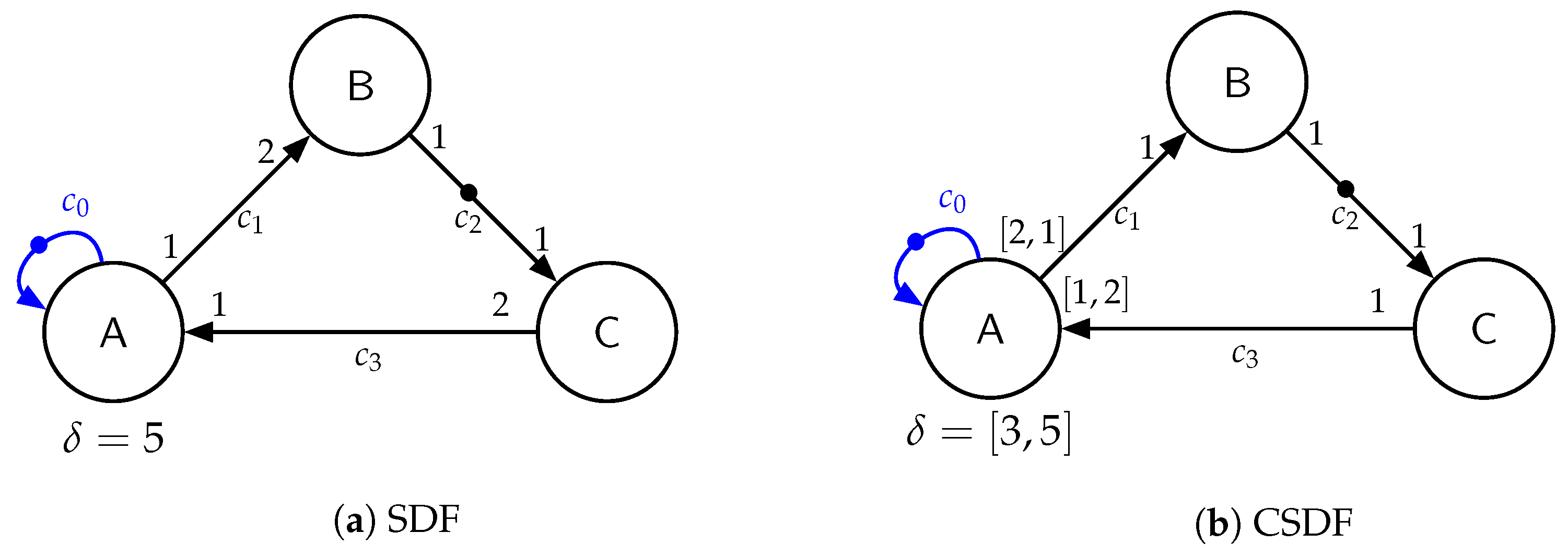
An example SDF graph can be seen in
Figure 2a. The vertices are called
actors (named A, B, and C in
Figure 2a) and represent function computations, which communicate data
tokens over unbounded
channels, with FIFO semantics represented by edges (
,
,
, and
in
Figure 2a). Hence, the presence and number of data packets are represented by tokens. With each channel, a number of
initial tokens is associated, marked with bullets in
Figure 2a on channel
and
. The consumption and production rates are annotated to the channel inputs and outputs and need to be fixed in SDF. Note that for the sake of simplicity, consumption and production rates not attached to the edges are assumed to equal 1, like channel
in
Figure 2a, and delays not attached are assumed to be
. The currently available number of tokens on a channel is denoted by
.
Definition 2. Actor Firing
An actor can be fired if the number of available tokens is greater or equal to the consumption rates of all its incoming channels , i.e., . If actor v fires, it consumes token from each incoming edge , and after its specified delay it produces token on each outgoing edge .
The execution of a consistent SDF graph forms fixed repetitive firing sequences caused by the constant production and consumption rates. Every such sequence is called an iteration and can be described by a repetition vector .
Definition 3. Repetition Vector
The repetition vector γ of an SDF graph G assigns a number of firings to each actor γ: . It is defined as the unique smallest non-trivial vector that satisfies the following balance equation: for each channel from actor to In this sense, non-trivial means that for all .
The repetition vector describes how often each actor fires during one iteration of the graph. Iff an SDF graph has a unique smallest non-trivial repetition vector, it is called consistent. This implies that the number of actor firings specified by the repetition vector has no net effect on the distribution of tokens on the channels, i.e., after a full iteration, the graph reaches a recurring state.
The execution of an SDF graph, where each actor fires as soon as its firing condition is met, is called a
self-timed execution [
2]. This furthermore allows multiple instances of an actor to fire simultaneously in parallel, allowing for maximum parallelization. This property is called
auto-concurrency. However, to limit or prevent auto-concurrency, self-edges to each actor can be added with as much initial tokens on it, as simultaneous firings of that actor are allowed. Thus, by adding only a single initial token on a self-edge, the corresponding actor can only fire in a non-overlapping fashion, and fires as soon as the delay of its previous firing has expired, at the earliest [
32]. This is shown in
Figure 2a for actor A in blue.
Another important property that can be calculated from an SDF graph is its throughput: [
1].
Definition 4. Throughput
The throughput is defined as the number of iterations of a time period divided by the duration of that period, i.e., the reciprocal of the average time duration of an iteration of the graph.
For a more detailed introduction to SDF graphs and their throughput analysis, we refer to [
1,
31].
The repetition vector of the example SDF graph in
Figure 2a is
and the execution time for one iteration is 10.
Cyclo-Static Dataflow
In [
33], the semantics of SDF was extended to
cyclo-static dataflow (
CSDF), with the concept of cyclic changing execution parameters of actors. In CSDF, following the more generalized definition from [
2], the delays
and production and consumption rates
and
do not necessarily need to be fixed anymore, but can change in fixed repetitive sequences, called
cycles. Furthermore, following the definition from [
2], the production rates
of channels connected to an actor
v, the consumption rates
of channels connected to an actor
v, and the delay
of actors
v are sequences having the same length
, i.e.,
. During the
ith firing, the actor
v consumes
tokens from each incoming channel
, produces
tokens on each outgoing edge
, and has a delay of
.
Note that, similar to SDF graphs, consumption and production rates not attached to the edges are assumed to equal 1 (e.g., channel
in
Figure 2b), delays not attached are assumed to be
, and single rates and delays of CSDF actors with multiple cycles are assumed to be equal in each cycle. The cyclic changing consumption and production rates, as well as the cyclic changing delays, can be seen on channel
,
, and actor A of the example CSDF graph in
Figure 2b, respectively. Its repetition vector is
. The execution time for one iteration is 8.
All the properties of SDF and CSDF graphs important for our modeling approach are implemented and publicly available as part of the SDF3 tools from [
34], which we used for analyzing the CSDF graphs in
Section 7.
5. Modeling of Activity Recognition
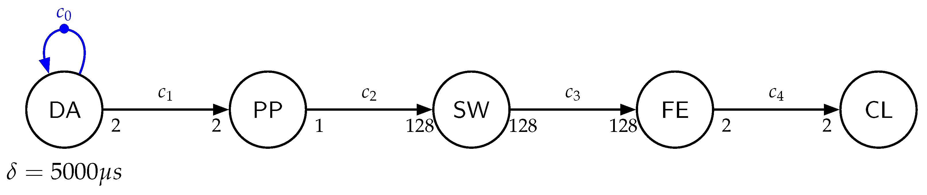
In this section, we show how online activity recognition systems can be modeled with (C)SDF semantics at different levels of abstraction. For this purpose, we modeled an ARC with example sampling periods, sensor modalities, sliding window parameters, and feature sets. Examining the activity recognition chain in
Figure 1, its different stages can be directly represented by SDF actors. In
Figure 3, an example SDF graph of an ARC is shown. The first actor, named DA, models the data acquisition stage as an example for an accelerometer and a gyroscope sampled at 200 Hz. The sampling frequency is modeled by a delay of
s and the self-edge
to prevent multiple simultaneous firings of the actor. The production rate on edge
is 2, modeling a 3D sample from each accelerometer and gyroscope. In the preprocessing (PP) stage, a sensor fusion takes both accelerometer and gyroscope samples and produces a single 3D orientation vector. This is modeled by the actor named PP, consuming two tokens from channel
and producing a single token on channel
each time PP fires. A sliding window of 128 samples is implemented at the segmentation stage, modeled by the actor named SW, consuming 128 tokens from channel
and producing 128 tokens on channel
at once. The actor named FE models the feature extraction stage. It consumes a full window of 128 tokens from channel
, calculates two features on its data, and produces the two features on channel
. Finally, the classification stage implements a classifier, which is modeled by the actor named CL, which consumes the two features from channel
and performs the classification. We omitted the output of this stage for the sake of simplicity. The repetition vector of the SDF graph shown in
Figure 3 is
.
For the sake of readability, actors SW and FE can be merged to actor FE, modeling the sliding window-based feature extraction. By doing so, their delays will be added, resulting in the same behavior of the graph.
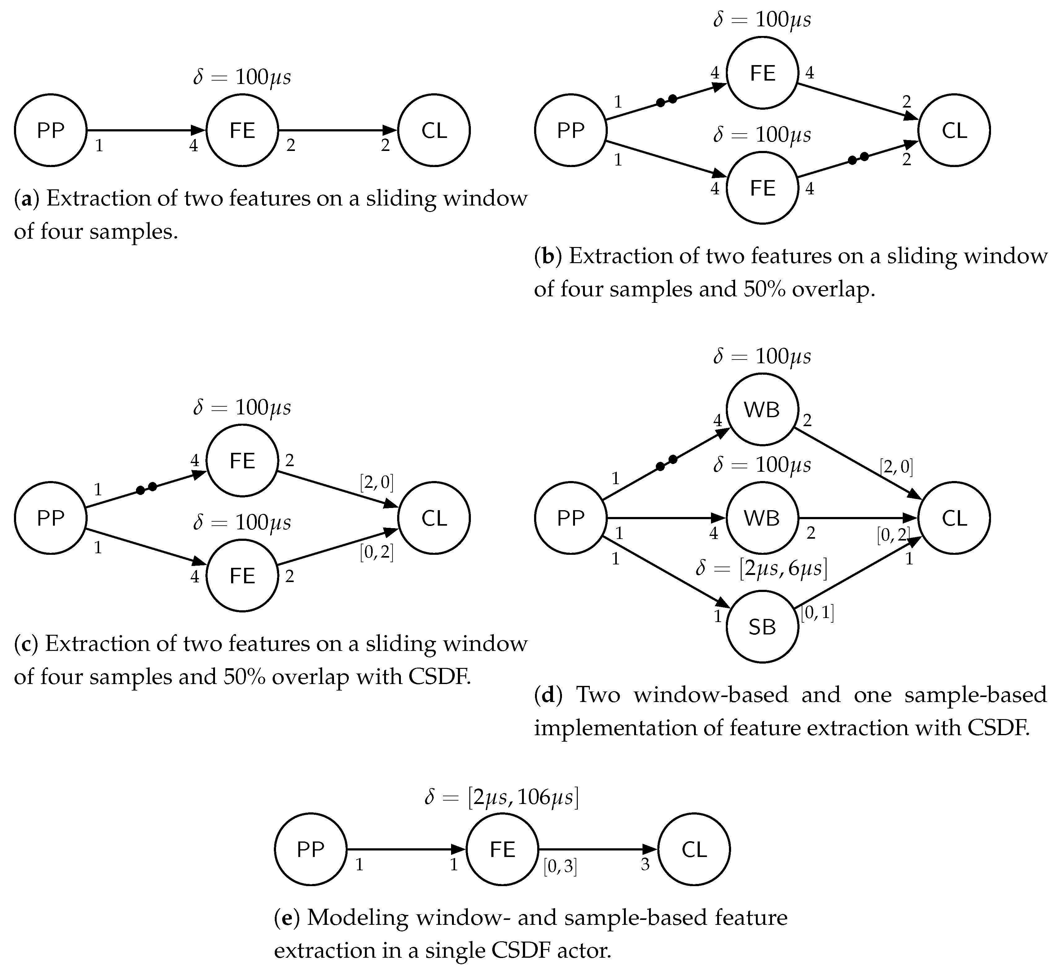
5.1. Detailed Application Modeling
An example of the resulting sliding window-based feature extraction is shown in
Figure 4a. Note that for the sake of readability the sliding window size
has been changed to 4 samples instead of 128. The actor FE is fired every four samples (after a new window is filled) and extracts two features that are produced on its outgoing edge. If a sliding window with an overlap is used, there are actually multiple sliding windows in parallel with a relative displacement defined by the overlap
. To model overlapping sliding windows, as many actors as parallel processed windows (
) are included, with an additional initial token to interleave the sliding windows with a displacement of
samples. See
Figure 4b for an example of the sliding window with
and
. However, modeling the overlapping sliding windows in SDF semantics requires also initial tokens on the output edges of the FE actors in order to synchronize the firing of the last actor CL. This results in a token production of the actors FE and a token consumption of actor CL that is actually higher than it would be implemented in software. To overcome this, CSDF semantics can be used to cycle the input rates of CL, matching the actual token consumption rate and reducing the token production rate of the actors FE to its real amount of calculated features. The principle is shown in
Figure 4c.
Up to now, we included the modeling of feature calculations on a whole window when it is filled, e.g., for a fast Fourier transform (FFT) calculation. However, some more time-efficient feature implementations update a value for the whole window but in a sample-based fashion, and finalize the value with the sample that fills the window. Examples are one-pass computations of statistical moments of arbitrary order [
35,
36], such as mean, variance, skewness, kurtosis, etc., which are often-used features in activity recognition [
23,
24,
28]. As an example, for computing the variance, with each new sample a sum is updated, and with the last sample belonging to that window the sum is updated and processed to calculate the actual variance from it for the whole window. In such sample-based feature extractions for whole windows, the actor should actually fire with each incoming sample but only produce an output, with the last sample finishing the window. This behavior can be captured with CSDF actors as well. If the updating of a sum takes
s for each new sample, and the finalizing for the last sample takes
s, the delay function of such an actor would be
and the corresponding production rate is
for a sliding window of
. Calculating two windows in parallel because of a window overlap of 50%, the actual delays and production sequences are superpositioned with a displacement of two samples, resulting in a periodical firing of two cycles with a delay of
and a production rate of
. This is included in
Figure 4d in actor SB together with the two window-based feature extractions WB, called FE previously.
To estimate energy consumption from the CSDF, it is necessary that the actual processing times of actors and the correct token consumption rates always match the implementation in order to extract the processor load and the transmission overhead on hardware communication channels, which we show in
Section 6. Furthermore, the unit of data, e.g., 3D floating point values, must kept constant when modeling it with tokens.
However, especially on wireless sensor nodes with integrated microcontrollers without task scheduling due to missing operating systems, feature extraction functions can be implemented in a sample-based fashion. This performs both the updating of the sample-based feature calculations with each new sample, and the buffering of samples for the last invocation for window-based processings, e.g., an FFT. These functions are invoked with each new sample and imply a static order scheduling of the different feature calculations inherently. Such implementation can be merged into a single actor summarizing the feature extraction calculations, which is shown in
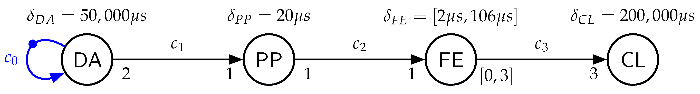
Figure 4e. The delay of actor FE summarizes the added processing times of all firing actors in each cycle, and their token production rate as well. This, on the one hand, simplifies the CSDF graph, but prevents the mapping of different feature calculations to different processing units and implies a certain scheduling of the actors. However, for the sake of simplicity, we continue with this level of abstraction in the following sections, without losing generality.
The full CSDF graph of the aforementioned example feature extraction, together with example delays for actor PP and actor CL, is shown in
Figure 5.
5.2. Hardware Model
The next step in designing the activity recognition system is to map the different software actors and communication channels to a hardware architecture. A
hardware model is a set of heterogeneous processing cores
P, a set of sensors
S, and set of directly connected wired or wireless communication channels
from the sensors
and to and between the processor cores
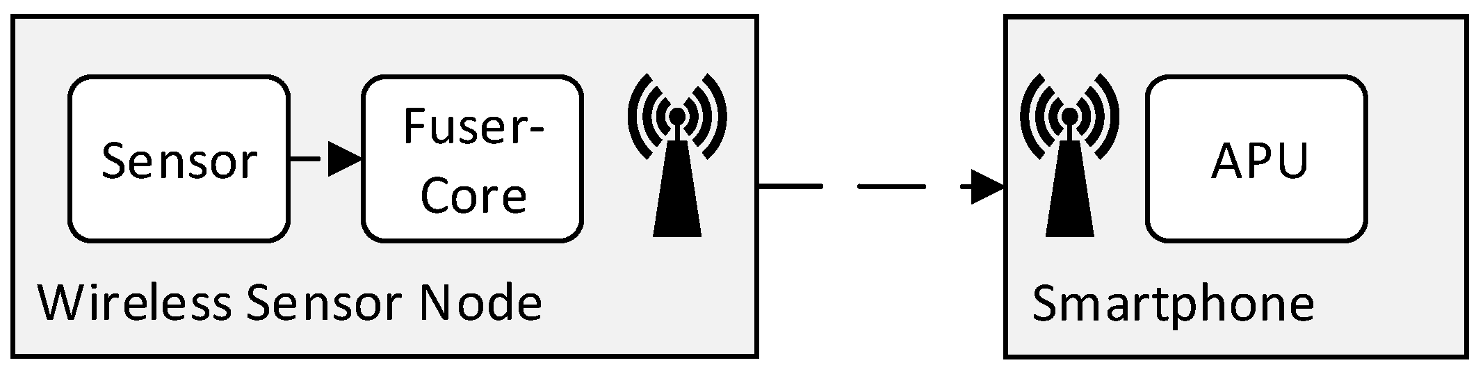
. An example platform for online activity recognition can be seen in
Figure 6, consisting of a wireless sensor board with an inertial sensor, an integrated microcontroller for sensor fusion (
FuserCore), and a wireless link, connecting the node with a smartphone with a more powerful application processing unit (APU). The corresponding hardware model consists of a sensor named SE, the FuserCore named FU, a hardware communication link (e.g., I
C) between them
, the smartphone processor named AP, and the wireless link (e.g., Bluetooth Low Energy) between them
. The hardware model can be seen in
Figure 7.
A mapping consists of a set of mapping relations between all actors V of a given dataflow graph G, and the union of processor cores P and sensors S of a hardware model H, with each actor mapped exactly once, i.e., with , and a set of mapping relations between all edges E of G and the hardware channels T of H, with each edge mapped exactly once, i.e., with . Furthermore, a mapping is only valid if the pair of actors connected by an edge are either mapped to the same processor/sensor or to processors/sensors which are directly connected by a hardware channel , i.e., , and the number of actors mapped to each sensor is maximal 1, i.e., .
After mapping the dataflow graph to the hardware, scheduling has to be found to serialize the executions of all actors mapped to the same processor in a non-overlapping way. There exist several works in the literature on the scheduling of SDF, CSDF, and dataflow graphs in general [
32,
37,
38,
39,
40,
41]. For our approach, scheduling needs to be integrated into the dataflow graph itself by adding additional actors and edges, as in [
32,
37,
38,
41], to allow performance evaluation with dataflow graph analysis techniques afterwards. To prevent auto-concurrency, we first introduce self-edges (
) to each actor. Secondly, a scheduling scheme has to be selected for different actors mapped to the same processor core. For our model in
Figure 7, a simple self-timed schedule is enabled by adding a feedback edge
from actor FE to PP. This prevents simultaneous firings of FE and PP. For detailed introductions on scheduling dataflow graphs we refer to the aforementioned literature. Note that the actors and edges added to
G for scheduling purposes are not contained in the mapping
M of graph
G.
6. Energy Consumption Estimation
To estimate energy consumption of a CSDF graph
G, a given mapping
M, and integrated scheduling, we first need to assign energy models to the hardware components we are interested in. We will use the example graph in
Figure 7. The most decisive hardware components whose energy consumption changes for different ARC setups are the sensor SE, the integrated FuserCore FU, and the wireless Bluetooth Low Energy (BTLE) link
. The energy consumption of the sensor will change among different sampling rates and sensor modalities, like the accelerometer and gyroscope [
42]. The energy consumption of the integrated processing core on the wireless sensor node is dependent on the computational load introduced by the on-board feature extraction, while the energy consumption of the wireless transmissions depend on the transmission rate between the wireless sensor node and the smartphone.
For each energy dependency case of a hardware component, we need to integrate a measure in the dataflow analysis which allows us to estimate the energy consumption of the wireless node. Similar to the penalty functions in weakly consistent scenario-aware dataflow graphs in [
43], we define an effort function for each component that we are interested in.
As the energy consumption of the sensor depends on its sampling frequency, the effort function
of a particular sensor
counts the number of firings during one iteration of the graph of that actor, which is mapped to hardware component
, i.e.,
, divided by the average iteration duration or multiplied by the throughput of the graph, respectively. The number of firings within one iteration can be acquired by calculating the repetition vector of the graph and using the corresponding entry
. The effort function
for the example graph in
Figure 7 is calculated by
.
For a particular processing core , the effort function captures its computational load. The load is defined as the accumulated time the core is actively processing within an observation period, divided by the duration of the period. It is intuitive to define the observation period as one graph iteration. The active processing time within one iteration can be calculated by summing up all delays of the actor firings mapped and scheduled on the processor of interest. This sum is then divided by the iteration period or multiplied by the throughput of the graph, respectively. Note that this is possible due to the integrated scheduling, as it prevent the simultaneous firings of actors mapped to the same processor. Thus, simply adding up all the delays of all occurring actor firings within one iteration on a processor core is sufficient to acquire the active time of the processor. The pseudo-code in Algorithm 1 shows how to calculate the effort function of the load of a particular processor core .
| Algorithm 1 Calculating effort function capturing the load of a processor core. p. |
- 1:
procedurecalculate_load_effort(p,G,H, M,, ) - 2:
- 3:
- 4:
for all in do - 5:
- 6:
for all j in do - 7:
- 8:
end - 9:
end - 10:
return
|
The algorithm gets the target processor p as its first parameter, together with the CSDF graph G, the hardware model H, a mapping M, the repetition vector of G, and the throughput of G. The function returns the set of actors that are mapped to the processor core p. In line 4, it is iterated over this set, saving the repetition vector entry of each actor to variable n in line 5. In line 7, the delays of all cycles within the n firings of actor are summed up in variable . This is repeated for all actors by the loop in line 4. At the end in line 10, is multiplied with the throughput of graph G and returned.
To acquire the effort function accounting for the transmission rate over the wireless BTLE link, we need to identify all channels mapped to it, and count the number of token productions from all actors producing tokens on those channels during one graph iteration. This can be done by iterating through all cycles of each actor connected to those channels as source actors, and accumulating all the production rates within one graph iteration. The repetition vector entries of those actors define how often we have to iterate through the cycles. The accumulated number of produced tokens is then divided by the iteration period of the graph or multiplied by its throughput, respectively. The principle is shown in Algorithm 2.
| Algorithm 2 Calculating effort function , capturing the amount of transmission on hardware channel t. |
- 1:
procedurecalculate_transmission_effort(t,G,H, M,, ) - 2:
- 3:
- 4:
for all in do - 5:
- 6:
- 7:
for all j in do - 8:
- 9:
end - 10:
end - 11:
return
|
The algorithm gets the target hardware channel t as its first parameter, together with the CSDF graph G, the hardware model H, a mapping M, the repetition vector of G, and the throughput of G. The function returns the set of channels that are mapped to the hardware channel t. Over this set it is iterated in line 4. In each iteration, the source actor of channel is returned by function in line 5, and its repetition vector entry is saved to variable n in line 5. In line 7, over all cycles actor ’s n firings are iterated, its production rates to channel are summed in variable in line 8. This is repeated for all channels in by the loop in line 4. At the end in line 11, will be multiplied with the throughput of graph G and returned.
Note that for acquiring the effort functions, only actors and channels of the original dataflow graph are taken into account, excluding additional actors and channels introduced for mapping and scheduling.
Energy Models of Hardware Components
The major components in the presented energy estimation approach are energy models of the decisive parts of the target architecture, that model the energy consumption changes depending on a certain parameter. The sensor is the first component in the processing chain, whose power consumption depends on it’s sampling frequency. As an example, the ultra low-power sensor hub BHI160 [
42] has low power modes, in which duty cycles between the sampling times power down the sensing hardware to improve energy consumption. The data sheet provides the power consumption of sensor combinations at different sampling frequencies. This provides enough information for an energy estimation. The effort function
functions as the parameter for the energy model of the target sensor configuration. The power consumption of the sensor is given as a dependency on the sampling frequency, which is in line with the defined effort function
.
The energy consumption of the integrated FuserCore depends on its computational load. In [
21], we have shown that its energy consumption is linear to the processing load introduced to the integrated FuserCore, and how a simple energy model can be built from it if not available within the data sheet. The fitted energy model is accurate enough to estimate the energy consumption of different feature extraction configurations executed on it. The energy model takes the computational load, as defined in
Section 6, as a parameter and can take the effort function
directly as its input.
The component with the highest influence on the wireless sensor node’s energy consumption is the wireless link [
17]. In [
21], we have shown how to build a similar energy model of a BTLE transceiver which is directly dependent on the number of BTLE packets sent in a specified time interval, i.e., with a certain frequency. In general, such a model has to be converted into the appropriate data unit when using effort function
as its input parameter. The effort function
counts token productions on the hardware channel
per time unit, i.e., token production frequency. In our dataflow model, a token models a 3D floating point value, which in this case is in line with the energy model from [
21], as one BTLE packet contains one 3D floating value as well. However, for the general case, it needs to be mentioned that a conversion into the appropriate data unit might be necessary if the data unit of tokens does not match the energy model’s input parameter.
The differences of each effort function of two configurations are used to calculate the difference in energy consumption of each component of the two configurations by using their energy models. In order to estimate an absolute energy consumption of a configuration, a measurement of a reference configuration is needed. This can be any configuration which is easy to deploy without additional engineering overhead, which will be shown in
Section 7.
7. Experiments
For our experiments, we implemented the setup shown in
Figure 6 consisting of a Samsung Galaxy S5 smartphone and a custom wireless sensor node. The sensor node ships with a Bosch BHI160 Ultra-Low-Power Sensor Hub [
42] containing an accelerometer, an gyroscope, and an integrated 32-bit floating-point microcontroller, referred to as
FuserCore. Furthermore, a DIALOG DA14583 system-on-chip (SoC) with an integrated BTLE radio transceiver and baseband processor is used to acquire the sensor data from the BHI160 over I
C and send it via BTLE to the smartphone. The board is powered by a CR1225 coin cell battery at 3 V. The overall power consumption of sending raw accelerometer data at 100 Hz via BTLE is ≈ 4 mW. All implementations of on-board feature extraction were performed on the BHI160’s integrated FuserCore. The DIALOG controller is mainly used for packing end sending BTLE packets.
7.1. Energy Measurements
For measuring the energy consumption of the wireless sensor node, we used the approach from [
44], as it is easy to deploy and meets the necessary requirements to compare average energy consumption of different configurations. We used a
shunt resistor in series with a constant 3 V power supply and a DSO-X 3034A oscilloscope from Agilent Technologies to measure the average voltage drop over the shunt over a time of at least 100 s per measurement. Due to its proportional nature, the average energy consumption can be deduced from the measured average voltage drop with sufficient accuracy. The temperature dependency was considered to be neglectable in our setup, which could be substantiated with our acquired results. When comparing the average voltage drop of different configurations, the systematic error of the measuring apparatus and the tolerance of the shunt resistor are canceled out, and thus, propagation of uncertainty can be neglected for our evaluations. From all measurements of the voltage drop over the shunt, we calculated the power consumption presented in
Section 7.4.
7.2. Model Calibration
Since our custom sensor node is not shipped with any energy models for the FuserCore or the BTLE transceiver, we followed the same approach as we did in [
21] to acquire those models. We implemented nine calibration configurations, starting with a baseline of sending raw accelerometer data sampled at 100 Hz via Bluetooth. From this calibration configuration, we synthetically reduced the output data rate of the sensor by implementing four additional configurations in its firmware to only send every 2nd, 4th, 8th, or 16th sample, respectively. This only reduces the output data rate of the sensor, without changing its sampling frequency or power mode. The BTLE packets contained 3D floating point values. By calculating a linear regression over the five measurements, we acquired the dependency of its energy consumption from the output data rate by using the regression slope. We did this for five devices of the custom sensor node and used the mean slope of their regressions.
The same was done for acquiring the energy dependency of the FuserCore. Here we started again with the baseline calibration configuration of sending raw accelerometer data at 100 Hz and implementing four different firmware versions, each introducing artificial computational load, by calculating multiply and accumulate operations in a loop with different loop counters. We measured the computation time of executing the loop and, together with the sampling period of 10 ms with which this code is performed, we calculated the computational load introduced in each configuration. Together with the measured average voltage drops, we calculated a linear regression again over the five devices and used the mean regression slope as the energy model for the FuserCore.
The acquired energy dependency for the BTLE transceiver is 0.01191546 mW/Hz and the energy dependency of the FuserCore is 0.02138247 mW/workload %. The energy consumption for different sensor modalities and sampling frequencies were taken from the BHI160’s data sheet [
42]. The baseline calibration configuration that sends raw sensor data sampled at 100 Hz without additional processing on the FuserCore is also our reference configuration, from which we estimated all test configurations by our dataflow-based approach in the next section.
7.3. Dataflow Evaluation
We implemented six test configurations of on-board feature extractions or sending raw sensor data on the wireless sensor node with varying sampling frequencies, sliding window length, window overlaps, feature combinations, and mappings. The settings of each configuration and the reference configuration for the energy models can be seen in
Table 1. In column
Sensor, the sensor modality of each configuration is shown, which is either the accelerometer, the gyroscope, or both. The column
describes the sampling frequency of each sensor that is used. If both accelerometer and gyroscope is used, the sampling frequency applies to both. The next column specifies the size of the sliding window in
number of samples from each sensor modality. The column
Window Overlap gives the overlap of the sliding windows. Column
Features shows the implemented feature set on the sliding window calculated for each dimension of all used sensor modalities. The feature set
MVSKPE is composed of features which have shown good recognition performance in a kitchen task assessment scenario [
24]. The feature set is a combination of sample-based processing of Mean, Variance, Skewness, and Kurtosis, and a window-based processing of an FFT where the peak frequency and its magnitude (referred to as Energy in [
24]) are used as features. This sums up to six features calculated for each dimension of the sensor data. The feature set
MV is a set of sample-based processing of the two features Mean and Variance only. The feature ∫ is an integral over the raw data of each dimension of the sensor signal within the sliding window. The last column,
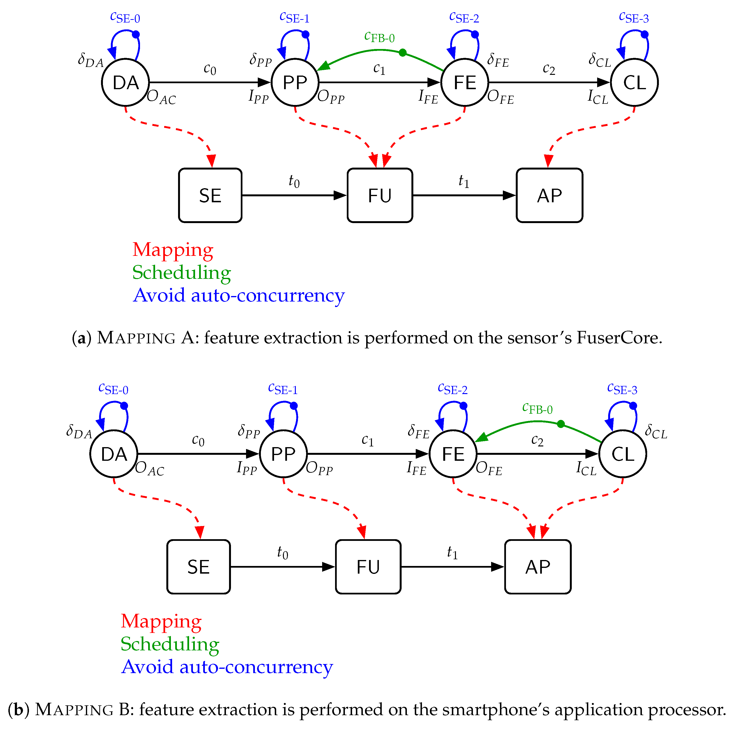
Mapping, specifies which mapping is used and refers to
Figure 8, showing
Mapping A and
Mapping B, i.e., calculating features on board of the wireless sensor node or sending raw data to the smartphone. Note that in configurations with
Mapping B, the columns
Window Length,
Window Overlap, and
Features contain
ANY, since in these configurations the feature extraction would be performed on the smartphone and its configuration does not influence the energy consumption of the wireless sensor node.
The configurations in
Table 1 were chosen to have in each column a variation of parameters that influence the energy consumption of the wireless sensor node. This way, we covered all parameters that can be changed in a particular feature extraction setup to evaluate our approach. In total, this covers three combinations of sensor modalities of accelerometer, gyroscope, or both; sensor sampling frequencies of 50 Hz, 100 Hz, and 200 Hz; sliding window lengths of 50 or 128 samples; overlaps of
,
, and
; three different features sets; and two possible mappings of the feature extraction stage.
Each of the configurations has been modeled as a CSDF graph.
Figure 8 shows the general graph structures with parameterized input/output rates, actor delays, and two different mappings, namely, calculating the features on the sensor (
Mapping A), or calculating features on the smartphones, i.e., sending raw sensor data from the wireless sensor node (
Mapping B).
The corresponding parameters of each configuration can be found in
Table 2. Note that the reference configurations and C6 are used together with
Mapping B, i.e., they are configurations where the wireless sensor node is sending raw samples to the smartphone. Thus, the length of the sliding window, its overlap, and the calculated features are not important for the energy consumption of the wireless sensor node. However, in our graphs we chose configuration C3 with
Mapping B as the reference scenario, and C4 with
Mapping B as C6 to show the impact of shifting the feature extraction of these configurations to the wireless sensor node. The delays
and
are set to zero in the constructed dataflow graphs, as the classification is not part of the evaluation and the preprocessing stage is not changed among different configurations.
7.4. Results
The throughputs and repetition vectors of the CSDF graphs have been calculated using the SDF3 tools from [
34]. The effort functions have been acquired following the principle from
Section 6. The throughput of each graph, its repetition vector, the corresponding effort functions, and the predicted energy consumption from these graphs are summarized in
Table 3.
The actual measured energy consumption of all configurations on all five devices and their mean are shown in
Table 4. The prediction errors, i.e., the differences in the predicted values of energy consumption by the model and the measured consumption scaled with the measured values of all five devices and their mean, are summarized in
Table 5. The highest prediction error of
was achieved for configuration C3. This is on the one hand caused by an outlier with Sensor 3, but also a slightly higher prediction error for this configuration compared to the others. In general, the predicted energy consumption with the model-based approach is close enough to the measured values to substantiate early design decisions. Shifting the feature extraction of the reference configuration towards the sensor (C3) instead of sending raw data (reference configuration), we can predict a consumption of 3.0842 mV instead of 4.0513 mV. The measured consumption is 3.3164 mV (3.192 mV excluding S3), which deviates by 7.5% (3.4% if S3 is excluded) from the predicted value. However, the energy saving from C1 to C3 is predicted to be 23.9% and measured as 18.1% (21.2% excluding S3), which is accurate enough to substantiate at design time the decision of shifting the feature extraction to the sensor to save energy. Similarly, shifting the feature extraction from C6 to the sensor (C4) instead of sending raw data, the model-based approach predicts an energy saving of 30.3%, while the measured energy saving is about 30.2%. Other design decisions, like using an additional sensor, can be evaluated similarly. From configuration C1 to C3, the gyroscope was excluded from the setup. The predicted energy consumption saving of this change is 48.7%. The measured difference is about 45.3% (47.4% if interpreting the value of S3 as an outlier).
8. Discussion
In the previous section, we showed that we can predict the energy consumption of a wireless sensor node in different configurations and mappings of an ARC with a considerable estimation accuracy. Considering a mean prediction error of all configurations of ( excluding the outlier of Sensor 3 in configuration C3), a design decision which causes a change of energy consumption of less than is close to the range of prediction error, which might on the other hand not need an accurate prediction, as the potential energy saving is marginal for such cases anyway.
Thus, we evaluate the model-based energy prediction approach as a useful methodology at design time to substantiate design decisions impacting the energy consumption of wireless sensor nodes when designing online activity recognition systems. In the following, we discuss the benefits and limitations of the proposed design method.
8.1. Benefits
The model-based approach allows the comparison of different configurations and mappings of an ARC. These differences can also include energy efficiency strategies, such as sensor selection and feature selection approaches, often found in the literature [
9,
10,
11,
45]. They can be separately modeled and compared to their non-optimized counterparts, showing their impact on the energy consumption. The major benefit of the model-based approach is the estimation at design time, which avoids the actual time-consuming and error-prone implementation of different configurations in attempts to find the most energy-efficient design, which is refined later on. As an additional step compared to an ad hoc implementation, our proposed approach requires a model calibration. This requires either proper analysis methods, a lot of experience of the system designer (manual calibration), or the partial implementation of sub-functionalities, perhaps available through previous product versions. Nevertheless, the calibration typically only results in additional effort if the final system implementation is obvious in early design steps. Considering today’s systems complexity, which is expected to further increase in the future, the spent effort for modeling and calibration will be much less compared to implementing and checking all possible configurations of the system.
8.2. Limitations
The proposed modeling approach with CSDF is limited to the cyclo-static behavior of activity recognition. As an example, a context-aware activity recognition system that changes its configuration (e.g., dynamic sensor selection [
9,
10] or dynamic feature selection [
11,
45]) based on the situation cannot be fully captured by CSDF. The data-dependent context changes would require dataflow variants allowing the modeling of dynamic, data-dependent behaviors. Possible dataflow variants could be scenario-aware dataflow (SADF) [
4] or enable-invoke dataflow (EIDF) [
46]. In contrast to these, our proposed CSDF-based method could only model each configuration present in a context-aware activity recognition system individually and analyze them separately.
9. Conclusions and Future Work
In the article at hand, a formal modeling approach for activity recognition systems is introduced, which is based on dataflow graphs. Furthermore, dataflow analysis techniques are extended to enable estimations of the energy consumption of wearable sensor nodes at early design stages of the corresponding activity recognition system. The proposed modeling approach is shown at different levels of abstraction by applying it to the segmentation and feature extraction stages of typical activity recognition systems. The accuracy of the proposed energy estimation technique is evaluated on a set of configurations, composed of different sensor sampling frequencies, sensor modalities, sliding window parameters like size and overlap, sample-based and window-based feature sets, and mappings of either calculating features on board of wireless sensor nodes, or sending raw data over wireless channels. All configurations have also been implemented in a setup consisting of a custom low-power wireless sensor node and a smartphone. In our experiments, the energy consumption of the wireless sensor node estimated by our model-based approach is compared to the measured energy consumption values. We achieved a system-level average accuracy above 97%, which is accurate enough to substantiate decisions about the configuration of activity recognition systems at early design stages.
In our future work, we want to extend the proposed approach to activity recognition systems with dynamic changes in configuration, such as for context-awareness. Therefore, dataflow variants allowing the modeling of dynamic behavior will be subject to our research in the future.


