Fuzzy Logic and Regression Approaches for Adaptive Sampling of Multimedia Traffic in Wireless Computer Networks ^†

Abstract

Organisations such as hospitals and the public are increasingly relying on large computer networks to access information and to communicate multimedia-type data. To assess the effectiveness of these networks, the traffic parameters need to be analysed. Due to the quantity of the data packets, examining each packet’s transmission parameters is not practical, especially in real time. Sampling techniques allow a subset of packets that accurately represents the original traffic to be examined and they are thus important in evaluating the performance of multimedia networks. In this study, an adaptive sampling technique based on regression and a fuzzy inference system was developed. The technique dynamically updates the number of packets sampled by responding to the traffic’s variations. Its performance was found to be superior to the conventional nonadaptive sampling methods.

1. Introduction

The growing availability of mobile wireless devices such as tablets, smartphones, and wearable monitoring sensors have resulted in innovative technologies dedicated for organisations and individuals. A sector that has particularly benefitted from these technologies is healthcare. Several technologies have been reported for improving information access, enhancing patients’ experience, managing resources, and increasing the standard of treatment in healthcare environments. These include electronic health (eHealth), mobile health (mHealth), authentication and tracking, remote monitoring, consultation and diagnosis services, and mobile tele-monitoring [1]. These technologies and associated services are becoming increasingly real time and require computer networks with improved performance [2]. The transmission of multimedia traffic associated with these services over wired and wireless computer networks creates demands on bandwidth and other resources [2,3]. Also, there is a growing interest in remotely monitoring patients in their home environment rather than in hospitals [4,5,6,7,8]. The benefits provided by this approach include improved patient experience and potential reduction in healthcare costs. As patients’ safety depends on the correct operation of the supporting networks, they need to be reliable and to have an appropriate performance [9]. Numerous issues such as uncontrolled increase of traffic with respect to network capacity can degrade the network’s performance [10]. Therefore, to effectively manage these networks and to provide desired services to their users, suitable tools to assess their performance are needed. Quality of Service (QoS) encapsulates a set of tools, protocols, and approaches that allow network performance to be evaluated and improved and thus it plays an important role in managing multimedia networks. QoS facilitates network operations such as traffic shaping and policing, prioritising time-sensitive applications, and guaranteeing agreed resources for certain applications. Therefore, QoS mechanisms enable network service providers to customise their resources to the users’ needs and users to be able to determine whether their provisions conform to what they requested.

An approach to evaluating network performance using QoS involves analysing network traffic information. Traffic analysis requires packet transmission information for individual flows and the overall network to be gathered and interpreted. However, analysing transmission information for every packet is impractical in real time due to high computational requirements. Therefore, a subset of packets needs to be selected such that the number of packets in the subset is significantly smaller than the total number of transmitted packets while retaining the original traffic’s attributes. This operation is called sampling and plays an important role in evaluating a multimedia network’s performance [11,12,13]. Sampling can be performed adaptively or in a nonadaptive manner. Nonadaptive sampling methods do not consider variations in traffic dynamics when measuring traffic information [14,15]. Examples of nonadaptive sampling methods are systematic, random, and stratified. In systematic sampling, a packet is selected at a predefined fixed time interval or based on a fixed packet count. In random sampling, packets are selected at a random time intervals or based on a random packet count number. Stratified sampling combines random and systematic sampling methods by defining a fixed interval and choosing a packet randomly within the interval. Figure 1 illustrates systematic, random, and stratified sampling methods.

Adaptive sampling can be more effective as it increases the number of selected packets when the traffic variations are higher and chooses fewer packets during periods of reduced traffic activity. In this study, a linguistic information processing method called fuzzy logic was used to implement adaptive sampling. Systems that require complex mathematical models for their representation may be more conveniently expressed in fuzzy logic terms [16]. Fuzzy logic can be implemented in different ways, one of which is the Fuzzy Inference System (FIS), shown in Figure 2.

A FIS has six parts, i.e., numeric inputs, fuzzification, knowledge base, inference engine, defuzzification, and numeric outputs. Its inputs are generally expressed numerically. These values are processed to determine the degrees to which they belong to a number of predefined membership functions called fuzzy sets. The membership functions define the degrees (or extents) to which an input belongs to the specified fuzzy sets. Degree of membership ($\mu$) varies continuously from 0 (not a member) to 1 (full member). This operation is called the fuzzification of numeric inputs. For example, a traffic delay value can be fuzzified by the fuzzy sets low_delay, average_delay, and high_delay, resulting in different degrees of membership. Therefore, a value does not have to exclusively belong to a single fuzzy set as is the case in the crisp sets [17]. The inference engine performs inferencing and compares the fuzzified variables with the traffic knowledge coded in the knowledge base to draw conclusions about the inputs. Typically the coding of the knowledge in the knowledge base is achieved by using a series of IF-THEN rules. The IF part of the rule is called the antecedent or premise and the THEN part is called the consequent or conclusion. An example of a rule is IF delay is very_high THEN QoS is poor. The outputs from the inference engine are defuzzified to produce numeric values by using a number of output membership functions.

FIS has been previously used for adaptive sampling of computer network traffic [18,19]. The main differences between this study and those reported in [18,19] are that in this study the traffic was modelled using linear regression prior to using the FIS and a physical rather than a simulated network was used.

Regression analysis is a technique for exploring the relationship between dependent and independent variables [20,21,22]. Regression can be linear or nonlinear, but linear regression is more commonly used for predictive and for analysis tasks and is the type used in this study. Regression models have been used for sensor networks, allowing their processes to be predicted based on the current captured data or based on the nearest network node [23]. This leads to a reduction in the amount of transmitted data packets.

In our study, the output from the regression model was interpreted using fuzzy logic. The main contribution of this study is the development of a novel adaptive sampling technique that can simultaneously sample three main traffic parameters—delay, jitter, and percentage packet loss ratio—in a physical computer network. The method can quantify the overall network QoS for multimedia networks.

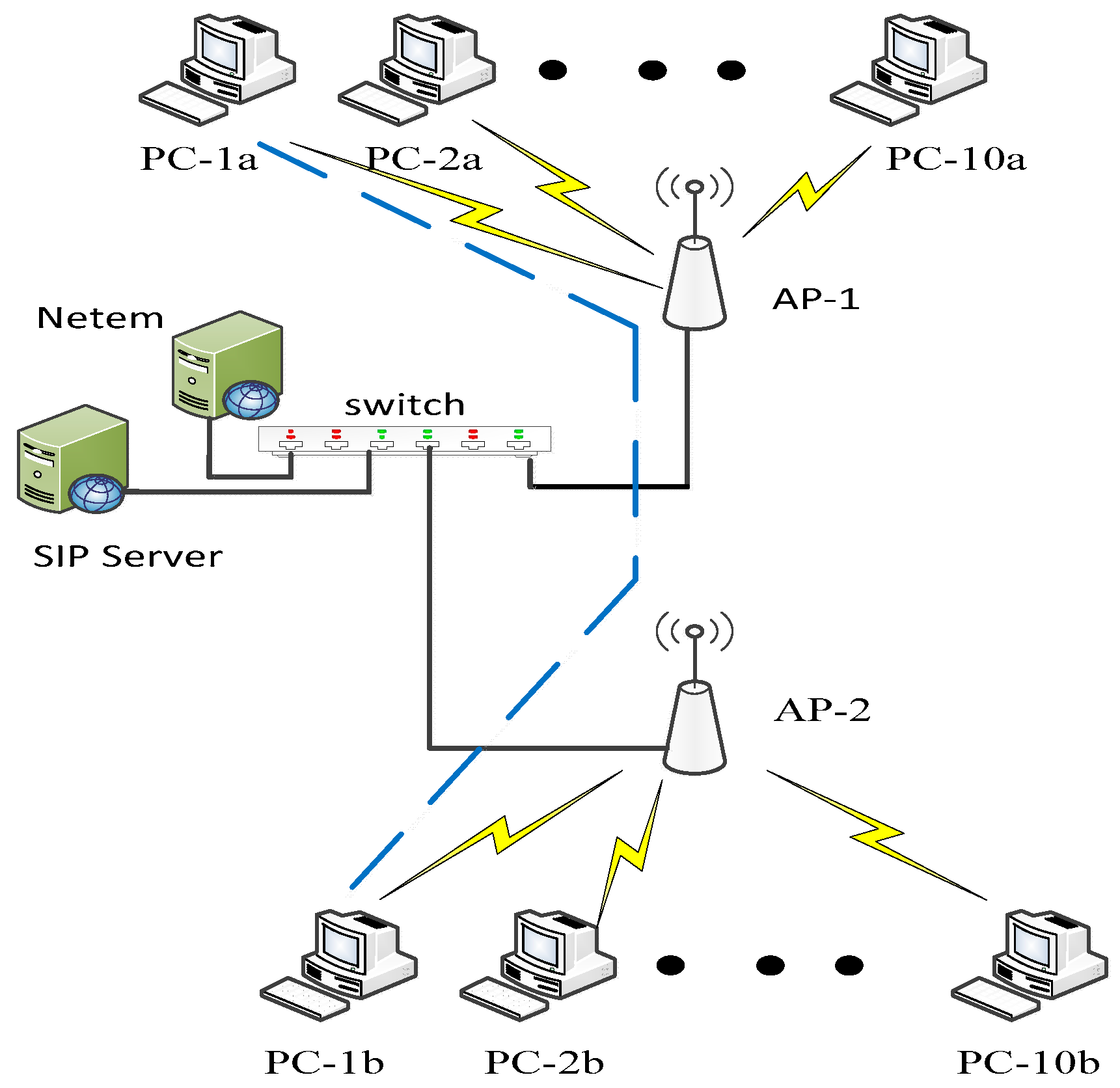
2. Materials and Methods

The developed adaptive sampling method was evaluated using a wireless computer network (shown in Figure 3) set up in a network research laboratory with an area of 4 m × 6 m. The aim was to explore how well the adaptively sampled traffic represents the original traffic for QoS assessment.

The network consisted of two Cisco^© AIR-AP1852E access points (APs) operating using the IEEE 802.11ac/n Wi-Fi protocol. Cisco^© APs contain four external dual-band antennas. A Cisco^© catalyst 3560-CX switch connected the two APs with a Session Initiation Protocol (SIP) server via 1 Giga bits per second (Gbps) wired links. The specifications of the personal computers (PCs) used in the study were as follows: Intel^© Core i7-3770 processor, 3.40 GHz, 16 GB DDR3 RAM, Microsoft Windows^© 7 Enterprise SP1 64 bits, for 802.11ac Linksys^© AC1200 Dual-Band wireless adaptor. There was no encryption activated between the APs and the PCs’ wireless adapters. As the wireless devices were close to each other, the transmission power was kept to 30 mW (15 dBm) [24].

The traffic transmission lasted for up to three minutes and consisted of high-definition (HD) video using MPEG-2, Voice over Internet Protocol (VoIP), and data transmission using the Transmission Control Protocol (TCP). VoIP connectivity was established by Session Initiation Protocol (SIP) and used the Real-Time Transport protocol (RTP). X-Lite Softphones software ran over the Microsoft Windows^© operating system providing SIP VoIP, using a G711a coder–decoder (CODEC), and RTP was used with a packet size of 160 bytes. The queuing mechanism for all scenarios was First-In-First-Out (FIFO) chosen for its simplicity, and queue size was 50 packets.

The Wireshark [25] network monitoring tool was used to capture traffic packets based on the protocol types, e.g., User Datagram Protocol (UDP), TCP, Real-Time Control Protocol (RTCP), Real-Time Protocol (RTP), and SIP. Wireshark was installed on two computers—on PC-1a connected to AP-1 and on PC-1b connected to AP-2. These captured the packets that were used to determine end-to-end delay, jitter, and the percentage packet loss ratio. The operation established point-to-point protocol (PPP) links between the PCs that connected to AP-1 and PCs that connected to AP-2. First, a PC-1a to PC-1b PPP link was established. Traffic was sent over this PPP link that included high-definition (HD) video, VoIP, and TCP traffic. The resulting traffic packets were captured using the Wireshark.

As a large number of packets were sent, sampling was needed to evaluate the QoS. An adaptive sampling technique was developed to select packets that best represented the original traffic.

Netem is a network emulation tool used to emulate packet loss, delay, and jitter [26]. In this study this software was used to alter delay, jitter, and percentage packet loss ratio between the communicating PC-1a and PC-1b. Netem allowed more realistic traffic scenarios to be established with regard to transmission rate, delay, and packet loss.

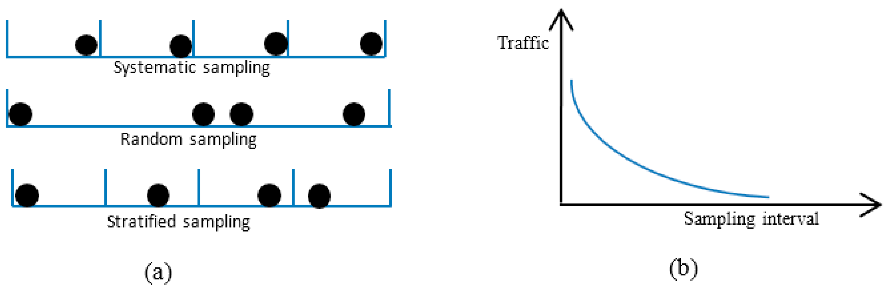
Network Traffic Parameters

The Wireshark network monitoring captured RTP packets (installed on two of the PCs) that were sorted using their sequence numbers to determine end-to-end delay, jitter, and percentage packet loss ratio as outlined below [27,28,29].

End-to-end delay was determined for each packet. For the ith packet, the delay (D_i) was calculated by subtracting the arrival time for the packet ($R_i$) from the sent time ($S_i$) as indicated by Equation (1).

$$D_i=R_i-S_i$$

(1)

The magnitude of jitter (J_i) was measured by determining the difference between the current packet delay ($D_i$) and the delay for the previous packet ($D_{i-1}$) as in Equation (2).

$$J_i=magnitude (D_i-D_{i-1})$$

(2)

The percentage packet loss ratio (%PLR_i) was measured by determining the total number of received packets (${\displaystyle \sum }{R}_i(t)$) and the total number of sent packets (${\displaystyle \sum }{S}_i(t)$) at a given time (t), as illustrated in Equation (3).

$${\%\mathrm{PLR}}_i(t)=\left(1-\frac{{\displaystyle \sum }{R}_i(t)}{{\displaystyle \sum }{S}_i(t)}\right)\times 100$$

(3)

Once the traffic parameters (delay, jitter, and percentage packet loss ratio) were obtained, they were processed by the developed adaptive sampling method. The method used linear regression to model the traffic and the output from the model was interpreted by the fuzzy inference system (FIS) to dynamically adjust the number of packets selected for QoS assessment. The algorithm’s operation is illustrated in the flow chart shown in Figure 4 and related diagram is shown in Figure 5.

The elements of the algorithm are:

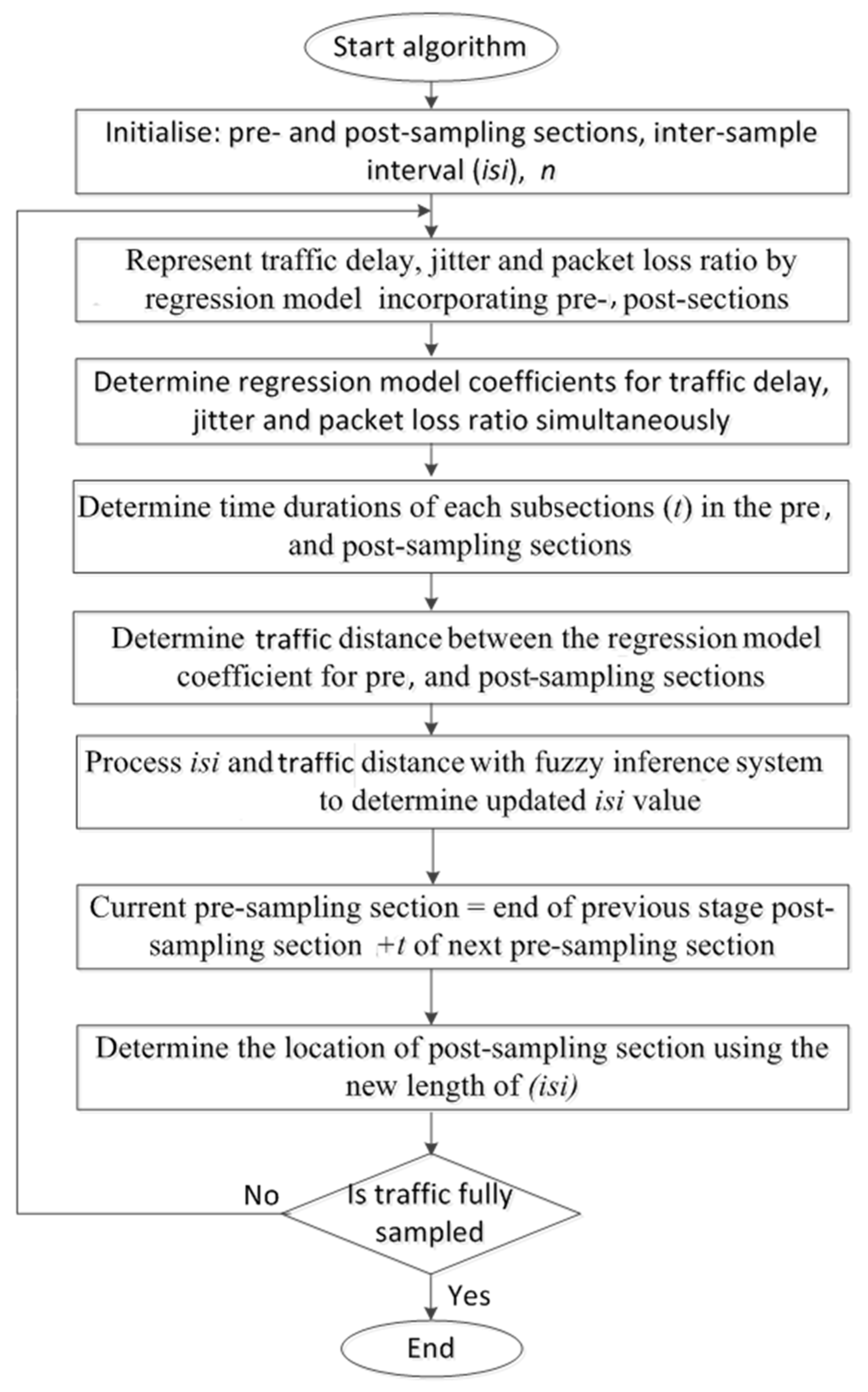
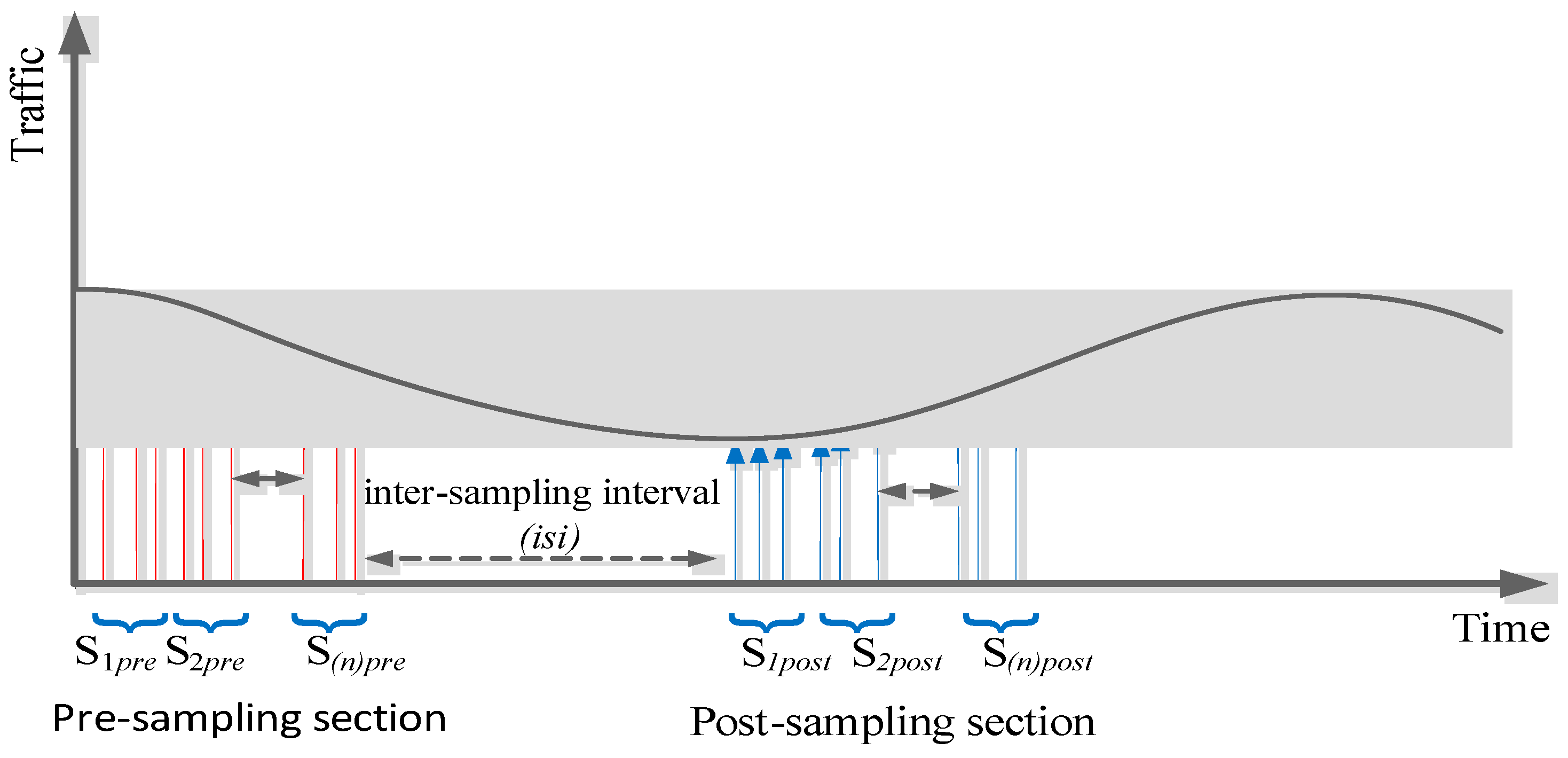
• Pre- and post-sampling sections: These sections contain the traffic that needs to be sampled. The durations of these sections are kept fixed (predefined) and do not change during the sampling process.
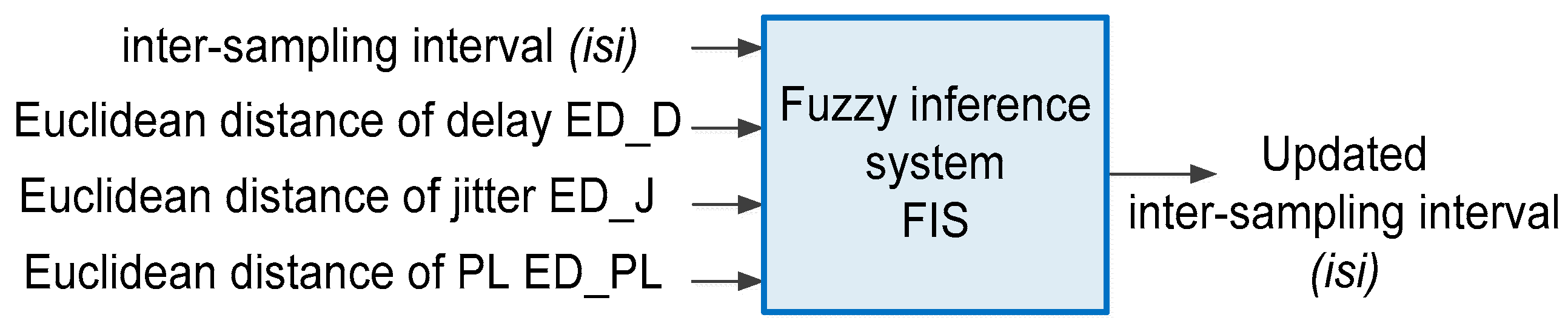
• Inter-section interval (isi): This interval is between the pre- and post-sampling sections. Its duration is adaptively updated by the FIS.
• Regression model: The traffic parameter (i.e., delay, jitter, and percentage packet loss ratio) were represented by an n × n matrix to allow regression analysis, where n is the number of subsections in the pre- and post-sampling sections. Each subsection contained n packets.
• Euclidean distance (ED): ED was used to quantify the extent of traffic variations between the pre- and post-sampling sections.
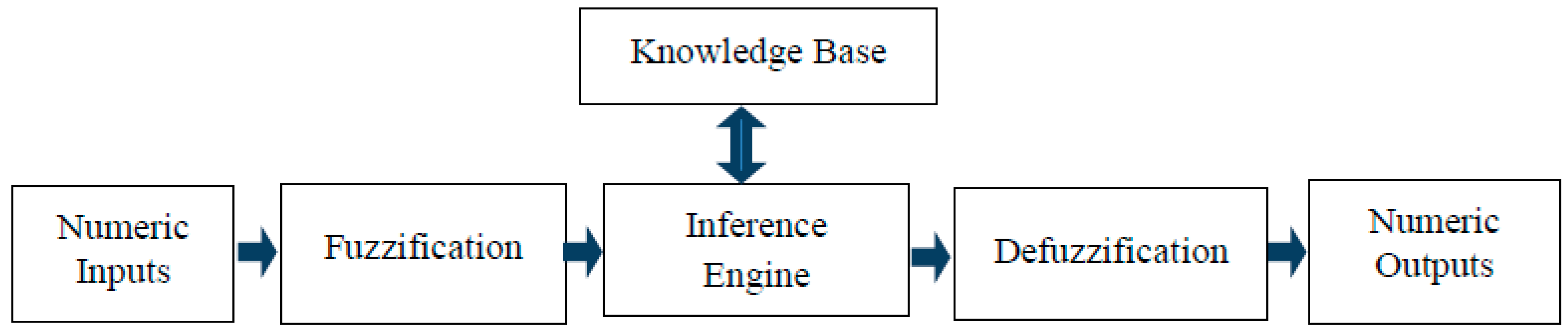
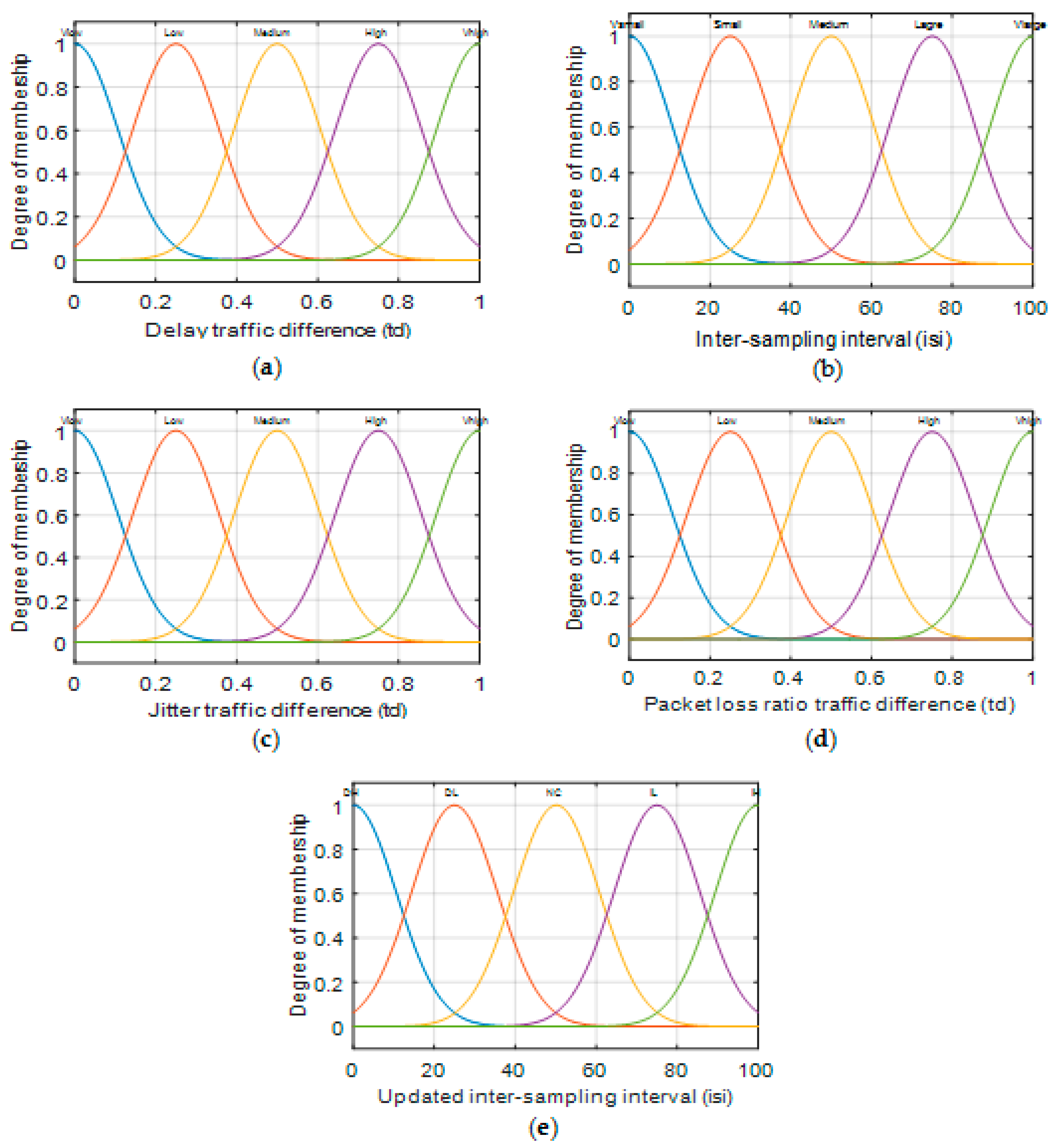
• Fuzzy inference system: FIS was used to update the duration of the isi based on its current value and the ED measures.

The regression model provided the traffic coefficients for the pre- and post-sampling sections. The traffic parameters delay, jitter, and percentage packet loss ratio were considered as the independent variables representing p values in regression Equation (4). The pre- and post-sampling sections were divided into n subsections (s₁, s₂, …, s_n), each subsection containing (n − 1) packets as shown in Figure 5; the traffic values of each subsection were represented by a row of matrix P and the associated time period of every subsection was represented by the vector T as indicated in Equation (4).

In this study, n was chosen as 4, resulting in a 4 × 4 traffic matrix (P). The matrix P, depending on the type of analysis, represented delay values, jitter values, or percentage packet loss ratio values. This generated subsections S₁pre, S₂pre, S₃pre, and S₄pre for the pre-sampling section and S₁post, S₂post, S₃post, and S₄post for the post-sampling section. Each subsection contained 3 data packets. This was repeated for the pre- and post-sampling sections. The general representation of the traffic matrices for pre- and post-sampling sections is shown in Equation (4).

$$T=PC+E=\left[\begin{array}{cccc}1& P_{11}& P_{12}& ‥\\ 1& P_{21}& P_{22}& ‥\\ :& :& :& :\\ 1& P_{n1}& P_{n2}& ‥\end{array}\begin{array}{c}{P}_{1(n-1)}\\ P_{2(n-1)}\\ :\\ P_{n(n-1)}\end{array}\right]\left[\begin{array}{c}{c}_1\\ c_2\\ :\\ c_n\end{array}\right]+\left[\begin{array}{c}{e}_1\\ e_2\\ :\\ e_n\end{array}\right]$$

(4)

The time durations associated with each subsection (s₁, s₂, …, s_n) were represented by t₁, t₂, …, t_n. The vector E = [e₁, e₂, …, e_n] represents the measurement error, assumed to be zero in this study. These durations were measured by subtracting the arrival time of the last packet from the arrival time of first packet in the corresponding subsection. The regression coefficients $c_1,c_2,\dots c_n$ were determined by Equation (5).

$$C=P^{-1}T$$

(5)

The amount of variation in traffic associated with pre- and post-sampling sections was quantified by comparing their respective regression model coefficients using the Euclidean distance, as shown in Equation (6).

$$Euclidean distance=\sqrt{{(c_{1pre}-c_{1post})}^2+{(c_{2pre}-c_{2post})}^2+\dots {(c_{(n)pre}-c_{(n)post})}^2}$$

(6)

FIS received the current duration of the inter-sampling interval (isi) and the Euclidean distance (ED), and then determined the updated value of isi duration as shown in Figure 6.

The Mamdani-type FIS was used to adaptively adjust the length of the isi. Four inputs were fed into the FIS. They were the current inter-sampling interval, and the network parameters delay, jitter, and percentage packet loss ratio. The inputs and the output were fuzzified using the Gaussian membership functions that have a concise notation and are smooth. The Gaussian membership function is represented by the formula expressed in (7) where c_i and σ_i are the mean and standard deviation of the ith fuzzy set A_i [17].

$${\mu }_A{}^i(x)=\exp \left(-\frac{{(c_i-x)}^2}{2{\sigma }_i^2}\right)$$

(7)

The inputs to the fuzzy inference system—the values of traffic Euclidean distance for delay, jitter, and percentage packet loss ratio, and the inter-sampling interval (isi)—were individually fuzzified by five membership functions. The Euclidean distances for delay, jitter, and packet loss were represented by VLow, Medium, High, and VHigh fuzzy sets. The input inter-sampling interval (isi) was represented by VSmall, Small, Medium, Large, and VLarge fuzzy sets. The output was defuzzified by four membership functions, represented by IL (Low Increase), NC (no change), DL (Low Decrease), and DH (High decrease). These membership functions are shown in Figure 7.

Table 1. Mean and standard deviation of the Gaussian fuzzy sets for inputs (Euclidian delay, Euclidian jitter, and Euclidian %PLR).

Membership Functions	(Mean, Standard Deviation (Std)) for ED Delay, ED Jitter, ED of %PLR
Very low	0.1, 0
Low	0.1, 0.25
Medium	0.1, 0.5
High	0.1, 0.75
Very high	0.1, 1

and

Table 2. Mean and standard deviation of the Gaussian fuzzy sets for the inter-sample interval difference and output updated inter-sample interval.

Membership Functions for Current isi	Membership Functions Updated isi	(Mean, Standard Deviation) for Current and Updated isi
Very small	Decrease low (DL)	10, 0
Small	Decrease High (DH)	10, 25
Medium	No change (NC)	10, 50
Large	Increase low (IL)	10, 75
Very large	Increase high (IH)	10, 100

show the mean and standard deviations of the Gaussian membership functions for the fuzzy input sets (i.e., delay, jitter, %PLR, and current isi) and fuzzy output sets (i.e., updated isi), respectively.

The relationship of the inputs, current isi duration, and the Euclidean distance with the output (i.e., updated isi duration) was represented by twenty rules, as shown in

Table 3. Rules included in the FIS knowledge base (TD is time difference).

Rule	Current isi	TD Delay	TD Jitter	TD Packet Loss Ratio	Updated isi
1	Very small	Very low	Very low	None	Increase high (IH)
2	Very small	Very low	None	Very low	Increase high (IH)
3	Very small	None	Very low	Very low	Increase high (IH)
4	None	Very low	Very low	Very low	Increase high (IH)
5	None	Low	Low	Low	Increase low (IL)
6	Small	None	Low	Low	Increase low (IL)
7	Small	Low	None	Low	Increase low (IL)
8	Small	Low	Low	None	Increase low (IL)
9	Medium	Medium	Medium	None	No change (NC)
10	Medium	Medium	None	Medium	No change (NC)
11	Medium	None	Medium	Medium	No change (NC)
12	None	Medium	Medium	Medium	No change (NC)
13	None	High	High	High	Decrease low (DL)
14	Large	None	High	High	Decrease low (DL)
15	Large	High	None	High	Decrease low (DL)
16	Large	High	High	None	Decrease low (DL)
17	None	Very high	Very high	Very high	Decrease low (DH)
18	Very large	None	Very high	Very high	Decrease low (DH)
19	Very large	Very high	None	Very high	Decrease High (DH)
20	Very large	Very high	Very high	None	Decrease High (DH)

.

The inputs to the FIS, i.e., the ED and current inter-sample interval, were fuzzified using three membership functions. The ED was represented by Low, Medium, and High fuzzy sets and the current inter-sample interval (isi) was represented by Small, Medium, and Large fuzzy sets. The output was defuzzified by four membership functions, represented as IL (low increase), NC (no change), DL (low decrease), and DH (high decrease). These membership functions are shown in Figure 7.

To evaluate the effectiveness of the developed adaptive sampling method, comparisons of the original traffic’s data packets and its sampled versions were carried out. Comparisons of mean and standard deviation of the sampled packets to those of its original populations may not be enough to evaluate the accuracy of the sampled version in terms of demonstrating the original population as they can be obscured by outliers [30,31]. Therefore, additional evaluations were used to assess the efficiency of the developed sampling approach. The bias indicates how far the mean of the sampled data lies from the mean of its original population [31]. Bias is the average of difference of all samples of the same size. The bias was calculated as in Equation (10):

$$\mathrm{Bias}=\frac{1}{N}{\displaystyle \sum _{i=1}^N{M}_i-M}$$

(10)

where N is the number of simulation runs, and M_i and M are the means of the traffic parameters for the original data and its sampled population.

The Relative Standard Error (RSE) is another parameter that can be used to assess the accuracy and efficiency of the technique—RSE examines the reliability of sampling [13]. RSE is defined as a percentage and can be defined as the standard error of the sample (SE) divided by the sample size (n), as in Equation (11):

$$\mathrm{RSE}=\frac{\mathrm{SE}}{n}\times 100$$

(11)

where n is the sample size, and SE is the standard error values of the original and sampled data population.

Curve fitting is another measurement method that has been used to demonstrate the behaviour of the sampled data version in terms of representing the original data population. It examines the trends of the sampled data version and its equivalent original data by applying the curve fitting approach. Curve fitting is a suitable tool for representing a data set in linear, quadratic, or polynomial forms [32] [33]. Data curve fitting is based on two functions—the polynomial evaluation function and the polynomial curve fitting function. The general formula for a polynomial is shown in Equation (12).

$$f(x)=a_0{x}^N+a_1{x}^{N-1}+a_2{x}^{N-2}+\dots \dots +a_{N-1}{x}^{}+a_N$$

(12)

The polynomial curve fitting function measures a least squares polynomial for a given data set of x and generates the coefficients of the polynomial which can be used to illustrate a curve to fit the data according to the specified degree (N). The degree of a polynomial is equal to the maximum value of the exponents (N), and [a₀ … a_N] is a set of polynomial coefficients. The polynomial evaluation function examines a polynomial for x values and then produces a curve to fit the data based on the coefficients that were found using the curve fitting function [32,33].

The sampling fraction is the proportion of a population that will be counted. Sampling fraction is the ratio of the sampled size (n) divided by the population size. In this study, the curve fitting results have been marked by a red color to demonstrate original and sampled data trends.

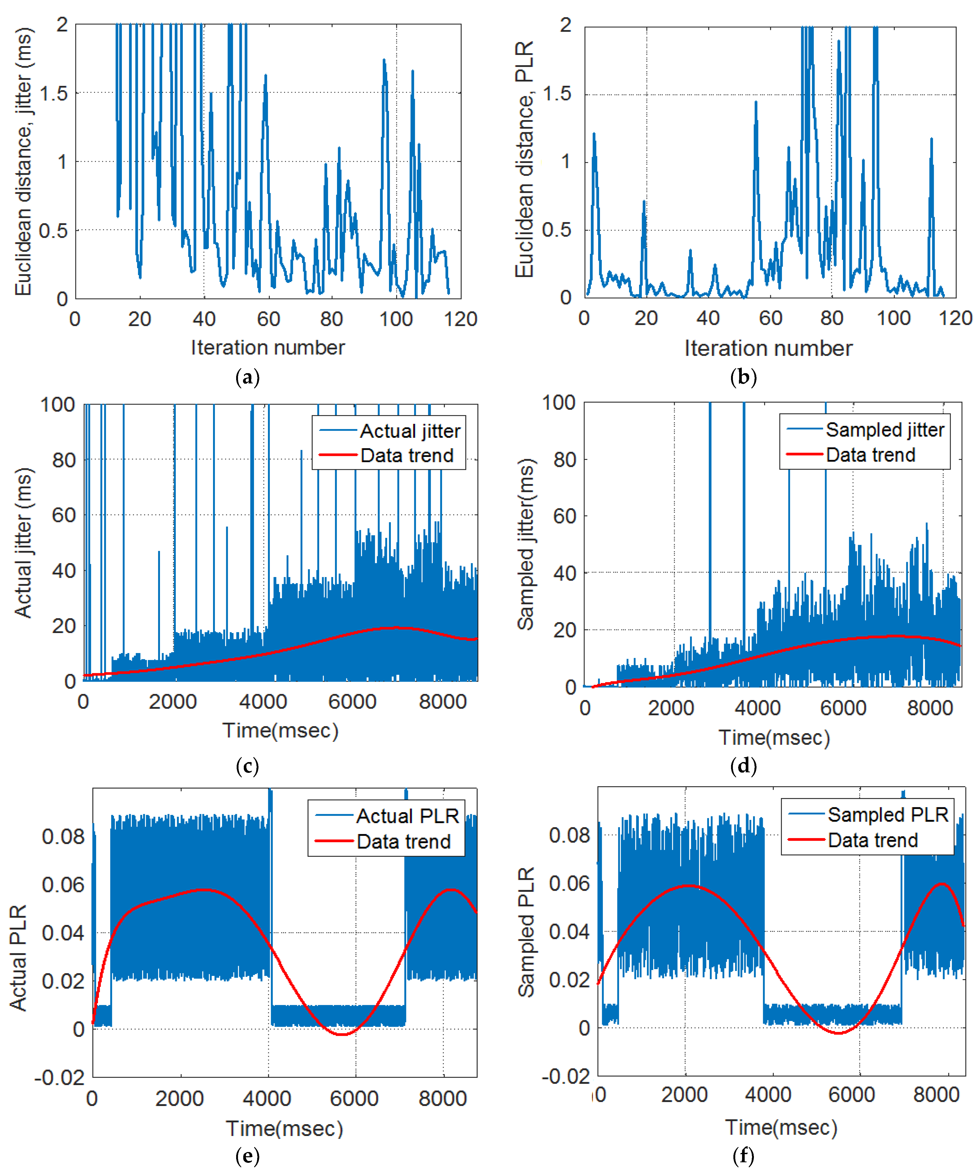
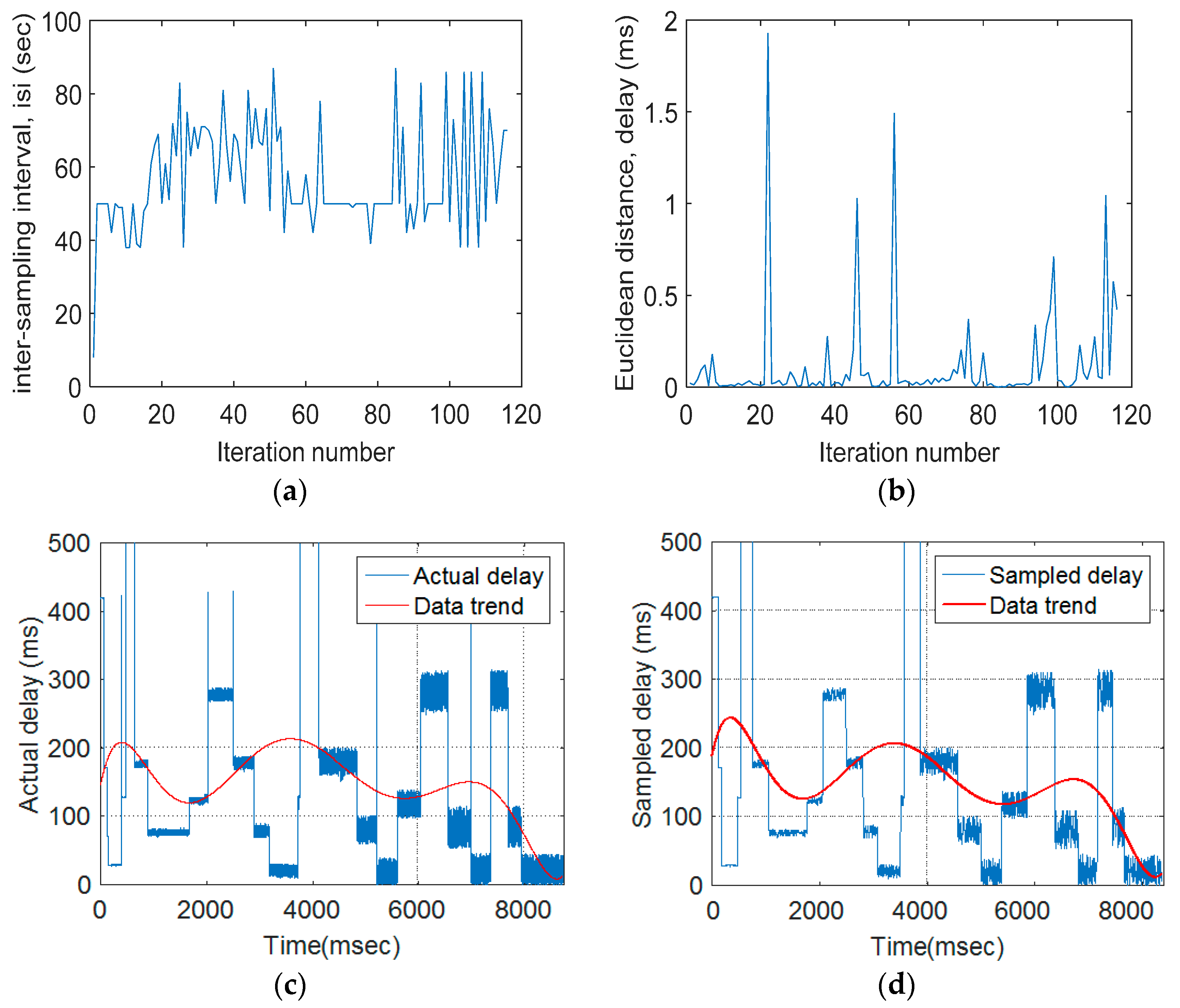
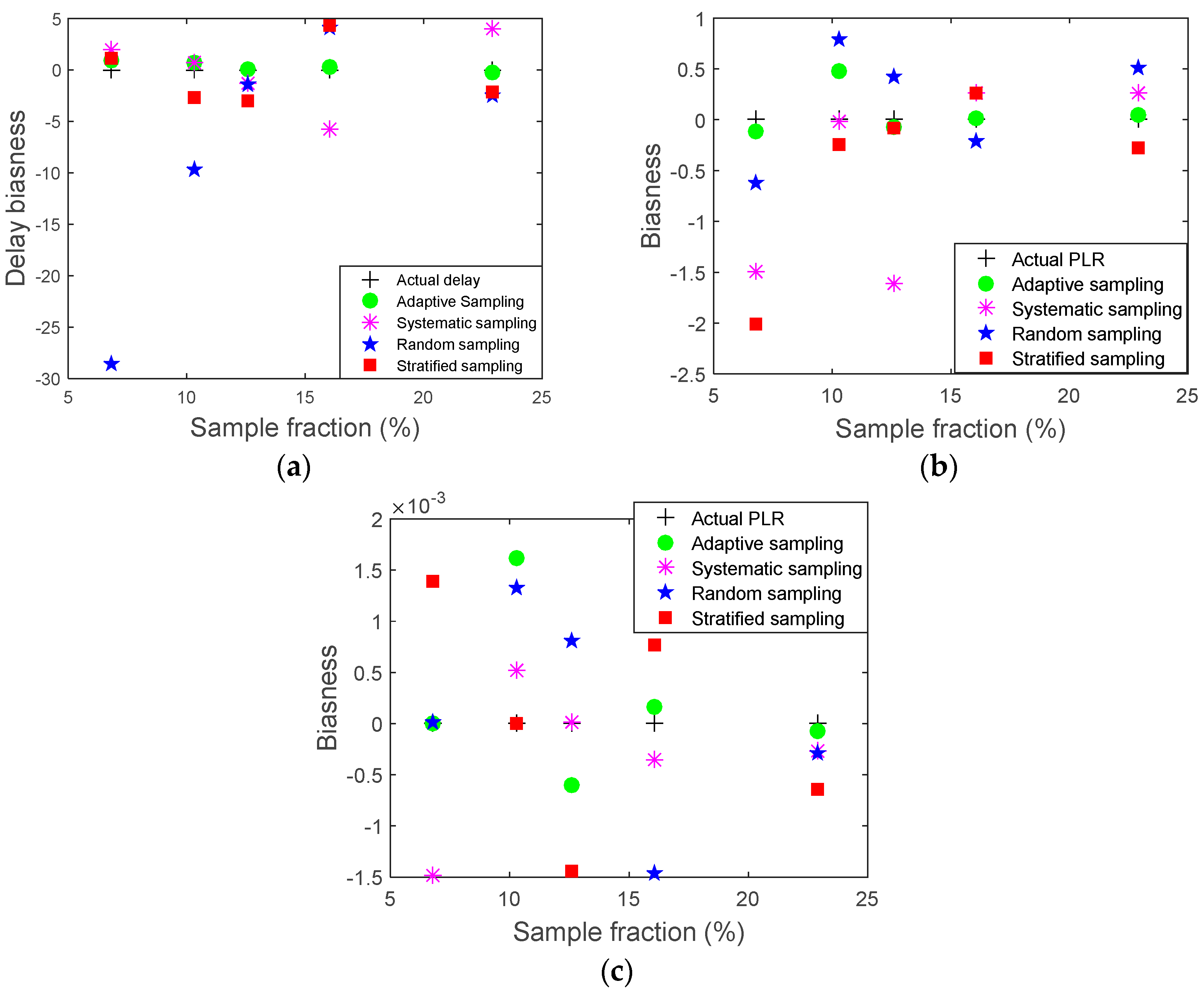
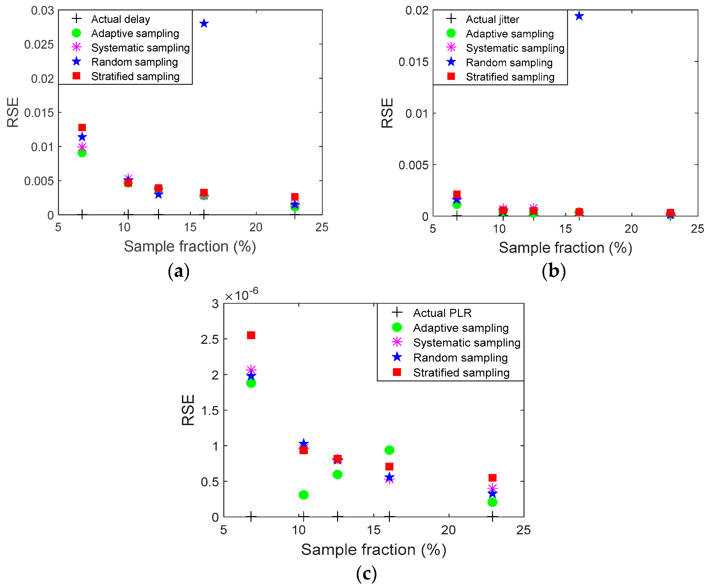
3. Results and Discussion

The traffic consisting of packets for different applications were captured and their parameters, i.e., delay, jitter, and percentage packet loss ratio, were determined using Equations (1)–(3). The simulation duration was up to three minutes. The linear regression Equations (4) and (5) were used to model the traffic. The Euclidean distance (ED) shown in Equation (6) was used to quantify the variation in the behaviour of the traffic associated with the pre- and post-sampling sections. The FIS output indicated the updated isi duration for each iteration, based on the values of the FIS inputs and the fuzzy rules. As an example, Figure 8a indicates the adaptive updating of isi based on the variations in packet delay. Figure 8b indicates the manner in which the Euclidean distance and the variation of Euclidean distances of delay, jitter, and packet loss ratio affect isi changes. When traffic variations were large, isi decreased and vice versa. Figure 8c shows the original delay and its trend and Figure 8d indicates the sampled delay and its trend. The trends for the original delay and its sampled version are close. In Figure 8c–e the curve fitting method has been used for both the original and sampled versions of the traffic parameters; the fitted curve shown in red indicates the data trend for the original population and the sampled version. The trend of the sampled version using the adaptive sampling technique represents the original data closely.

Figure 9a–d indicate the manner in which the developed adaptive sampling method represented the jitter and percentage packet loss ratio (%PLR). Figure 9a,b show the Euclidean distance measures. The Euclidean distance of the packet loss ratio variation changed more than the variations of delay and jitter due to rapid changes in the packet loss ratio; these variations in the Euclidean distance caused the changes in the isi values. Figure 9c–f show the actual (original) jitter and %PLR and their respective sampled versions. For both traffic parameters, the trends for the original traffic parameters were close to those of the sampled versions.

Table 4. Measurement results for delay using different sampling methods: adaptive, systematic, random, and stratified.

Unit	Sample Fractions %
	0	6.1	10.2	13	22.9
Adaptive sampling method
Mean	146	147	147	147	147
Std.	141	141	141	142	141
Bias	0	0.875	0.683	0.067	−0.262
RSE	0	0.0090	0.0040	0.0030	0.0011
Systematic sampling
Mean	147	145	146	148	143
Std.	141	146	142	141	138
Bias	0	1.9740	0.725	−1.279	3.960
RSE	0	0.0099	0.0052	0.0038	0.0019
Random sampling
Mean	147	176	157	149	150
Std.	141	165	152	149	142
Bias	0	−28.551	−9.741	−1.401	−2.432
RSE	0	0.0113	0.0050	0.0029	0.0014
Stratified sampling
Mean	147	146	150	150	149
Std.	141	143	149	142	139
Bias	0	1.0932	−2.74034	−2.9770	−2.1844
RSE	0	0.0127	0.0046	0.00389	0.00265

Std.: standard deviation.

provides a summary of delay sampling results for the original traffic (0% sample fraction) and a number of different sample fractions for the adaptive and nonadaptive sampling methods of systematic, random, and stratified sampling methods. Similar information is provided for jitter and %PLR in

Table 5. Measurement results of jitter using different sampling methods: adaptive, systematic, random, and stratified.

Unit	Sample Fractions %
	0.0	6.1	10.2	13	22.9
Adaptive sampling method
Mean	11.116	11.235	10.6386	11.1855	11.0730
Std.	17.493	17.479	11.636	14.073	17.4936
Bias	0	−0.1185	0.478	−0.0689	0.0435
RSE	0	0.00112	4.31 × 10−4	2.69 × 10−4	1.5 × 10−4
Systematic sampling
Mean	11.116	12.6123	11.133	12.732	10.855
Std.	17.493	23.7784	21.049	26.650	12.120
Bias	0	−1.4956	−0.016	−1.615	0.261
RSE	0	0.00161	6.97 × 10−4	7.40 × 10−4	1.66 × 10−4
Random sampling
Mean	11.116	11.733	10.325	10.691	10.608
Std.	17.493	23.990	13.723	21.510	14.770
Bias	0	−0.6166	0.790	0.425	0.508
RSE	0	0.00165	4.53 × 10−4	4.34 × 10−4	1.55 × 10−4
Stratified sampling
Mean	11.116	13.127	11.357	11.202	11.389
Std.	17.493	23.601	19.236	18.428	18.681
Bias	0	−2.011	−0.241	−0.085	−0.272
RSE	0	0.002	6.08 × 10−4	5.05 × 10−4	3.5 × 10−4

and

Table 6. Measurement results of packet loss ratio using different sampling methods: adaptive, systematic, random, and stratified.

Unit	Sample Fractions %
	0.0	6.1	10.2	13	22.9
Adaptive sampling method
Mean	0.0356	0.035	0.034	0.036	0.035
Std.	0.0291	0.0292	0.0290	0.029	0.029
Bias	0	6.23 × 10−6	0.0016	−5.96 × 10−4	−7.22 × 10−5
RSE	0	1.88 × 10−6	3.05 × 10−7	5.93 × 10−7	2.08 × 10−7
Systematic sampling
Mean	0.0356	0.037	0.035	0.035	0.035
Std.	0.0291	0.029	0.0290	0.028	0.029
Bias	0	−0.0014	5.20 × 10−4	7.95 × 10−6	−2.72 × 10−4
RSE	0	2.06 × 10−6	9.62 × 10−7	8.05 × 10−7	3.99 × 10−7
Random sampling
Mean	0.0356	0.035	0.0343	0.034	0.035
Std.	0.0291	0.029	0.027877	0.028954	0.029492
Bias	0	1.65 × 10−5	0.0013	8.07 × 10−4	−2.90 × 10−4
RSE	0	1.98 × 10−6	1.03 × 10−6	7.94 × 10−7	3.30 × 10−7
Stratified sampling
Mean	0.0356	0.034	0.035	0.037	0.036
Std.	0.0291	0.028	0.029	0.029	0.0286
Bias	0	0.0013	1.03 × 10−6	−0.0014	−6.45 × 10−4
RSE	0	2.55 × 10−6	9.35 × 10−7	8.13 × 10−7	5.47 × 10−7

. To compare the developed adaptive sampling and nonadaptive sampling methods, the bias and relative standard errors (RSE) were determined. They indicated that the developed adaptive method has the lowest relative error and bias values in most of the sample fractions as compared as compared with the nonadaptive methods, signifying an improved performance.

Table 6 shows the difference in representation of the actual delay at different sample fractions using adaptive and nonadaptive sampling methods. For all used sampling techniques, as the sample size increased, the deviation of sampled mean, standard deviation from the actual mean, and standard deviation decreased accordingly. This is because a large sample size contains a larger number of packets that, in turn, increases the probability of representing original data more accurately. The mean and standard deviation of the original delay population were 146 ms and 141 ms, respectively, whereas the sampled delay population obtained from the adaptive sampling method had a mean of 147 ms and standard deviation of 141 ms, respectively, at 22.9% sample fraction. However, the mean and standard deviation of the original data population of sampled delay using systematic, random, and stratified sampling were 143 ms, 150 ms, and 149 ms and 138 ms, 142 ms, and 139 ms, respectively. These indicate that the delay values of sampled versions by the adaptive sampling technique represented the original delay more accurately.

The results indicate a similar trend for jitter, as indicated in Table 5. The mean and standard deviation of the original jitter population were 11.116 ms and 17.493 ms, respectively, whereas the sampled jitter population obtained from the adaptive sampling method had a mean of 11.073 ms and standard deviation of 17.494 ms, respectively, at a 22.9% sample fraction. However, the mean and standard deviation of original data population of sampled jitter using systematic, random, and stratified sampling were 10.855 ms, 10.608 ms, and 11.389 ms and 12.120 ms, 14.770 ms, and 18.681 ms, respectively. This indicates that the jitter for sampled versions using the adaptive sampling technique represented the original jitter more accurately.

Table 6 indicates a similar trend for %PLR. The mean and standard deviation of the original %PLR population were 0.0356 and 0.0291, respectively, whereas the sampled %PLR population obtained from the adaptive sampling method had a mean of 0.035 and standard deviation of 0.029, respectively, at a 22.9% sample fraction. However, the mean and standard deviation of the original data population of sampled %PLR using systematic, random, and stratified sampling were 0.035, 0.035, and 0.036 and 0.029, 0.0294, and 0.0286, respectively. This specifies that the %PLR sampled versions by the adaptive sampling technique represented the original PLR more accurately.

Figure 10a–c show, respectively, comparisons of the bias of sampled delay, jitter, and %PLR for different sample fractions using the proposed adaptive sampling method and nonadaptive sampling methods of systematic, random, and stratified.

In Figure 11a–c, the RSE for the sampled delay, jitter, and %PLR for nonadaptive sampling approaches (systematic, random, and stratified) are compared with the measured RSE for the proposed adaptive sampling method. The results indicate that the proposed adaptive sampling method has a lower RSE as compared with the nonadaptive sampling approaches. For example, at a 22.97% sample fraction, the RSE of the sampled delay was 0.0011, while the bias values for systematic, stratified, and random sampling were 0.0019, 0.0014, and 0.00265, respectively. The results demonstrate that the adaptive sampling approach has the lowest RSE compared with nonadaptive sampling methods. RSE values decreased and became closer to zero for all methods when sample size increased.

The results indicate that the bias decreased and became closer to zero for all sampling methods when the sample size increased. Furthermore, the proposed adaptive sampling method has a lower bias as compared with systematic, stratified, and random sampling approaches. For example, at 22.9% sample fraction, the bias of sampled delay was −0.262, while the bias values for systematic, random, and stratified sampling were 3.960, −2.432, and −2.1844, respectively. When the sample fraction was the lowest value, i.e., 6.1%, the smallest bias was for the developed adaptive method with 0.875, followed by the stratified sampling method with 1.093, then systematic methods with 1.974; the highest bias was for the random method at −28.55.

The higher performance of adaptive sampling over conventional nonadaptive sampling is due to the selection of packets considering the traffic variations, whereas the packet selection in the nonadaptive approaches depended either on a predefined or random manner.

4. Conclusions

A novel adaptive technique that samples computer network traffic has been developed and its performance has been compared with that of the nonadaptive sampling methods of random, stratified, and systematic sampling. The developed method adaptively adjusted a section called the inter-sampling interval, resulting in an increase in sampling when the traffic variations were greater and vice versa. The developed adaptive sampling represented the original traffic more closely than did the nonadaptive sampling. The developed adaptive method was successfully applied to a physical computer network and showed better performance. The developed adaptive sampling method can be valuable for evaluating multimedia network performance.

The developed adaptive sampling can particularly be applied for traffic analysis of healthcare networks, as the management and support provided to patients increasingly rely on multimedia-type applications.

References

1. Lazakidou, A.; IIiopoulou, D. Useful applications of computers and smart mobile technologies in the health sector. J. Appl. Med. Sci. 2012, 1, 27–60. [Google Scholar]
2. Robitza, W.; Ahmad, A.; Kara, P.A.; Atzori, L.; Martini, M.G.; Raake, A.; Sun, L. Challenges of future multimedia QoE monitoring for internet service providers. Multimed. Tools Appl. 2017, 76. [Google Scholar] [CrossRef]
3. Rodíguez, M.A.V.; Muñoz, E.C. Review of quality of service (QoS) mechanisms over IP multimedia subsystems (IMS). Ing. Desarro. 2017, 35, 262–281. [Google Scholar] [CrossRef]
4. Wesseler, M.; Saatchi, R.; Burke, D. Child-friendly wireless remote health monitoring system. In Proceedings of the IEEE 9th International Symposium on Communication Systems, Networks and Digital Signal Processing, Manchester, UK, 23–25 July 2014; pp. 198–202. [Google Scholar]
5. Clarke, A.; Steele, R. Health participatory sensing networks. Mob. Inf. Syst. 2014, 10, 229–242. [Google Scholar] [CrossRef]
6. González, F.C.J.; Villegas, O.O.V.; Ramírez, D.E.T.; Sánchez, V.G.C.; Domínguez, H.O. Smart multi-level tool for remote patient monitoring based on a wireless sensor network and mobile augmented reality. Sensors 2014, 14, 17212–17232. [Google Scholar] [CrossRef] [PubMed]
7. Ghamari, M.; Janko, B.; Sherratt, R.S.; Harwin, W.; Piechockic, R.; Soltanpour, C. A survey on wireless body area networks for eHealthcare systems in residential environments. Sensors 2016, 16, 831. [Google Scholar] [CrossRef] [PubMed]
8. Van Halteren, A.; Bults, R.; Wac, K.; Dokovsky, N.; Koprinkov, G.; Widya, I.; Konstantas, D.; Jones, V. Wireless body area networks for healthcare: The mobiHealth project. Stud. Health Technol. Inform. 2004, 108, 121–126. [Google Scholar]
9. Varshney, U.; Sneha, S. Patient monitoring using ad hoc wireless networks: Reliability and power management. IEEE Commun. Mag. 2006, 44, 49–55. [Google Scholar] [CrossRef]
10. Manfredi, S. Performance evaluation of healthcare monitoring system over heterogeneous wireless networks. E-Health Telecommun. Syst. Netw. 2012, 1, 27–36. [Google Scholar] [CrossRef]
11. Lin, R.; Li, O.; Li, Q.; Dai, K. Exploring adaptive packet-sampling measurements for multimedia traffic classification. J. Commun. 2014, 9, 971–979. [Google Scholar]
12. Salama, A.; Saatchi, R.; Burke, D. Quality of Service Evaluation and Assessment Methods in Wireless Networks. In Proceedings of the 4th International Conference on Information and Communication Technologies for Disaster Management, Munster, Germany, 11–13 December 2017. [Google Scholar]
13. AL-Sbou, Y.A.; Saatchi, R.; Al-Kyayatt, S.; Ayyash, M.; Saraireh, M. A novel quality of service assessment of multimedia traffic over wireless ad hoc networks. In Proceedings of the 2nd International Conference on Next Generation Mobile Applications, Services and Technologies, Cardiff, UK, 16–19 September 2008; pp. 479–484. [Google Scholar]
14. Silva, J.M.C.; Paulo, C.; Solange, R.L. Inside packet sampling techniques: Exploring modularity to enhance network measurements. Int. J. Commun. Syst. 2017, 30. [Google Scholar] [CrossRef]
15. Bělohlávek, R.; George, J.K.; Dauben, J.W. Fuzzy Logic and Mathematics: A Historical Perspective; Oxford University Press: Oxford, UK, 2017. [Google Scholar]
16. Yuste, A.J.; Triviño, A.; Casilari, E. Using fuzzy logic in hybrid multihop wireless networks. Int. J. Wirel. Mobil. Netw. 2010, 2, 96–108. [Google Scholar] [CrossRef]
17. Ross, T.J. Fuzzy Logic with Engineering Applications, 4th ed.; Wiley: Hoboken, NJ, USA, 2017. [Google Scholar]
18. Dogman, A.; Saatchi, R.; Al-Khayatt, S.; Nwaizu, H. Adaptive statistical sampling of VoIP traffic in WLAN and wired networks using fuzzy inference system. In Proceedings of the 2011 7th International Wireless Communications and Mobile Computing Conference, Istanbul, Turkey, 4–8 July 2011; pp. 1731–1736. [Google Scholar]
19. Dogman, A.; Saatchi, R.; Al-Khayatt, S. An adaptive statistical sampling technique for computer network traffic. In Proceedings of the 7th International Symposium on Communication Systems Networks and Digital Signal Processing (CSNDSP), Newcastle upon Tyne, UK, 21–23 July 2010; IEEE: Piscataway, NJ, USA, 2010; pp. 479–483. [Google Scholar]
20. Fan, J.; Liao, Y.; Liu, H. An overview of the estimation of large covariance and precision matrices. Econom. J. 2016, 19, C1–C32. [Google Scholar] [CrossRef]
21. Faraway, J.J. Extending the Linear Model with R: Generalized Linear, Mixed Effects and Nonparametric Regression Models; CRC Press: Boca Raton, FL, USA, 2016; Volume 124. [Google Scholar]
22. Zhang, B.; Liu, Y.; He, J.; Zou, Z. An energy efficient sampling method through joint linear regression and compressive sensing. In Proceedings of the 2013 Fourth International Conference on Intelligent Control and Information Processing (ICICIP), Beijing, China, 9–11 June 2013; IEEE: Piscataway, NJ, USA, 2013; pp. 447–450. [Google Scholar]
23. Pacheco de Carvalho, J.A.R.; Veiga, H.; Ribeiro Pacheco, C.F.; Reis, A.D. Performance evaluation of IEEE 802.11 a, g laboratory open point-to-multipoint links. In Proceedings of the World Congress on Engineering (WCE), London, UK, 1–3 July 2015; Volume 1. [Google Scholar]
24. Sanders, C. Practical Packet Analysis: Using Wireshark to Solve Real-World Network Problems; No Starch Press: San Francisco, CA, USA, 2017. [Google Scholar]
25. Yohannes, D.; Dilip, M. Effect of delay, packet loss, packet duplication and packet reordering on voice communication quality over WLAN. TECHNIA 2016, 8, 1071–1075. [Google Scholar]
26. Salama, A.; Saatchi, R.; Burke, D. Adaptive sampling technique for computer network traffic parameters using a combination of fuzzy system and regression model. In Proceedings of the 2017 4th International Conference on Mathematics and Computers in Science in Industry (MCSI 2017), Corfu Island, Greece, 24–26 August 2017; IEEE: Piscataway, NJ, USA, 2017. [Google Scholar]
27. Salama, A.; Saatchi, R.; Burke, D. Adaptive sampling technique using regression modelling and fuzzy inference system for network traffic. In Harnessing the Power of Technology to Improve Lives; Cudd, P., De Witte, L., Eds.; Studies in Health Technology and Informatics (242); IOS Press: Amsterdam, The Netherlands, 2017; pp. 592–599. [Google Scholar]
28. Salama, A.; Saatchi, R.; Burke, D. Adaptive sampling for QoS traffic parameters using fuzzy system and regression model. Math. Model. Methods Appl. Sci. 2017, 11, 212–220. [Google Scholar]
29. Saraireh, M.; Saatchi, R.; Al-Khayatt, S.; Strachan, R. Assessment and improvement of quality of service in wireless networks using and hybrid genetic-fuzzy approaches, Artif. Intell. Rev. 2007, 27, 95–111. [Google Scholar] [CrossRef]
30. Zseby, T. Comparison of sampling methods for non-intrusive SLA validation. In Proceedings of the Second Workshop on End-to-End Monitoring Techniques and Services (E2EMon), San Diego, CA, USA, 3 October 2004. [Google Scholar]
31. Wan, X.; Li, Y.; Xia, C.; Wu, M.; Liang, J.; Wang, N. A T-wave alternans assessment method based on least squares curve fitting technique. Measurement 2016, 86, 93–100. [Google Scholar] [CrossRef]
32. Guruswami, V.; Zuckerman, D. Robust Fourier and polynomial curve fitting. In Proceedings of the 2016 IEEE 57th Annual Symposium on Foundations of Computer Science (FOCS), New Brunswick, NJ, USA, 9–11 October 2016; IEEE: Piscataway, NJ, USA, 2016. [Google Scholar]
33. Lindfield, G.; Penny, J. Numerical Methods: Using MATLAB; Academic Press: Cambridge, MA, USA, 2012. [Google Scholar]
Figure 1. An illustration of sampling techniques: (a) Nonadaptive sampling; (b) The concept of adaptive sampling [12].
Technologies 06 00024 g001
Figure 2. The fuzzy inference system.
Technologies 06 00024 g002
Figure 3. The network topology used in the study.
Technologies 06 00024 g003
Figure 4. The flow chart of the adaptive sampling algorithm.
Technologies 06 00024 g004
Figure 5. Traffic representations for the regression model.
Technologies 06 00024 g005
Figure 6. Fuzzy system to update isi duration.
Technologies 06 00024 g006
Figure 7. Membership functions for (ac) the Euclidean distance sets for delay, jitter, and percentage packet loss ratio; (d) inter-sampling interval; and (e) the updated inter-sampling interval.
Technologies 06 00024 g007
Figure 8. Typical results obtained from the developed adaptive technique: (a) FIS output for the inter-sampling interval (isi), (b) the Euclidean distance for delay, (c) original traffic delay, and (d) sampled traffic delay.
Technologies 06 00024 g008
Figure 9. Typical results obtained from the developed adaptive technique: (a) measured Euclidean distance for jitter, (b) measured Euclidean distance for packet loss, (c) original traffic jitter, (d) sampled traffic percentage jitter, (e) original traffic packet loss ratio, and (f) sampled traffic packet loss ratio.
Technologies 06 00024 g009
Figure 10. Comparisons of biasness of (a) delay, (b) jitter, and (c) %PLR between the developed technique and nonadaptive methods.
Technologies 06 00024 g010
Figure 11. Comparisons of RSE of (a) delay, (b) jitter, and (c) PLR between the developed technique and nonadaptive methods.
Technologies 06 00024 g011