A Robust Tunable Simulator of Atmospheric Turbulence for Performance Analysis of Wireless Optical Links

Abstract

Atmospheric turbulence distorts the wavefront of propagating optical radiation, degrading image resolution in astronomical telescopes and reducing power density at the target in focusing applications. These effects can be studied under controlled laboratory conditions using turbulence-generating devices—such as fan heaters (rough control), phase plates, or active mirrors (fine control)—in combination with a wavefront sensor for measurements. To support this research, we developed a software simulator for reconstructing atmospheric phase fluctuations. The integrated software–hardware system can generate phase screens following Kolmogorov turbulence statistics, incorporating parameters for wind velocity and the D/r₀ ratio. Phase screens were produced with an average approximation error of 0.01 µm (less than 5%). The average reconstruction error was 0.017 µm, corresponding to approximately 8%. The newly developed phase screen simulator outperforms the fastest existing version in several key aspects. Its aperture size is doubled, increasing from 400 mm to 800 mm, while the phase screen generation resolution expands by half, from 700 × 700 pixels to 1024 × 1024 pixels. The operating wavelength range also broadens significantly—from a maximum of 2.2 µm in the existing tool to 10 µm in the new one. Additionally, the wind velocity range becomes 1.5 times wider, extending from 30 m/s to 50 m/s. The developed tool might be useful for the performance analysis of wireless links, particularly in the estimation of bit error rate and quantum efficiency using the wavefront root mean square error.

1. Introduction

1.1. Background and Related Works

Atmospheric turbulence [1,2,3] causes random fluctuations in the refractive index of air [4], distorting the wavefronts of optical radiation propagating through the atmosphere [5]. This phenomenon fundamentally limits ground-based astronomy by degrading image resolution [6,7,8] and reduces the spatial coherence of laser systems [9,10,11,12]. The scientific community has extensively investigated this phenomenon. Lukin et al. developed an approximate spectrum model for coherent turbulence, calculated optical image jitter variance, and demonstrated that phase fluctuations decrease significantly in coherent turbulence [13]. Qin and Liao employed clean numerical simulation to solve 3D turbulent Kolmogorov flow and found that direct numerical simulation results are quickly polluted by numerical noise, deviating substantially from the clean numerical simulation benchmark solution in spatial symmetry, energy cascade, and statistical properties [14]. Guzev et al. performed direct numerical modeling of viscous weakly compressible Kolmogorov-type flows and proposed a rank analysis of vorticity, energy, and pressure distributions, identifying the inflection point in rank frequency distributions as a universal flow classification characteristic [15].

Atmospheric turbulence severely affects free-space optical (FSO) transmission applications, including wireless power delivery to remote sites, aerial platforms [16,17], low-earth-orbit satellites [18], secure optical communication links [19], and precise beam control for laser cutting, material processing, and optical data recording [20,21]. Directed-energy applications, such as neutralizing unmanned aerial vehicles or mitigating space debris [22,23,24], are also compromised by turbulence-induced beam wander and spreading. System efficiency is constrained by beam diffraction [25,26,27,28], aerosol scattering [29,30,31,32,33,34,35], and, most critically, dynamic phase distortions from atmospheric turbulence [36,37,38,39]. Therefore, restoring wavefront quality is essential for extending the operational range and reliability of such systems, a problem that has motivated decades of ongoing research [40,41,42,43,44].

The universal energy cascade described by the turbulent energy spectrum provides the theoretical foundation for turbulence modeling and simulation. Accurate reproduction of this energy distribution is essential for any valid simulation approach. Before deploying complex adaptive optics systems in the field, controlled laboratory replication of turbulence-induced optical effects enables the systematic investigation of beam propagation [45,46] and the rigorous testing of compensation strategies.

Beason et al. developed an in-air laboratory turbulence generator based on water tank concepts [47]. Mao et al. introduced a Mie-scattering lidar method to detect atmospheric turbulence intensity by extracting light intensity fluctuations from return signals to obtain the refractive index structure constant $C_n^2$ [48]. Kolb et al. developed and tested the MAPS turbulence generator for MCAO [49]. This generator had limited wavelength and atmospheric path range, and a set of discrete wind speed values. Sriram and Kearney improved phase screen generation performance by 60 times using linear and statistical properties [50]. However, their simulator had limited phase screen resolution (200 × 200 pixels only). Rinker created an open-source tool for simulating turbulence boxes constrained by measured data, useful for wind turbine model validation [51]. Richards et al. developed a GPU-based fast turbulence generator achieving 4-to-75 times faster performance compared to CPU implementations [52]. The simulator developed by Richards et al. also suffered from a small phase screen resolution (up to 256 pixels) yet demonstrated good performance results due to the GPU acceleration. Wilcox et al. developed a testbed for atmospheric turbulence simulation using Kolmogorov statistics to test adaptive optical system correctability with spatial light modulators (SLM) [53]. This tool is probably the best to date; however, it also suffers from a small wavelength range and, in general, has a limited set of parameters that can be adjusted by the user.

Despite extensive research on turbulence simulation over decades, existing approaches exhibit several critical limitations:

• Insufficient phase screen resolution;
• Low phase screen generation frequency;
• Hardware dependencies (requiring GPUs or high-end CPUs);
• Restricted parameter ranges for wavelength, wind speed, and path length.

1.2. Research Novelty

To address these limitations, this research presents the development and experimental validation of a dedicated hardware–software turbulence simulator based on the thin phase screen approximation. This modeling paradigm offers computational efficiency and physical intuitiveness by representing distributed turbulent medium effects through single or multiple planar phase screens.

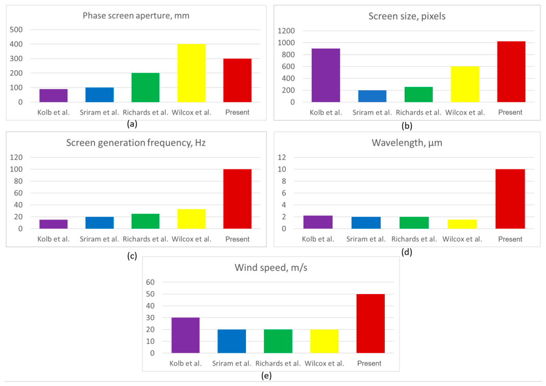
We compared the developed tool with respect to the existing analogues. A detailed analysis and comparison are contained in the Section 6 of the manuscript. Here, we briefly mention the main differences. The phase screen generator supports twice the aperture size (400 mm against 800 mm) and 1.5 times the phase screen generation size, in pixels (700 against 1024 pixels). It is also three times faster in phase screen generation compared to the fastest existing simulator version (33 Hz against 100 Hz). Another feature is the wavelength range—up to 10 µm against up to 2.2 µm in the existing simulator. The developed simulator also supports a much wider wind velocity range—it is 1.5 times wider (30 m/s in the existing tools compared to 50 m/s in the developed tool).

The architecture incorporates several distinguishing features:

• Native adaptive optics integration. Accepts unique influence functions from various wavefront correctors, including SLM, micro electro–mechanical systems (MEMS), bimorph mirrors, and stacked-actuator mirrors for phase screen reconstruction;
• High-performance parallel computation. Utilizes modern multi-core CPU processing power through .NET Task Parallel Library (TPL) [54] to solve high-order phase screen generation;
• Near-linear computational and memory complexity O(N). Transforms sequential O(N × m²) processes into parallel ones, where N represents the number of Zernike modes [55,56] and m is the phase screen grid linear resolution;
• Accessible desktop application. User-friendly graphical user interface (GUI), offline operation capability, and comprehensive data export functionality, unlike command line-driven research tools;
• Comprehensive parameter control. Full customization of key statistical parameters: refractive index structure parameter $C_n^2$, Fried radius ($r_0$), wind velocity, and radiation wavelength.

1.3. Motivation and Scientific Relevance

Computational efficiency is essential for modern optical engineering and scientific research. In closed-loop adaptive optics systems, real-time performance determines stability and correction accuracy, with phase screen reconstruction speed often being the limiting factor. The near-linear speedup achieved by this simulator enables real-time reconstruction in operational systems.

High-precision optical system development requires understanding how manufacturing tolerances and alignment errors affect performance, typically assessed through Monte Carlo simulations requiring thousands of ray-trace runs with randomly generated Zernike polynomial wavefront errors. The efficiency of this tool makes such large-scale statistical studies practical. Beyond classical adaptive optics, rapid Zernike surface generation supports specialized fields including computational microscopy for point-spread function engineering, super-resolution imaging, extended depth-of-field applications, and ophthalmology for custom contact lens design, refractive surgery planning, and understanding human vision limits.

The manuscript is organized as follows. Section 2 presents the theoretical basis for phase screen simulation, reconstruction methodology, and error analysis using influence functions of wavefront correction devices. Section 3 describes the developed software tool and parameter ranges. Section 4 presents validation demonstrating high accuracy and reconstruction frequency. Section 5 discusses the results. Section 6 concludes with a discussion of findings.

2. Theory: Phase Screen Simulation

2.1. Algorithm of Phase Screens Simulation

As established in the literature [57], one of the most computationally efficient and physically intuitive approaches to model optical wave propagation through atmospheric turbulence is the thin phase screen model. In this framework, a propagating optical wave encounters a sequence of thin screens that introduce phase distortions, effectively emulating the cumulative effects of propagation through a continuous randomly inhomogeneous medium. Each thin phase screen captures the influence of large-scale turbulent inhomogeneities on the phase of the optical field, and under a wide range of conditions, this approximation reproduces turbulence-induced wavefront aberrations with satisfactory fidelity [58].

To implement a time-evolving series of such screens, we employed a spectral method based on the fast Fourier transform (FFT) of the Kolmogorov turbulence spectrum [59]. The phase screen at a subsequent time step t + Δt is generated as:

$$p\left(u,v,t+∆t\right)={\displaystyle \underset{-\infty }{\overset{\infty }{\iint }}}\sqrt{K(x,y)}·f(x,y,t+∆t)·e^{i·\sqrt{{x·u}^2+{y·v}^2}·V·∆t}dxdy,$$

(1)

where $p\left(u,v,t+∆t\right)$ denotes the phase screen in the spatial domain at coordinates (x,y), and (x,y) are coordinates in the spatial frequency domain. Parameter V represents the transverse wind velocity (in m/s), t is the time of the previous screen generation, Δt is the temporal interval between successive screens, and K(x,y) is the spatial power spectral density of phase fluctuations. This spectrum is given by [60]:

$$K\left(x,y\right)=0.023·{({\displaystyle \frac{2D}{r_0}})}^{{\displaystyle \frac{5}{3}}}·{(x^2+y^2)}^{-{\displaystyle \frac{11}{3}}},$$

(2)

where D is the telescope aperture diameter and $r_0$ is the Fried parameter. The complex function f(x,y,t) introduces temporal evolution and stochasticity, and is defined recursively as:

$$f\left(x,y,t+∆t\right)=p·f\left(x,y,t\right)+\sqrt{1-p^2}·e^{i·\phi (x,y,t)},$$

(3)

with p = exp(−Δt/τ), where τ is the atmospheric coherence time. The term φ(x,y,t) is a random phase uniformly distributed in [0, 2π], uncorrelated in space and time. At the initial time step (t = 0), the function is initialized as:

$$f\left(x,y,t=0\right)=e^{i·\phi (x,y,t=0)}.$$

(4)

Following generation, the phase screen is normalized to ensure consistency with the expected phase structure function. The normalization enforces:

$$DN=6.88·{({\displaystyle \frac{\sqrt{x^2+y^2}}{r_0}})}^{{\displaystyle \frac{5}{3}}}.$$

(5)

Once a phase screen is generated, it can be decomposed into Zernike polynomials for further analysis or comparison.

Zernike polynomials constitute an essential mathematical basis for representing functions defined over the unit disk. They are widely used in a diverse range of scientific and engineering disciplines, including adaptive optics for characterizing atmospheric distortions, ophthalmology for quantifying ocular aberrations, microscopy for instrument characterization and aberration correction, and optical metrology for surface profiling. Zernike polynomials are defined in the following way (Equation (6)):

$$Z_n^m\left(\rho ,\theta \right)=\left\{\begin{array}{c}{R}_n^m\left(\rho \right)·\cos \left(m\theta \right)form\ge 0\\ R_n^{\left|m\right|}\left(\rho \right)·\sin \left(\left|m\right|\theta \right)form<0\end{array},\right.$$

(6)

where $\rho \in [0,1]$, $\theta \in [0,2\pi ]$ and $R_n^m$ is the radial part of Zernike polynomial that can be defined as follows (Equation (7)):

$$R_n^{\left|m\right|}\left(\rho \right)={\displaystyle \sum _{s=0}^{(n-\left|m\right|)/2}}{\displaystyle \frac{{\left(-1\right)}^s\left(n-s\right)!}{s!·\left(\frac{n+\left|m\right|}{2}-s\right)!·\left(\frac{n-\left|m\right|}{2}-s\right)!}}{\rho }^{n-2s}.$$

(7)

This decomposition enables a quantitative assessment of the simulated wavefront, for instance, by computing the pointwise residual between the original and approximated phase maps.

As can be seen, the phase screen generation procedure contains many summation operators, particularly at the phase screen calculation step, at the Fourier transform step, and at the phase values calculation step. These calculation stages present a performance bottleneck, since all calculations are performed linearly. Parallelizing these calculations using the TPL library might significantly decrease the generation time.

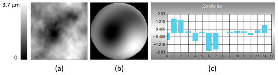
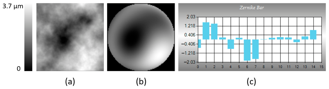
Using the phase screen simulation framework described above, we analyzed the statistical distribution of energy among Zernike modes in the simulated turbulent wavefronts. Based on an extensive ensemble of generated screens, the relative contribution of individual Zernike modes to the overall phase distortion is presented. Representative examples of a generated phase screen, its approximation with Zernike polynomials, along with the coefficient values, are shown in Figure 1.

2.2. Approximation/Reconstruction of Phase Screens Using Influence Functions

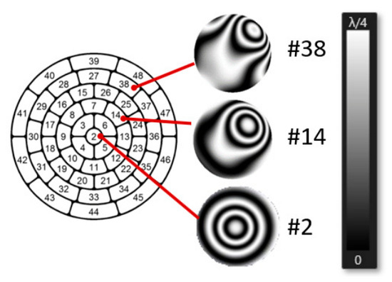
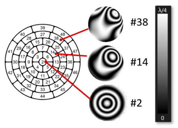
Following wavefront simulation, each generated phase screen was approximated using the influence functions of a piezoelectric mirror. An influence function characterizes the surface deformation induced by applying a unit signal to a single actuator of the active device (deformable mirror, spatial light modulator, MEMS, etc.); these functions (Figure 2) were experimentally measured using a Shack–Hartmann wavefront sensor. Interference patters peaks clearly coincide with the location of the active element of the piezoelectric mirror.

The reconstruction of the target phase screen using the mirror proceeded as follows:

The wavefront slopes were computed for each sub-aperture of the wavefront sensor based on the Zernike representation of the simulated phase screen. These slope values were converted into corresponding focal spot displacements on the sensor detector. Given the known relationship between actuator signals and focal spot displacements (i.e., the influence functions of the mirror), an overdetermined system of linear equations was formulated. The voltage vector minimizing the residual in the least squares sense was then obtained [61].

This procedure was applied independently to each simulated phase screen, yielding a set of control signal vectors. Each vector corresponds to a specific turbulent realization, and, when applied to the piezoelectric mirror, should produce a wavefront that closely matches the original simulated phase screen.

2.3. Reconstruction Error Analysis

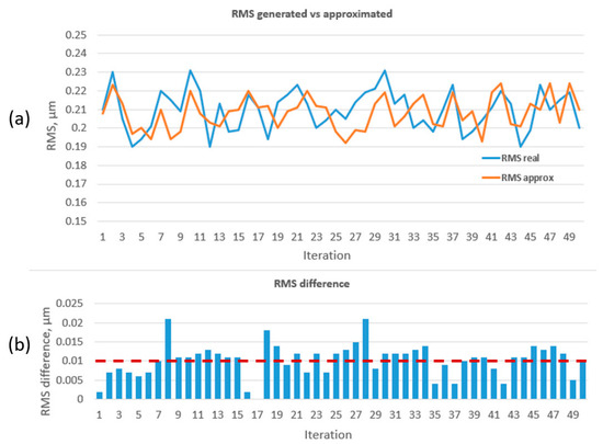
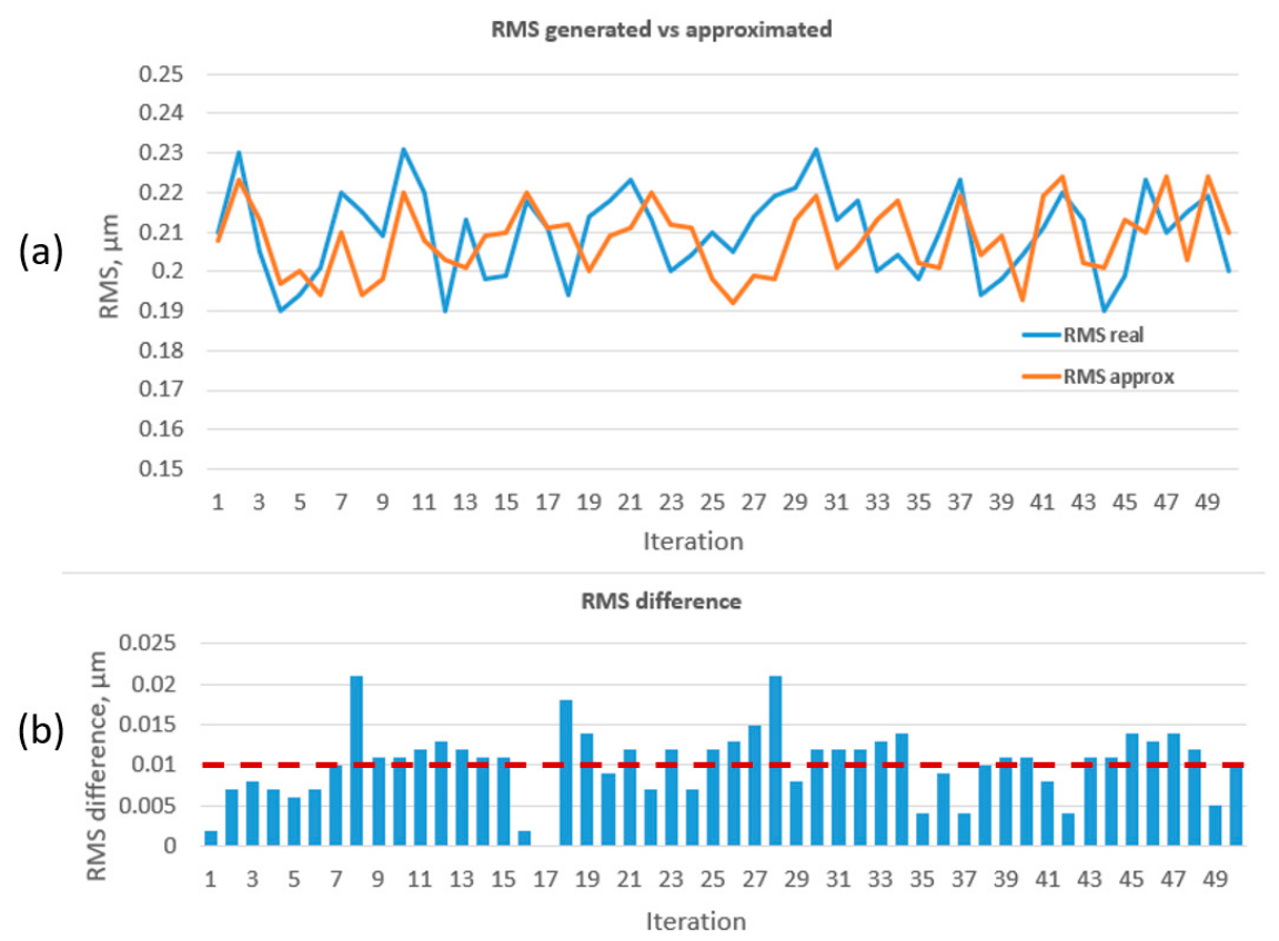
After simulating and reconstructing a set of phase screens, we performed the error analysis. Figure 3 presents the root mean square (RMS) error of a set of 50 generated and reconstructed phase screens along with the RMS difference bar chart.

RMS is calculated using the following equation:

$$RMS=\sqrt{{\displaystyle \frac{{\displaystyle {\sum }_{i=1}^N}{({\phi }_i-\widehat{\phi })}^2}{N}}},$$

(8)

where N—the number of phase screen points, ${\phi }_i$—phase value at ith point, $\widehat{\phi }$—average phase screen value.

It is clear from Figure 3 that the average RMS difference value ${RMS}_{diff}$ is about 0.01 µm. The average value of the RMS of generated phase screens ${RMS}_{gen}$ is 0.2 µm. The reconstruction error ${RMS}_{diff}/{RMS}_{gen}$ equals 5%.

3. Software: A Robust and Versatile Desktop Tool

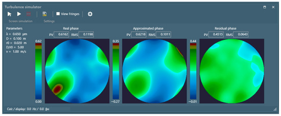
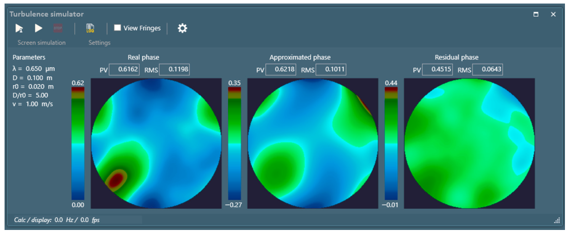
We designed the turbulence generator as a desktop tool in order to improve user experience. The graphical user interface is presented in Figure 4.

The layout is partitioned into two main parts. The toolbar contains the control buttons to run the phase screen generation procedure and to export the results into CSV file. The visualization canvas contains three sections to display phase/interference maps—generated one, reconstructed by the active device (piezoelectric mirror, spatial light modulator, etc.) one, and the point-to-point difference between the previous two maps. The section also contains the peak-to-valley values along with the RMS values.

The application enables the setup of parameters such as wavelength, telescope aperture diameter, Fried radius (or coherence radius that characterizes the resolution limit of the telescope; the greater the radius—the weaker the turbulence), and wind velocity. The type and range of parameters are presented in

Table 1. User-defined parameters of the turbulence simulator.

Parameter	Range
Wavelength, µm	0.1–10
Receiving aperture, m	0.01–10
Coherence radius, m	0.001–0.3
Wind speed, m/s	0.1–50
Zernike modes number	1–100
Calculation rate limit, Hz	1–1000
Phase screen resolution, px	32 × 32–1024 × 1024
Phase screen color palette	B&W, color
Measurement units	Microns, wavelengths

.

The application’s computational core centers on a phase calculation algorithm that derives the phase matrix from Zernike coefficients. To eliminate performance bottlenecks, computationally intensive loops are parallelized using the .NET Task Parallel Library (TPL).

The .NET platform was selected because: (1) it delivers high performance for CPU-bound numerical work; (2) it provides an integrated desktop development environment without needing separate GUI and backend components; (3) it offers robust built-in support for multithreading and parallel processing; and (4) it benefits from active development and a strong community. A key design goal was to avoid GPU dependence, ensuring that the tool remains performant and universally usable across diverse laboratory hardware.

4. Experiment: Phase Screens Reconstruction

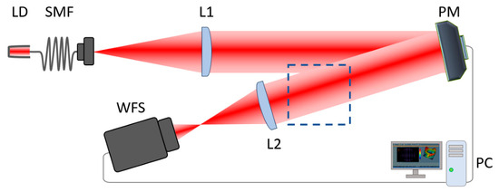
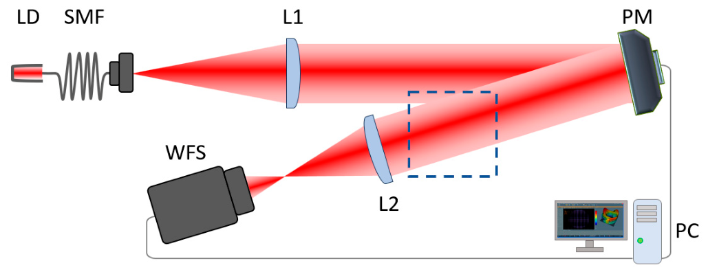
The principal scheme of the experimental setup that might be used for testing is depicted in Figure 5.

A fiber-coupled laser diode (LD) emitting at a wavelength of λ = 0.532 μm (FC/APC mount, CW, 5 mW, 4 μm fiber core, 0.9 mm diameter) is used as the optical source. The diode is pigtailed to a single-mode fiber (SMF). The output beam from the fiber is collimated by an achromatic lens (L1) with a focal length f = 400 mm, producing a beam with a diameter of 40 mm. The collimated beam propagates along the optical bench for a distance of 2 m before being reflected by a phase modulator (PM) [62,63]. The PM has a clear aperture of 50 mm and features 42 independent control elements. After reflection, the beam is directed into a receiving telescope composed of a second achromatic lens (L2) with a diameter of 50.8 mm and a focal length of f = 150 mm. This lens focuses the beam onto microlens array of the Shack–Hartmann wavefront sensor (WFS). The WFS output is digitized and interfaces with a control personal computer (PC) via a USB 3.0 connection. The acquired signal is processed in real time by our proprietary Turbulence Simulator software (version 1.0). The software computes a phase from the WFS and compares that phase with the numerically simulated phase screen, demonstrating the phase difference in real time [64,65,66].

In such a way, the user can see the phase screen that was numerically simulated, the phase screen that was experimentally reconstructed using the PM (the principle is described in Section 2.2), and the difference phase map with the reconstruction error.

5. Results

The primary parameter characterizing the intensity of atmospheric turbulence is the refractive index structure parameter $C_n^2$ [67]; specifically, a larger $C_n^2$ value indicates stronger turbulence. This parameter can range from ${10}^{-17} {\mathrm{m}}^{-{\displaystyle \frac{2}{3}}}$ for weak turbulence to ${10}^{-12} {\mathrm{m}}^{-{\displaystyle \frac{2}{3}}}$ for very strong atmospheric turbulence [68]. For instance, in Hefei, China, $C_n^2$ has been observed to vary between $6.69\times {10}^{-16}{\mathrm{m}}^{-{\displaystyle \frac{2}{3}}}$ and $9.87\times {10}^{-14}{\mathrm{m}}^{-{\displaystyle \frac{2}{3}}}$ during summer measurements along a horizontal atmospheric path of 1 km [69]. In maritime conditions, $C_n^2$ is approximately ${10}^{-15} {\mathrm{m}}^{-{\displaystyle \frac{2}{3}}}$ for a 10 km path with a coherence radius $r_0$ of $3.8\mathrm{c}\mathrm{m}$ at a laser wavelength $\lambda =0.85\mathsf{\mu }\mathrm{m}$ [70].

For ground-to-space communications between the International Space Station and the Optical Communications Telescope Laboratory (OCTL) in Wrightwood, California, a coherence radius of $r_0=4.5\mathrm{c}\mathrm{m}$ was experimentally determined for a 1200 km path at a zenith angle 75° with input telescope apertures ranging from $10\mathrm{c}\mathrm{m}$ to $100\mathrm{c}\mathrm{m}$ [71]. In terrestrial atmospheric turbulence, $C_n^2$ is approximately ${10}^{-12} {\mathrm{m}}^{-{\displaystyle \frac{2}{3}}}$ for a 1 km path under conditions where the wind velocity is 10 m/s and the telescope aperture is 20 cm [72,73]. In desert environments, $C_n^2$ measures around ${10}^{-13.2} {\mathrm{m}}^{-{\displaystyle \frac{2}{3}}}$ (with an average wind velocity of 6 m/s) along a 1.2 km path at Edward Air Force Base in the Mojave Desert, CA, USA [74]. The presented parameters are summarized in

Table 2. Turbulence parameters.

	Hefei, China	Maritime Conditions	Terrestrial Atmospheric Turbulence Conditions	Desert Environments
$C_n^2$	$6.69\times {10}^{-16} {\mathrm{m}}^{-{\displaystyle \frac{2}{3}}}$–$9.87\times {10}^{-14} {\mathrm{m}}^{-{\displaystyle \frac{2}{3}}}$	${10}^{-15}{\mathrm{m}}^{-{\displaystyle \frac{2}{3}}}$	${10}^{-12} {\mathrm{m}}^{-{\displaystyle \frac{2}{3}}}$	${10}^{-13.2} {\mathrm{m}}^{-{\displaystyle \frac{2}{3}}}$
Path	1 km	10 km	1 km	1.2 km
$r_0$	$3.8\mathrm{c}\mathrm{m}$	—	—	—

.

For test purposes, we used the following input parameters: wavelength 0.532 μm, aperture diameter 20 cm, Fried radius 1 cm, and wind velocity 6 m/s. Consequently, $C_n^2$ [67,68,69,70,71,72,73,74] varies approximately from $3.6\times {10}^{-14} {\mathrm{m}}^{-{\displaystyle \frac{2}{3}}}$ to $2.2\times {10}^{-13} {\mathrm{m}}^{-{\displaystyle \frac{2}{3}}}$ for path lengths ranging from 500 m to 3 km. We have tested the simulator on different parameter sets and selected the above set for demonstration purposes, as it corresponds to the average turbulence conditions.

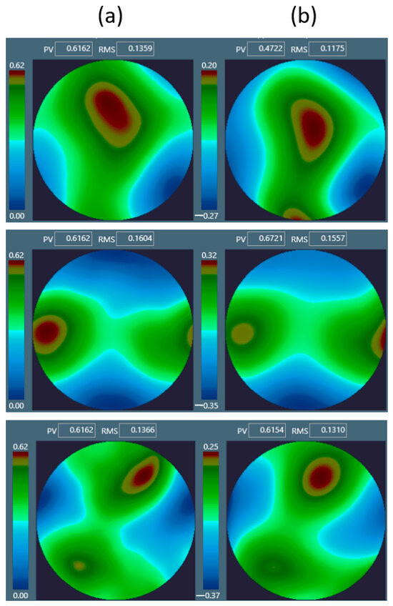
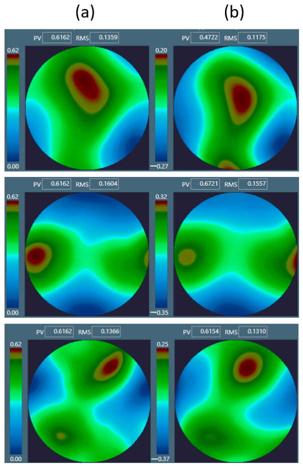
Figure 6 demonstrates, as an example, three sets of phase screens generated (numerically simulated) and reconstructed by the PM using the setup depicted in Figure 5.

Table 3. Zernike coefficients for the generated, approximated, and reconstructed phase screens.

Zernike Coefficients	Generated, µm	Approximated, µm	Reconstructed, µm
X-tilt	0.276826	0.271	0.268
Y-tilt	−0.00113	−0.0012	−0.0013
Focus	−1.31 × 10−5	0	0
Astig. vert.	0.104482	0.111	0.12
Astig. obl.	0.061853	0.062	0.0625
Coma horiz.	−0.1854	−0.187	−0.189
Coma vert.	0.000307	0.00031	0.00034
Spherical	0.020033	0.021	0.0213
Trefoil obl.	−0.16792	−0.168	−0.169
Trefoil vert.	0.014975	0.015	0.0155
Astig. vert. 2nd	−0.04535	−0.046	−0.0464
Astig. obl. 2nd	−0.06027	−0.061	−0.062
Coma horiz. 2nd	0.031487	0.032	0.033
Coma vert 2nd	−0.00446	−0.0045	−0.0046
Spherical 2nd	−0.00321	−0.0031	−0.0032
Tetrafoil vert.	−0.03873	−0.0375	−0.037
Tetrafoil obl.	−0.00378	−0.0038	−0.00381
Trefoil obl. 2nd	0.04106	0.042	0.043
Trefoil vert. 2nd	−0.01246	−0.013	−0.0132
Astig. vert. 3rd	0.012862	0.013	0.0131
Astig. obl. 3rd	0.024773	0.025	0.026
Coma horiz. 3rd	−0.00293	−0.003	−0.0031
Coma vert. 3rd	0.006868	0.0069	0.007
Spherical 3rd	−0.00108	−0.0012	−0.0013

contains the Zernike coefficients for the generated, approximated (using influence functions) and experimentally reconstructed phase screens.

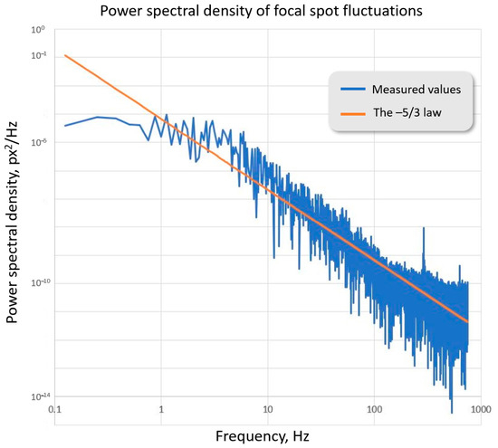
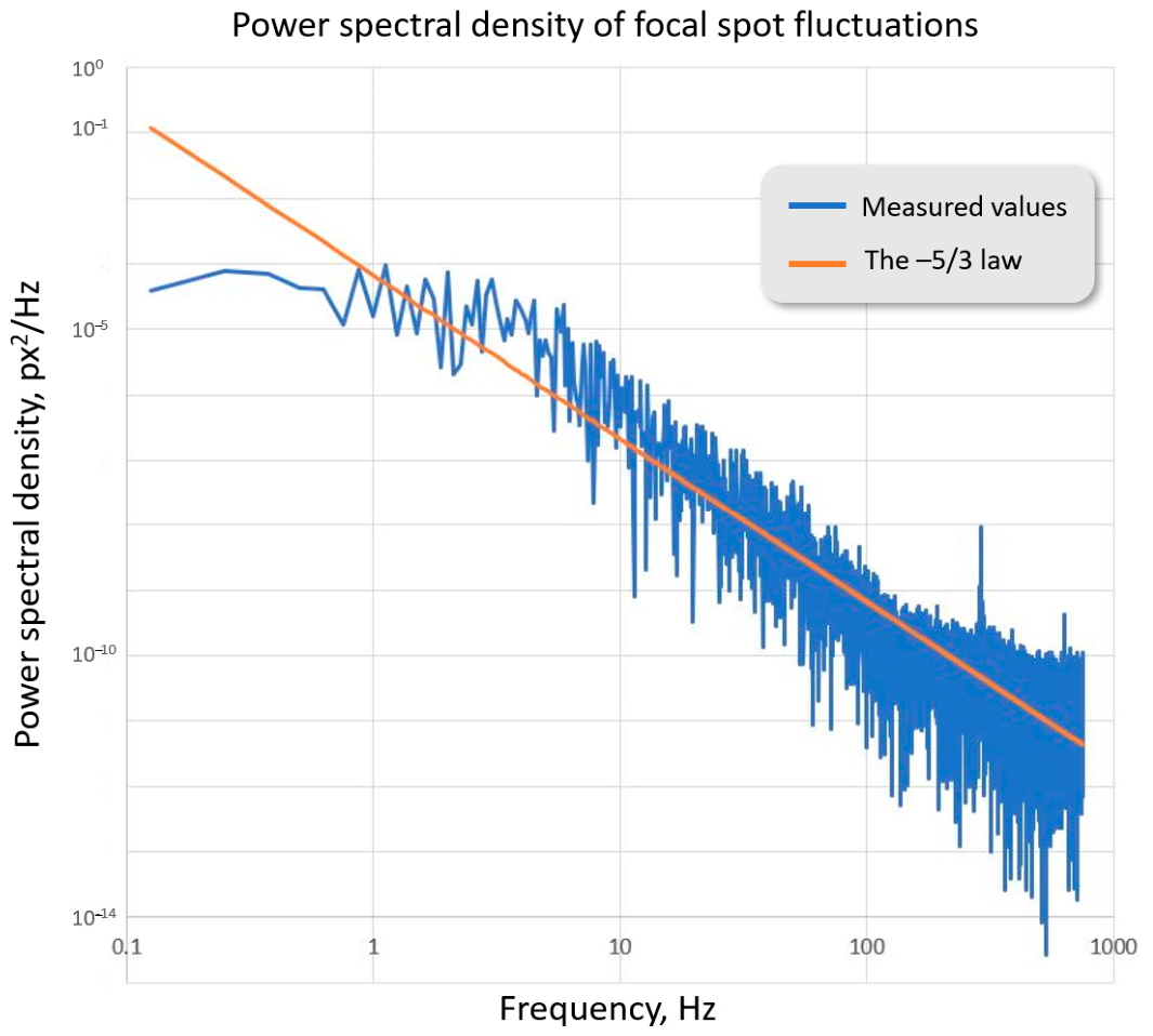
In order to be sure that the generated phase screen sequence coincides with the statistics of the Kolmogorov turbulent fluctuations, we calculated the 2D Fourier transform. The chart in Figure 7 demonstrates the power spectral density, where X axis is the frequency in log scale and Y axis is the power spectral density in log scale. Power spectral density is the function that describes the signal power distribution per unit frequency interval. We measured the jitter of a single focal spot on a Shack–Hartmann sensor in order to calculate the power spectral density. The orange line corresponds to the −5/3 law.

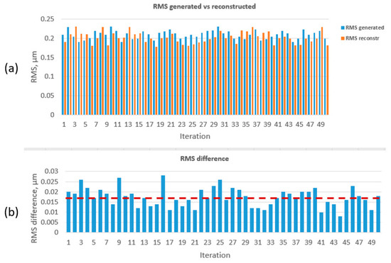
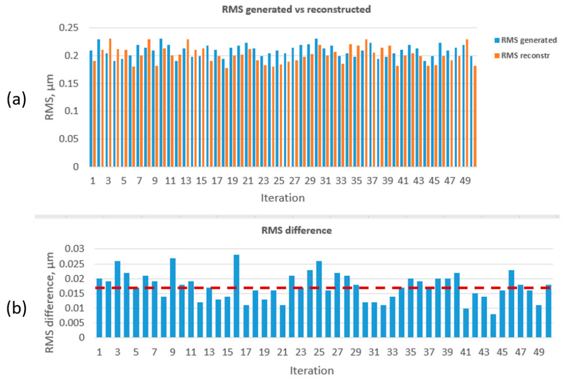
It can clearly be seen that the phase fluctuations of the generated phase screen lie within the Kolmogorov statistics. Figure 8 shows the bar diagram with the RMS values of the generated and reconstructed phase screens. The RMS values are calculated according to Equation (8).

The average RMS difference value ${RMS}_{diff-2}$ is approximately 0.017 µm. The average value of the RMS of generated phase screens ${RMS}_{gen}$ is 0.2 µm. The reconstruction error ${RMS}_{diff-2}/{RMS}_{gen}$ equals ~8%.

6. Discussion

Finally, we compared the developed tool with the existing solutions publicly available in the literature to date. The simulator created by Kolb et al. [49] allowed for the wavelength range to be set from 0.55 to 2.2 µm, a wind speed of 7, 13, and 30 m/s, with a phase screen size of 900 × 900. The developed simulator has a wider range, i.e., a wavelength up to 10 µm, a wind speed in the range of 1 to 50 m/s, and a path length of up to 20 km.

Sriram et al. [50] developed a phase screen generator that simulates a phase screen of 200 × 200 pixels in 20 ms, while the speedup due to using GPU is less than 20 times faster. Our developed simulator requires 16 ms to generate a phase screen of the same size; the speedup due to the parallel computation is 30 times faster.

Richards et al. [52] demonstrated an RMS error of more than 12% and a phase screen size that varied from 32 × 32 up to 256 × 256 pixels; the use of a GPU significantly increased the calculation time by up to 75 times. At the same time, the developed simulator achieved an 8% value for the RMS, enabled phase screens to be simulated by up to 1024 × 1024 pixels, and decreased the calculation time by 30 times compared to the single-core version.

Wilcox et al. [75] demonstrated a rather similar testbed for phase screen simulation using SLM, but with less functionality and variables range compared to the developed tool. The supported screen aperture was less than 400 mm; the screen size was less than 600 × 600 pixel. The screen generation frequency is rather low—about 30 Hz, which seems to be achieved by leveraging GPU, allowing for a speedup that is 30 times faster.

Table 4. Comparison of different turbulence simulator parameters.

Parameter	Kolb et al. [49]	Sriram et al. [50]	Richards et al. [52]	Wilcox et al. [75]	Present
Phase screen aperture, mm	90	100	200	≤400	10–800
Screen size, pixels	900 × 900	200 × 200	32 × 32–256 × 256	≤600 × 600	32 × 32–1024 × 1024
Screen generation frequency	15	20	25	≤33	100
GPU/Parallel-to-CPU speedup (Hz), times	—	≤20	4–75	30	30
Wavelength, µm	0.55–2.2	1–2	0.5–2	1–1.5	0.1–10
Wind speed, m/s	7, 13, 30	5–20	5–20	5–20	1–50
Framework	—	Matlab	Python	—	.NET

contains the abovementioned parameters.

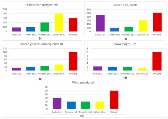
Figure 9 demonstrates the advantages of the developed simulator on various parameters, e.g., phase screen aperture, wavelength range, generation frequency, and wind speed range.

While the developed turbulence simulator outperforms most of the existing solutions on majority of parameters, it has drawbacks and disadvantages. First, the developed simulator cannot compete with simulators that leverage the GPU acceleration. The speed improvement of the solutions that use the GPU acceleration is much greater compared to the solutions that use CPU only. Another limitation is that the frequency of phase screen generation is basically calculated for a screen size of 256 × 256 pixels. The increase in resolution significantly decreases the generation frequency. This issue can be resolved either by using the parallelism on CPU or GPU. Our simulator is currently developed as a standalone application and thus cannot be integrated in mathematical packages such as Matlab and Mathworks. Such an integration might be useful, especially for educational purposes. We plan to solve the mentioned drawbacks in the next releases of the developed simulator.

7. Conclusions

In this research, we developed and investigated a software simulator and an experimental setup for reconstructing phase screens. The software–hardware system generated phase screens following Kolmogorov turbulence statistics, incorporating parameters for wind velocity and the D/r₀ ratio. Phase screens were produced at a rate of 100 Hz, which allowed for analysis of the beam behavior under even very strong atmospheric turbulence conditions, with an average approximation error of 0.01 µm (less than 5%). Compared to the fastest existing simulator, the developed phase screen generator offers twice the aperture size (800 mm vs. 400 mm) and 1.5 times the phase screen resolution in pixels (1024 vs. 700). It is also three times faster at generating phase screens, operating at 100 Hz rather than 33 Hz. Additionally, the new simulator supports a much broader wavelength range—up to 10 µm versus the existing 2.2 µm—and features a 1.5 times wider wind velocity range (50 m/s compared to 30 m/s). In experimental validation, the average reconstruction error was 0.017 µm, corresponding to approximately 8%. The developed tool can be used for performance analysis of wireless links due to its ability to estimate BER and quantum efficiency using the wavefront RMS.

The developed simulator might be used for both education purposes and preliminary laboratory tests. In the near future, we plan to release the second version of the simulator, providing even more interoperability with adaptive optics devices of different types and make the demonstration version of the simulator available online.

References

- Tatarsky, V.I. Waves Propagation in Turbulent Atmosphere; Nauka: Moscow, Russia, 1967. [Google Scholar]
- Andrews, L.C.; Phillips, R.L. Laser Beam Propagation Through Random Media, 2nd ed.; SPIE Press: Bellingham, WA, USA, 2005. [Google Scholar]
- Huang, Q.; Liu, D.; Chen, Y.; Wang, Y.; Tan, J.; Chen, W.; Liu, J.; Zhu, N. Secure free-space optical communication system based on data fragmentation multipath transmission technology. Opt. Express 2018, 26, 13536–13542. [Google Scholar] [CrossRef] [Scilit] [PubMed]
- Vorontsov, M.; Weyrauch, T.; Carhart, G. Lasers, Sources and Related Photonic Devices; OSA Technical Digest Series (CD); Optica Publishing Group Publisher: San Diego, CA, USA, 2010; p. LSMA1. [Google Scholar] [CrossRef] [Scilit]
- Khmelevtsov, S.S. Propagation of Laser Radiation in a Turbulent Atmosphere. Appl. Opt. 1973, 12, 2421–2433. [Google Scholar] [CrossRef] [Scilit]
- Nafria, V.; Han, X.; Djordjevic, I. Improving free-space optical communication with adaptive optics for higher order modulation. In Proceedings of the Optics and Photonics for Information Processing XIV, Online, 24 August–4 September 2020. [Google Scholar] [CrossRef] [Scilit]
- Mao, Y.; Cao, I.; Wang, Z.; Ma, X.; Gu, H.; Liu, W. Performance analysis of free space optical communications with FOA-WFS. Opt. Express 2024, 32, 28937–28952. [Google Scholar] [CrossRef] [Scilit]
- Weyrauch, T.; Vorontsov, M. Free-space laser communications with adaptive optics: Atmospheric compensation experiments. J. Opt. Fiber Comm. Rep. 2004, 1, 355–379. [Google Scholar] [CrossRef] [Scilit]
- Lema, G. Free space optics communication system design using iterative optimization. J. Opt. Commun. 2020, 44, 000010151520200007. [Google Scholar] [CrossRef] [Scilit]
- Zhang, Y.; Wang, Y.; Deng, Y.; Du, A.; Liu, J. Design of a Free Space Optical Communication System for an Unmanned Aerial Vehicle Command and Control Link. Photonics 2021, 8, 163. [Google Scholar] [CrossRef] [Scilit]
- Majumdar, A. Fundamentals of Free-Space Optical (FSO) Communication System. In Advanced Free Space Optics (FSO); Series in Optical Sciences; Springer: New York, NY, USA, 2015; Volume 186. [Google Scholar]
- Lu, M.; Bagheri, M.; James, A.P.; Phung, T. Wireless Charging Techniques for UAVs: A Review, Reconceptualization, and Extension. IEEE Access 2018, 6, 29865–29884. [Google Scholar] [CrossRef] [Scilit]
- Lukin, V.P.; Bol’basova, L.A.; Nosov, V.V. Comparison of Kolmogorov’s and coherent turbulence. Appl. Opt. 2014, 53, B231–B236. [Google Scholar] [CrossRef] [Scilit] [PubMed]
- Qin, S.; Liao, S. Clean numerical simulation of three-dimensional turbulent Kolmogorov flow. Phys. Fluids 2025, 37, 105160. [Google Scholar] [CrossRef] [Scilit]
- Guzev, M.; Doludenko, A.; Ermakov, A.; Posudnevskaya, A.; Fortova, S. Direct Numerical Simulation and Rank Analysis of Two-Dimensional Kolmogorov-type Vortex Flows. Supercomput. Front. Innov. 2025, 12, 43–59. [Google Scholar] [CrossRef] [Scilit]
- Chittoor, P.K.; Chokkalingam, B.; Mihet-Popa, L. A Review on UAV Wireless Charging: Fundamentals, Applications, Charging Techniques and Standards. IEEE Access 2021, 9, 69235–69266. [Google Scholar] [CrossRef] [Scilit]
- Wang, C.; Ma, Z. Design of wireless power transfer device for UAV. In Proceedings of the 2016 IEEE International Conference on Mechatronics and Automation, Harbin, China, 7–10 August 2016; pp. 2449–2454. [Google Scholar] [CrossRef] [Scilit]
- Geoffrey, A.; Landis, H. Laser beamed power—Satellite demonstration applications. In Proceedings of the 43rd International Astronautical Congress, Washington, DC, USA, 28 August–5 September 1992. [Google Scholar]
- Wang, R.; Wang, Y.; Jin, C.; Yin, X.; Wang, S.; Yang, C.; Cao, Z.; Mu, Q.; Gao, S.; Xuan, L. Demonstration of horizontal free-space laser communication with the effect of the bandwidth of adaptive optics system. Opt. Commun. 2018, 431, 167–173. [Google Scholar] [CrossRef] [Scilit]
- Toporovsky, V.; Galaktionov, I. Modal wavefront reconstruction of fixed aberrations for piezoelectric deformable mirrors. Lect. Notes Electr. Eng. 2026, 1521, 286–298. [Google Scholar] [CrossRef] [Scilit]
- Galaktionov, I.; Toporovsky, V. Gradient descent algorithm for automatic optimization of a laser beam cross-section in free-space optical communication applications. Lect. Notes Electr. Eng. 2026, 1521, 231–240. [Google Scholar] [CrossRef] [Scilit]
- Bennet, F.; Conan, R.; D’Orgeville, C.; Dawson, M.; Paulin, N.; Price, I.; Rigaut, F.; Ritchie, I.; Smith, C.; Uhlendorf, K. Adaptive optics for laser space debris removal. In Proceedings of the Adaptive Optics Systems III, Amsterdam, The Netherlands, 1–6 July 2012. [Google Scholar]
- Phipps, C.R.; Baker, K.L.; Libby, S.B.; Liedahl, D.A.; Olivier, S.S.; Pleasance, L.D.; Rubenchik, A.; Trebes, J.E.; George, E.V.; Marcovici, B.; et al. Removing orbital debris with lasers. Adv. Space Res. 2012, 49, 1283–1300. [Google Scholar] [CrossRef] [Scilit]
- Shen, S.; Jin, X.; Hao, C. Cleaning space debris with a space-based laser system. Chin. J. Aeronaut. 2014, 27, 805–811. [Google Scholar] [CrossRef] [Scilit]
- Galaktionov, I.; Toporovsky, V. A Multi-Deformable-Mirror 500 Hz Adaptive Optical System for Atmospheric Turbulence Simulation, Real-Time Reconstruction, and Wavefront Correction Using Bimorph and Tip-Tilt Correctors. Photonics 2025, 12, 592. [Google Scholar] [CrossRef] [Scilit]
- Barros, R.; Keary, S. Experimental setup for investigation of laser beam propagation along horizontal urban path. Proc. SPIE 2014, 9242, 396–404. [Google Scholar] [CrossRef] [Scilit]
- Mata-Calvo, R. Transmitter diversity verification on Artemis geostationary satellite. In Proceedings of the Free-Space Laser Communication and Atmospheric Propagation XXVI, San Francisco, CA, USA, 1–6 February 2014. [Google Scholar]
- Mosavi, N.; Marks, B.; Boone, B.; Menyuk, C. Optical beam spreading in the presence of both atmospheric turbulence and quartic aberration. In Proceedings of the Free-Space Laser Communication and Atmospheric Propagation XXVI, San Francisco, CA, USA, 1–6 February 2014. [Google Scholar]
- Murty, S.S.R. Laser beam propagation in atmospheric turbulence. Proc. Indian Acad. Sci. 1979, 2, 179–195. [Google Scholar] [CrossRef] [Scilit]
- Kwiecień, J. The effects of atmospheric turbulence on laser beam propagation in a closed space—An analytic and experimental approach. Opt. Commun. 2019, 433, 200–208. [Google Scholar] [CrossRef] [Scilit]
- Searles, S.; Hart, G.; Dowling, J.; Hanley, S. Laser beam propagation in turbulent conditions. Appl. Opt. 1991, 30, 401–406. [Google Scholar] [CrossRef] [Scilit] [PubMed]
- Gareth, D.; Naven, C. Experimental analysis of a laser beam propagating in angular turbulence. Open Phys. 2022, 20, 402–415. [Google Scholar] [CrossRef] [Scilit]
- Summerer, L.; Purcell, O. Concepts for wireless energy transmission via laser. J. Br. Interplanet. Soc. 2005, 58, 1–10. [Google Scholar]
- Fahey, T.; Islam, M.; Gardi, A.; Sabatini, R. Laser Beam Atmospheric Propagation Modelling for Aerospace LIDAR Applications. Atmosphere 2021, 12, 918. [Google Scholar] [CrossRef] [Scilit]
- Zohuri, B. Atmospheric Propagation of High-Energy Laser Beams. In Directed Energy Weapons; Springer: Cham, Switzerland, 2016. [Google Scholar]
- Shuto, Y. Effect of Water and Aerosols Absorption on Laser Beam Propagation in Moist Atmosphere at Eye-Safe Wavelength of 1.57 µm. J. Electr. Electron. Eng. 2023, 11, 15–22. [Google Scholar]
- Rosen, L.; Ipser, J. High Energy Laser Beam Scattering by Atmospheric Aerosol Aureoles. In Proceedings of the Nonlinear Optical Beam Manipulation and High Energy Beam Propagation Through the Atmosphere, Los Angeles, CA, USA, 5–20 January 1989. [Google Scholar]
- Oosterwijk, A.; Heikamp, S.; Manders-Groot, A.; Lex, A.; Eijk, J. Comparison of modelled atmospheric aerosol content and its influence on high-energy laser propagation. In Proceedings of the Laser Communication and Propagation Through the Atmosphere and Oceans VIII, San Diego, CA, USA, 11–15 August 2019. [Google Scholar]
- Galaktionov, I.; Toporovsky, V. A Multi-Stage Algorithm of Fringe Map Reconstruction for Fiber-End Surface Analysis and Non-Phase-Shifting Interferometry. Appl. Syst. Innov. 2026, 9, 31. [Google Scholar] [CrossRef] [Scilit]
- Soloviev, A.; Kotov, A.; Perevalov, S.; Esyunin, M.; Starodubtsev, M.; Alexandrov, A.G.; Galaktionov, I.V.; Samarkin, V.V.; Kudryashov, A.V.; Ginzburg, V.N. Adaptive system for wavefront correction of the PEARL laser facility. Quantum Electron. 2020, 50, 1115–1122. [Google Scholar] [CrossRef] [Scilit]
- Galaktionov, I.; Nikitin, A.; Sheldakova, J.; Toporovsky, V.; Kudryashov, A. Numerical Analysis of Wavefront Approximation Accuracy by Means of Zernike Polynomials for Optical Surface Flatness Measurements Using a Hartmannometer Device. Opt. Mem. Neural Netw. 2024, 33, S146–S157. [Google Scholar] [CrossRef] [Scilit]
- Buck, A.L. Effects of the Atmosphere on Laser Beam Propagation. Appl. Opt. 1967, 6, 703–708. [Google Scholar] [CrossRef] [Scilit] [PubMed]
- Galaktionov, I. ZernikeViewer: An Open-Source Framework for Fast Simulation and Real-Time Reconstruction of Phase, Fringe, and PSF Maps. Appl. Syst. Innov. 2026, 9, 51. [Google Scholar] [CrossRef] [Scilit]
- Galaktionov, I.; Toporovsky, V. Performance Analysis of an Optical System for FSO Communications Utilizing Combined Stochastic Gradient Descent Optimization Algorithm. Appl. Syst. Innov. 2025, 8, 143. [Google Scholar] [CrossRef] [Scilit]
- Khorin, P.; Khonina, S. Influence of 3D helical microstructure shape deviations on the properties of a vortex beam generated in the near diffraction zone. J. Opt. Technol. 2023, 90, 236–241. [Google Scholar] [CrossRef] [Scilit]
- Porfirev, A.; Khonina, S.; Khorin, P.; Ivliev, N. Polarization-sensitive direct laser patterning of azopolymer thin films with vortex beams. Opt. Lett. 2022, 47, 5080–5083. [Google Scholar] [CrossRef] [Scilit] [PubMed]
- Beason, M.K.; Hostutler, D.A.; Shock, S.; Kirby, D.; Schmucker, L.; Bates, E.M.; Miletich, T.; Budinski, V.; Pevec, S.; Njegovec, M.; et al. Laboratory Turbulence Generator for Evaluating Nodal Sensors. Proc. SPIE 2025, 13617, 51–61. [Google Scholar] [CrossRef] [Scilit]
- Mao, J.; Zhang, Y.; Li, J.; Gong, X.; Zhao, H.; Rao, Z. Novel Detection of Atmospheric Turbulence Profile Using Mie-Scattering Lidar Based on Non-Kolmogorov Turbulence Theory. Entropy 2023, 25, 477. [Google Scholar] [CrossRef] [Scilit] [PubMed]
- Kolb, J.; Oberti, S.; Marchetti, E.; Quirós-Pacheco, F. Full characterization of the turbulence generator MAPS for MCAO. In Proceedings of the Astronomical Telescopes + Instrumentation, Orlando, FL, USA, 27 June 2006; Volume 6272. [Google Scholar] [CrossRef] [Scilit]
- Sriram, V.; Kearney, D. An Ultra Fast Kolmogorov Phase Screen Generator Suitable For Parallel Implementation. Opt. Express 2007, 15, 13709. [Google Scholar] [CrossRef] [Scilit] [PubMed]
- Rinker, J. PyConTurb: An open-source constrained turbulence generator. J. Phys. Conf. Ser. 2018, 1037, 062032. [Google Scholar] [CrossRef] [Scilit]
- Richards, A.; Sutherland, J.; Saad, T. A Fast Turbulence Generator using Graphics Processing Units. In Proceedings of the 2018 Fluid Dynamics Conference, Atlanta, GA, USA, 25–29 June 2018. [Google Scholar] [CrossRef] [Scilit]
- Wilcox, C.; Martinez, T.; Santiago, F.; Andrews, J.R.; Restaino, S.R.; Teare, S.W.; Payne, D. Adaptive Optical System Atmospheric Turbulence Generator Testbed. Available online: https://www.researchgate.net/publication/242537340_Adaptive_Optical_System_Atmospheric_Turbulence_Generator_Testbed (accessed on 1 May 2026).
- Luo, Z.; Zheng, Q.; Hei, X.; Giacaman, N. Parallel Programming Based on Microsoft.NET TPL. In Proceedings of the 2nd International Conference on Computer Science and Electronics Engineering (ICCSEE 2013), Dubai, United Arab Emirates, 24–25 March 2013. [Google Scholar] [CrossRef] [Scilit]
- Dzyuba, A.P.; Khorin, P.A.; Serafimovich, P.G.; Khonina, S.N. Wavefront Aberrations Recognition Study Based on Multi-Channel Spatial Filter Matched with Basis Zernike Functions and Convolutional Neural Network with Xception Architecture. Opt. Mem. Neural Netw. 2024, 33, S53–S64. [Google Scholar] [CrossRef] [Scilit]
- Khorin, P.; Volotovskiy, S. Analysis of the threshold sensitivity of a wavefront aberration sensor based on a multi-channel diffraction optical element. Proc. SPIE 2021, 11793, 62–73. [Google Scholar] [CrossRef] [Scilit]
- Kandidov, V.; Shlenov, A. Atmospheric Turbulence Simulation. Grid Representation; Technical Summary; International Laser Center: Moscow, Russia, 1995. [Google Scholar]
- Vorontsov, M.; Shmalhausen, V. Principles of Adaptive Optics; Nauka: Moscow, Russia, 1985. [Google Scholar]
- Dudorov, V.; Kolosov, V.; Filimonov, G. Algorithm for formation of an infinite random turbulent screen. In Proceedings of the Twelfth Joint International Symposium on Atmospheric and Ocean Optics/Atmospheric Physics, Tomsk, Russia, 27–30 June 2005. [Google Scholar]
- Lane, R.G.; Glindemann, A.; Dainty, J.C. Simulation of a Kolmogorov phase screen. Waves Random Media 1992, 2, 209–224. [Google Scholar] [CrossRef] [Scilit]
- Li, J.; Li, W.; Huang, R. An efficient method for solving a matrix least squares problem over a matrix inequality constraint. Comput. Optim. Appl. 2016, 63, 393–423. [Google Scholar] [CrossRef] [Scilit]
- Skvortsov, A.A.; Zuev, S.M.; Koryachko, M.V.; Voloshinov, E.B. Specific features of motion of molten zones in the field of silicon structural inhomogeneity. Tech. Phys. Lett. 2017, 43, 705–707. [Google Scholar] [CrossRef] [Scilit]
- Koryachko, M.V.; Pshonkin, D.E.; Skvortsov, A.A. Features of melt droplet formation during electrical destruction aluminum films on the semiconductor surface. Defect Diffus. Forum 2021, 410, 737–741. [Google Scholar] [CrossRef] [Scilit]
- Skvortsov, A.A.; Koryachko, M.V.; Zuev, S.M.; Demchenkova, A.A. Melt drops movement over semiconductor surfaces controlled by electric field. Period. Tche Quim. 2019, 16, 681–687. [Google Scholar] [CrossRef] [Scilit]
- Soloviev, A.A.; Kotov, A.V.; Martyanov, M.A.; Perevalov, S.E.; Zemskov, R.S.; Starodubtsev, M.; Aleksandrov, A.; Galaktionov, I.; Samarkin, V.; Kudryashov, A.; et al. Improving focusability of post-compressed PW laser pulses using a deformable mirror. Opt. Express 2022, 30, 40584–40591. [Google Scholar] [CrossRef] [Scilit] [PubMed]
- Samarkin, V.; Alexandrov, A.; Galaktionov, I.; Kudryashov, A.; Nikitin, A.; Rukosuev, A.; Toporovsky, V.; Sheldakova, J. Large-aperture adaptive optical system for correcting wavefront distortions of a petawatt Ti: Sapphire laser beam. Quantum Electron. 2022, 52, 187–194. [Google Scholar] [CrossRef] [Scilit]
- Burger, L.; Litvin, I.; Forbes, A. Simulating atmospheric turbulence using a phase-only spatial light modulator. S. Afr. J. Sci. 2008, 104, 129–137. [Google Scholar]
- Laslandes, M.; Patterson, K.; Pellegrino, S. Optimized actuators for ultrathin deformable primary mirrors. Appl. Opt. 2015, 54, 4937–4952. [Google Scholar] [CrossRef] [Scilit] [PubMed]
- Liu, D.; Wang, Z.; Liu, J.; Tan, J.; Yu, L.; Mei, H.; Zhou, Y.; Zhu, N. Performance analysis of 1-km free-space optical communication system over real atmospheric turbulence channels. Opt. Eng. 2017, 56, 106111. [Google Scholar] [CrossRef] [Scilit]
- Li, M.; Cvijetic, M. Coherent free space optics communications over the maritime atmosphere with use of adaptive optics for beam wavefront correction. Appl. Opt. 2015, 54, 1453–1462. [Google Scholar] [CrossRef] [Scilit] [PubMed]
- Wright, M.W.; Morris, J.F.; Kovalik, J.M.; Andrews, K.S.; Abrahamson, M.J.; Biswas, A. Adaptive optics correction into single mode fiber for a low Earth orbiting space to ground optical communication link using the OPALS downlink. Opt. Express 2015, 23, 33705–33712. [Google Scholar] [CrossRef] [Scilit] [PubMed]
- Thompson, C.A.; Kartz, M.W.; Flath, L.M.; Wilks, S.C.; Young, R.A.; Johnson, G.W.; Ruggiero, A.J. Free space optical communications utilizing MEMS adaptive optics correction. In Proceedings of the Free-Space Laser Communication and Laser Imaging II, Seattle, WA, USA, 7–11 July 2002. [Google Scholar]
- Cornelissen, S.; Hartzell, A.; Stewart, J.; Bifano, T.; Bierden, T. MEMS Deformable Mirrors for Astronomical Adaptive Optics. In Proceedings of the Adaptive Optics Systems II, San Diego, CA, USA, 27 June–2 July 2010. [Google Scholar]
- Majumdar, A.K.; Eaton, F.D.; Jensen, M.L.; Kyrazis, D.T.; Schumm, B.; Dierking, M.P.; Shoemake, M.A.; Dexheimer, D.; Ricklin, J.C. Atmospheric Turbulence Measurements over Desert site using groundbased instruments, kite/tethered-blimp platform and aircraft relevant to optical communications and imaging systems: Preliminary Results. In Proceedings of the Free-Space Laser Communications VI, San Diego, CA, USA, 13–17 August 2006. [Google Scholar]
- Wilcox, C.C.; Martinez, T.; Santiago, F.; Andrews, J.R.; Restaino, S.R.; Teare, S.W.; Payne, D.M. Atmospheric turbulence generator for adaptive optical systems testing. In Proceedings of the SPIE Optical Engineering + Applications, San Diego, CA, USA, 27 September 2007; Volume 6711. [Google Scholar] [CrossRef] [Scilit]
Disclaimer/Publisher’s Note: The statements, opinions and data contained in all publications are solely those of the individual author(s) and contributor(s) and not of MDPI and/or the editor(s). MDPI and/or the editor(s) disclaim responsibility for any injury to people or property resulting from any ideas, methods, instructions or products referred to in the content. |
© 2026 by the author. Licensee MDPI, Basel, Switzerland. This article is an open access article distributed under the terms and conditions of the Creative Commons Attribution (CC BY) license.