Article

Time-Varying Biological Time-Series Prediction and Pattern Recognition Using Koopman Theory and Large Language Models


by
Yujie You
1,
Yuzhu Ji
1,
Salavat Gumerovich Mudarisov
2,
Ilnur Rinatovich Miftakhov
2,
Feixiang Zhao
1,
Ming Xiao
3 and
Le Zhang
3,*
1
School of Computer Science and Engineering, Sichuan University of Science and Engineering, Yibin 644000, China
2
Department of Mechatronic Systems and Agricultural Machines, Bashkir State Agrarian University, 34, ul. 50-Letiya Oktyabrya, 450001 Ufa, Russia
3
College of Computer Science, Sichuan University, Chengdu 610065, China
*
Author to whom correspondence should be addressed.
Technologies 2026, 14(6), 321; https://doi.org/10.3390/technologies14060321
Submission received: 15 April 2026 / Revised: 21 May 2026 / Accepted: 22 May 2026 / Published: 25 May 2026

Abstract

Biologically related time-series data characterize the dynamic evolution of biological systems, including genetic inheritance, disease diagnosis, and the biological microenvironment. However, accurate prediction of these data remains challenging due to their pronounced time-varying, non-stationary, and noisy characteristics. Existing approaches often fail to capture latent shifts of biologically related time series, limiting both predictive performance and time-varying pattern recognition capability. Thus, in this study, we first propose a time-varying neural network (TVNN) model that combines frequency-domain information with Koopman theory. TVNN-model Koopman transition matrices are used to model global dynamics and local time-varying behaviors for pattern extraction. Secondly, a time-varying pattern recognition large language model (TVPRLLM) is introduced to recognize and classify the extracted time-varying patterns, enabling the identification of potential pattern categories. Thirdly, we have developed a biology-related time-series predictive platform that can offer visualization, data analysis, and predictive services. Experimental results demonstrate that the TVNN model outperforms existing mainstream methods in predicting biology-related time-varying time series, and that it achieves competitive forecasting performance, though its behavior depends strongly on the design of the frequency-domain decomposition. Additional robustness analyses reveal that the choice of Fourier masking strategy can materially affect both RMSE and long-horizon stability. We further show that Koopman-derived time-varying representations are highly discriminative for dynamic state recognition.

1. Introduction

Driven by the rapid development of high-throughput sequencing technologies [1], biology-related time-series data have seen substantial growth, spanning multi-omics molecular profiles, microbial environmental observations, and clinical monitoring records. Such heterogeneous data offer a dynamic and multidimensional view of biologically related systems across both temporal and spatial dimensions, thereby creating unprecedented opportunities for biomedical discovery, environmental microbiology research, and clinical decision making. In this context, biologically related time-series prediction uses past observations to predict future states. It not only aids in deciphering the regulatory dynamics of living systems and their interactions with the environment, but also contributes to precision medicine by supporting diagnosis, prognosis, and treatment planning.
Yet biologically related systems are not static entities; they are time-varying systems, with molecular activities, physiological processes, biochemical reactions, and environmental interactions evolving over time [2]. The temporal variability is reflected, including gene regulatory activity, protein modification, environmental interactions, and so on. As the intrinsic mechanisms of living systems and the extrinsic environments vary dynamically, biologically related time-series data often exhibit non-stationary behavior [2]. Figure 1 illustrates a Lorenz system [3] with different time-varying patterns, which is an idealized representation of chaotic gene regulatory dynamics. These temporal shifts may be driven by disease progression, treatment responses, or ecological perturbations, which in turn induce changes in covariate patterns across time steps. The changes in data distribution and statistical properties present substantial challenges to accurate, biologically related time-series prediction.
The Lorenz system is used to model chaotic gene regulatory networks in biologically related time-varying systems [3]. Red can be intuitively interpreted as an active dynamic regime, which may correspond to pronounced gene-expression fluctuations, black is conceptually compared to a transitional regime reflecting switching, and blue may represent a relatively stable or alternative oscillatory regime.
Early studies on biologically related time-series prediction mainly focused on time-domain analysis using classical statistical models [4,5], such as Autoregression (AR) [6] and Autoregressive Integrated Moving Average (ARIMA) [7]. However, these methods rely on the assumption of stationarity of biologically related systems. With the development of deep learning, the RevIN model has been proposed to restore the varying mean and variance [8]. It transforms the predictive task into modeling a relatively stationary sequence. Although such methods can increase predictive accuracy, they mainly focus on statistical components and remain limited in frequency structures, which makes them less suitable for time-varying biologically related systems.
As a novel perspective for biologically related time-series prediction, Koopman theory [9] can embed nonlinear dynamical systems into an infinite-dimensional linear space, where the evolution follows linear dynamics and preserves the nonlinear characteristics of the original system. Using the Koopman theory, Liu et al. [10] proposed a Koopa forecaster, which characterizes the temporal dynamics in non-stationary sequences. The experimental results indicate that Koopa can achieve high performance in influenza and climate prediction. Meanwhile, frequency-domain information can effectively separate periodic components from evolving components [11,12]. Such decomposition may help to reveal the time-varying characteristics of a biologically related system. Therefore, how to integrate frequency-domain information into Koopman theory to construct a unified neural modeling framework for time-varying, biologically related systems becomes our first scientific problem.
Although biologically related time-series prediction models can predict future states, it is hard to reveal the time-varying behaviors of biologically related systems. To attempt to solve this problem, Wang et al. [13] used Koopman theory to uncover hidden time-varying patterns in biologically related time-series data. Although their method captures the pattern features, it provides limited capability for recognizing biologically relevant time-varying patterns. The development of large language models (LLMs), such as GPT-4 [14] and Qwen2 [15], has created new opportunities to enhance the recognition of time-varying patterns due to their strong pattern recognition capabilities. Therefore, how to combine Koopman theory with LLMs to build a time-varying pattern recognition model and identify patterns encoded in the Koopman transition matrix becomes our second scientific problem.
To further support biologically related research practice, relevant methods are often transformed into platform-based tools to decrease usage barriers and increase their practical value [16,17]. For example, MathIOmica [18] enables in-depth analysis of multi-omics time-series data through multi-scale temporal trajectory modeling and supports the visualization of spatiotemporal correlations, while MOVIS [19] provides embedding and interactive visualization for multimodal biologically related time-series data. However, these platforms mainly focus on multi-omics data analysis and provide limited support for predictive tasks across broader types of biologically related time-series data. In addition, most existing predictive models are released as software packages [20], which often lack user-friendly interfaces and operational convenience. Therefore, how to build a biologically related time-series predictive platform with a friendly user experience becomes our third scientific problem.
To address the above three scientific problems, we propose a time-varying neural network (TVNN), which combines frequency-domain information with Koopman theory. The network effectively extracts non-stationary representations of biologically related time-series data and conducts nonlinear dynamic inference on time-varying biologically related systems, thereby realizing highly efficient prediction of their time-series data. Secondly, by incorporating a large language model fine-tuned collaboratively with LoRA, a time-varying pattern recognition large language model (TVPRLLM) is constructed to identify and classify the time-varying patterns of these biologically related systems. Finally, we developed a biologically related time-series prediction platform to provide users with efficient prediction services. Here, we carried out a comprehensive evaluation of our TVNN model on six biologically related time-series datasets and demonstrated that our proposed method outperforms existing mainstream methods in time-series prediction for time-varying biologically related systems.

2. Materials and Methods

2.1. Experimental Datasets

We evaluated the proposed model on six biologically related time-series datasets: Proteomics, Gene, Solar, EMG, Climate, and ILI. These datasets span multiple biologically related scales, including two simulated datasets, molecular expression and gene regulation, and four real datasets: physiological state monitoring, environmental drivers of biologically related activity, and population-level disease dynamics.
Proteomics: Proteomics exhibit a complex and dynamic time-varying behavior. The time-series data show a distinct oscillatory trend. To mimic the unstable oscillatory behavior observed in protein expression [21,22], we adopt the nonlinear pendulum system [23]:
d 2 θ d t 2 + g l s i n θ = 0 θ t 0 = θ 0
where l is the pendulum’s length, g is the gravitational acceleration, and θ 0 is the initial condition. A greater θ 0 implies stronger nonlinear interactions among proteins. To account for biologically related variability and measurement noise commonly encountered in real proteomic data [3], Gaussian white noise [24] is added:
x ~ i t = x i t + ε i ,   ε i ~ N ( 0 , σ 2 )
where x ~ i t represents the noisy ith-dimensional data at time step t . The noise term ε i follows a normal distribution ε i ~ N ( 0 , σ 2 ) , where σ indicates the noise intensity. In this experiment, we set θ 0 = 2.4 and σ = 0.1 to generate a sequence of 2000 steps, and project it into a 32-dimensional space through random orthogonal transformation [25].
Gene: Gene regulatory networks are highly nonlinear and chaotic systems that reflect the dynamic interplay of transcriptional regulation and feedback control [3]. To model these characteristics, we generate data using the Lorenz system [26]:
x t + 1 = x t + h η y t z t y t + 1 = z t + h x t ρ z t y t z t + 1 = z t + h ( x t y t β z t )
where η , ρ , and β are constants, and h controls the interaction strength. Greater h values correspond to stronger nonlinear coupling among genes.
Solar: The seasonal and time-varying differences in solar radiation directly affect biologically related growth and metabolism. The dataset [27] was collected from 137 photovoltaic power plants in Alabama at a 10 min sampling interval. Predicting solar radiation patterns aids in understanding ecosystem mechanisms and conserving biodiversity.
EMG: Muscle states during sustained contraction change dynamically over time. The EMG dataset [28] records EMG signals from subjects maintaining 20% of their maximum grip strength until muscle fatigue. Predicting the time-frequency domain features of these signals helps us reveal the physiological mechanisms underlying fatigue, providing a medical basis for muscle rehabilitation training.
Climate: Climate is a complex time-varying system that acts as a fundamental driver of ecological processes and biologically related dynamics. This dataset [29] records 21 meteorological indicators, including temperature and humidity, at 10 min intervals throughout the year 2020. Accurate climate prediction can help us quantify the effects of environmental change on biologically related systems and ecosystem resilience.
ILI: Influenza-like illness exhibits pronounced temporal variability driven by viral mutation, host immunity, and seasonal transmission patterns. This dataset [29] tracks the weekly number of patients with influenza-like illness recorded by the U.S. CDC from 2002 to 2021. Modeling its temporal evolution is valuable for outbreak prediction, epidemiological surveillance, and public health intervention planning.

2.2. Problem Setting

Let S t ( t ) H denote the underlying state of a biologically related system, where H is a finite-dimensional vector space, and let Z ( t ) R D denote its observed time-series measurement. For the observed biologically related time-series data Z = ( Z 1 , , Z t , Z M ) R D × M , D and M represent the variable dimension and the number of observed time-series steps, respectively. The biologically related system is described by
S t ( t ) t = A ( S t ( t ) )
Z t + 1 = B ( Z t )
where A is the governing equation of the system, and B characterizes the evolution of the observed data. Our first objective is to learn a mapping function F that predicts the future L steps from M historical observation. Formally, given observed biologically related time-series data Z , the goal is to estimate Z ^ p R D × L :
Z ^ p = ( Z ^ M + 1 p ,   Z ^ M + 2 p , . ,   Z ^ M + L p ) = F ( Z 1 ,   Z 2 , . , Z t , ,   Z M )
Our second objective is to learn another mapping function G that maps latent dynamic representations to predefined biologically related time-varying pattern labels. Specifically, the M historical observations are divided into S segments of equal length M / S . For a segment beginning at time step t , G takes ( Z t ,   Z t + 1 , , Z t + M / S 1 ) as input and outputs the latent state s t a t e t of the biologically related system:
s t a t e t = G ( Z t , Z t + 1 , , Z t + M / S 1 )

2.3. Time-Varying Neural Network

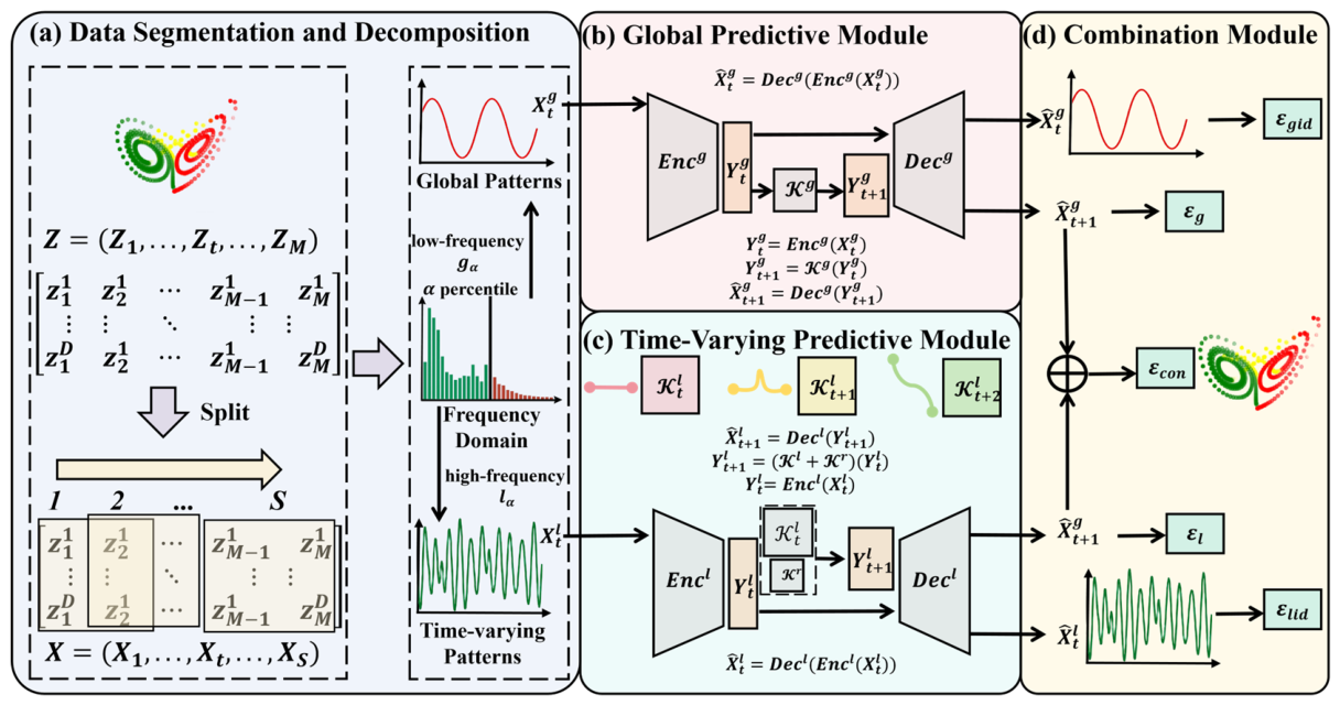
As illustrated in Figure 2, to accomplish the task objectives described in Section 2.1, we develop a time-varying neural network (TVNN) for biologically related time-series prediction to realize the mapping function F . This section is composed of four parts: data segmentation and decomposition, global prediction module, time-varying predictive module, and combination module.

2.3.1. Data Segmentation and Decomposition

Lin et al. [30] demonstrated that segment-wise iteration achieves better predictive performance than point-wise iteration for time-series prediction. Accordingly, given the observed biologically related time-series data Z = ( Z 1 ,   , Z t , Z M ) R D × M , where Z t = ( z 1 ,   . ,   z D ) R D , we divide the data into S segments of equal length M / S . The segmented sequence is denoted as X = ( X 1 ,   , X t , X s ) , where X t = ( Z ( t 1 ) M / S + 1 ,   Z ( t 1 ) M / S + 2 , . , Z t M / S ) R D × ( M / S ) .
For biologically related time-series data, low-frequency global patterns characterize the organism’s fundamental physiological states or long-term trends, whereas high-frequency time-varying patterns reflect transient physiological responses or stimulus-induced fluctuations. Motivated by Liu et al. [10], who verified the effectiveness of Fourier filter decomposition for time-series prediction, we employ Fourier filtering [11,12] to decompose each segment X t in the frequency domain. As a result, each segment is separated into low-frequency global patterns X t g and high-frequency time-varying patterns X t l , formulated as
X t g = F 1 ( g α ( F ( X t ) ) )
X t l = F 1 ( l α ( F ( X t ) ) )
X t = X t g + X t l
Specifically, a Fast Fourier Transform (FFT) is applied to each segment X t . Components with frequency below the α   p e r c e n t i l e are preserved as low-frequency global components, while those above the α   p e r c e n t i l e are regarded as high-frequency time-varying components. Here, g and l denote the global and time-varying filters, respectively; α is a hyperparameter; F denotes the Fourier Transform; and F 1 denotes the Inverse Fourier Transform.

2.3.2. Global Predictive Module

In biologically related systems, low-frequency global patterns characterize changes and responses that occur over relatively long-time scales and are associated with macroscopic processes. Reconstructing such patterns can help us reveal the intrinsic laws governing the long-term evolution of biologically related systems.
In this study, we employ an encoder–decoder architecture to project the observed data onto a high-dimensional measurement space. A linear Koopman operator is then applied to model the evolution of the global patterns and infer the trajectory of the low-frequency global dynamics:
X ^ t + 1 g = D e c g ( K g ( E n c g ( X t g ) ) )
where E n c g : R D × ( M / S ) R D × d denotes the projection encoder, K g : R D × d R D × d denotes the Koopman transition operator, and D e c g : R D × d R D × ( M / S ) denotes the projection decoder for the global patterns. Both E n c g and D e c g are implemented as feed-forward neural networks.

2.3.3. Time-Varying Predictive Module

High-frequency time-varying patterns characterize the changes and responses of biologically related systems over short time scales. These patterns involve microscopic and mesoscopic processes, such as individual physiological activities and interactions among organisms. Reconstructing high-frequency time-varying patterns helps us reveal the local temporal variation trends of biologically related systems over extended periods.
In this study, we employ an encoder, E n c l : R D × ( M / S ) R D × d , to project the observed data onto a high-dimensional measurement space, yielding Y t l . Here, E n c l is implemented as a feed-forward neural network.
Y t l = E n c l ( X t l )
Subsequently, for each high-dimensional representation Y t l , the time-varying predictive module employs the Dynamic Mode Decomposition (DMD) algorithm [31] to compute the Koopman operator K t l (Equation (13)). The operator K t l is then used to drive the evolution of high-frequency time-varying trajectories (Equation (14)).
K t l = Y t + 1 l Y t l +
Y ^ t + 1 l = K t l ( Y t l )
where Y t l + denotes the generalized inverse of Y t l , satisfying Y t l Y t l + = i d , where i d represents the identity matrix.
In addition, as residual errors are inevitable in reconstructing time-varying patterns, a learnable Koopman residual matrix K r is introduced to dynamically adjust and compensate for reconstruction errors (Equation (15)). This mechanism accounts for both system modeling errors and real-world disturbances:
Y ^ t + 1 r = K r ( Y t l )
Finally, the decoder D e c l : R D × d R D × ( M / S ) is used to map the high-dimensional representations back to the original measurement space, thereby reconstructing X ^ t l (Equation (16)). Meanwhile, to ensure that the decoder can also reconstruct the states evolved by the Koopman operator and thus improve the generalization ability of the predictive model, D e c l further projects the evolved representation Y ^ t + 1 l back to the measurement space to reconstruct X ^ t + 1 l (Equation (17)). Here, D e c l is also implemented as a feed-forward neural network.
X ^ t l = D e c l ( Y t l )
X ^ t + 1 l = D e c l ( Y ^ t + 1 l + Y ^ t + 1 r ) = D e c l ( ( K t l + K r ) E n c l ( X t l ) )

2.3.4. Combination Module

The final prediction is obtained by combining the outputs of the global predictive module and the time-varying predictive module. Specifically, the evolution of the observed data is expressed as
X ^ t + 1 = X ^ t + 1 g + X ^ t + 1 l
Following the segmentation scheme described in Section 2.3.1, the predictive estimate Z ^ p is rearranged into segmented form X ^ p =   ( X ^ S + 1 p , , X ^ S + t p , ,   X ^ S + L S / M p ) , where X ^ S + t p = ( Z ^ M + M t / S + 1 p , . , Z ^ M + M ( t + 1 ) / S p ) . Under this partitioning scheme, each segment predicted segment X ^ S + t p is computed as
X ^ S + t g = D e c g ( K g ( t ) ( E n c g ( X S g ) ) )
X ^ S + t l = D e c l ( ( K S 1 l + K r ) ( t ) ( E n c l ( X S l ) ) )
X ^ S + t p = X ^ S + t g + X ^ S + t l
Because the TVNN contains trainable encoders and decoders in both prediction modules, together with the global Koopman transition operator K g , the entire framework can be trained end-to-end. The training objective consists of five loss terms: global reconstruction loss ε g i d , global prediction loss ε g , time-varying reconstruction loss ε l i d , time-varying prediction loss ε l , and combination loss ε c o n . The overall loss ε is defined as
ε = λ g i d ε g i d + λ g ε g + λ l i d ε l i d + λ l ε l + λ c o n ε c o n
where λ g i d , λ g , λ l i d , λ l , and λ c o n denote the weighting coefficients of the corresponding loss terms.
The global reconstruction loss ε g i d is defined as the Mean Squared Error (MSE) [32] between the true low-frequency global component and its reconstruction:
ε g i d = X ^ t g X t g M S E
The global prediction loss ε g measures the MSE of the one-step-ahead global prediction:
ε g = 1 M t = 1 M X ^ t + 1 g X t + 1 g M S E
The time-varying reconstruction loss ε l i d is defined as the MSE between the true high-frequency time-varying component and its reconstruction:
ε l i d = X ^ t l X t l M S E
The time-varying prediction loss ε l measures the MSE of the one-step-ahead time-varying prediction:
ε l = 1 M t = 1 M X ^ t + 1 l X t + 1 l M S E
Finally, the combination loss evaluates the discrepancy between the combined prediction and the true observation:
ε c o n = 1 M t = 1 M X ^ t + 1 g + X ^ t + 1 l X t + 1 M S E

2.4. Time-Varying Pattern Recognition Large Language Model

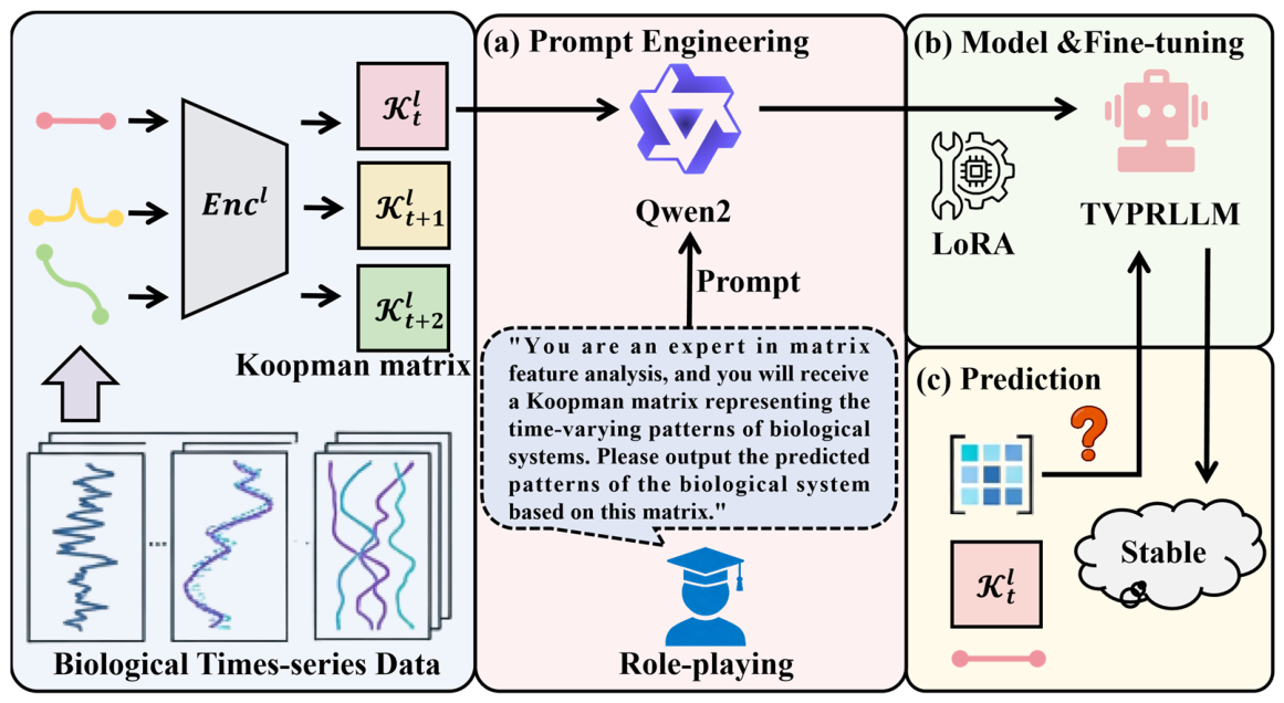
Liu et al. [10] demonstrated that the eigenvalues of the Koopman operator can characterize the frequency of dynamical evolution. Motivated by this finding, we propose a time-varying pattern recognition large language model, termed TVPRLLM, for pattern prediction in time-varying biologically related systems. Specifically, the model takes the Koopman matrix, which encodes the evolutionary characteristics of biologically related time-series data, as input and learns its features to infer the corresponding dynamic patterns. TVMILLM is designed for Koopman-guided time-varying pattern recognition and qualitative dynamical explanation, rather than autonomous biologically related mechanism discovery. As illustrated in Figure 3, TVPRLLM consists of three stages: prompt engineering, modeling and fine-tuning, and prediction.

2.4.1. Prompt Engineering

Prompts serve as task instructions for LLMs. Among various prompt engineering strategies, role-playing has become a widely adopted technique. By embedding a specific expert persona into the prompt, role-playing guides the LLM to perform the target task from a predefined professional perspective.
For a biologically related time-series sample, the Koopman transition matrix is denoted as K i R M × M , where i represents the i-th sample, and m denotes the dimension of the Koopman representation. Since large language models cannot directly receive floating-point matrices as continuous tensors, the Koopman matrix is first converted into a structured textual format. Before textualization, the matrix is normalized to reduce scale differences among samples:
K ~ i = K i μ i σ i + ϵ
where μ i and σ i denote the mean and standard deviation of the matrix elements, and ϵ is a small constant used to avoid division by zero. For relatively small Koopman matrices, the normalized matrix is serialized row by row. Each floating-point value is represented using a fixed decimal precision to two decimal places, and explicit delimiters are used to preserve the row-column structure.
Input: “[0.23, −1.02][0.87, 0.10]”.
When the Koopman matrix is large, directly serializing the entire matrix may produce an overly long prompt. Therefore, when the M > 8 , the eigenvalues of the Koopman matrix are used instead. The eigenvalues are sorted by descending magnitude. Eigenvalues are represented as scalar values. Each floating-point value is also represented using a fixed decimal precision to two decimal places. When the input exceeds the maximum length limit, the input text will be truncated. The eigenvalue-based textual representation is formatted as follows:
Input: “2.31 1.93 1.84 1.72 1.57 1.4 1.33 1.23”.
It should be noted that the textualization step does not assume that the LLM performs exact numerical linear algebra on the Koopman matrix. Instead, the Koopman matrix or its eigenvalues are regarded as compact dynamic descriptors of the original biologically related time-series. By converting these descriptors into a structured textual numerical format and applying supervised fine-tuning, the model learns task-specific associations between Koopman-derived numerical patterns and biologically related time-varying labels. To reduce information loss caused by textualization and tokenization, we normalize the matrix values, adopt a fixed numerical precision or scientific notation, and preserve the row-column structure using explicit delimiters.

2.4.2. Modeling and Fine-Tuning

TVPRLLM is built upon the Qwen2 LLM [15] and LoRA [33]. More specifically, TVPRLLM employs the pre-trained Transformer-based LLM Qwen2 as its base classifier. The model is then fine-tuned using the time-varying patterns extracted from the observed data, while LoRA is used to adapt the model to recognize and predict biologically related time-varying pattern labels. LoRA is a parameter-efficient fine-tuning approach that constrains updates of the weight matrices to a low-rank space. The effectiveness of TVPRLLM lies in its ability to leverage the extensive prior knowledge encoded in the pre-trained Qwen2 model.
For the input data K t l , if the Koopman matrix K t l is relatively small in scale, the entire matrix is directly used as input; otherwise, its eigenvalues are used instead. Since large language models can be fine-tuned for non-linguistic tasks without modifying their architecture or loss functions [34], the default cross-entropy loss [35] is adopted to fine-tune TVPRLLM. For each fine-tuning sample, the training template is defined as follows:
Prompt: “You are an expert in matrix feature analysis, and you will receive a Koopman matrix representing the time-varying patterns of biologically related systems. Please output the predicted patterns of the biologically related system based on this matrix.”
Input: “ K t l ”;
Output: “Stable”;

2.4.3. Prediction

After fine-tuning TVPRLLM, the model outputs binary classification results, such as “Increase” or “Reduce”, and “Chaos” or “Stable”, to represent the potential meaning state of the biologically related system.

3. Results

3.1. Experimental Details

Baselines: Six representative biologically related time-series-predicting methods were selected for performance comparison with our proposed TVNN: Vector Autoregressive Integrated Moving Average (VARIMA) [36]; Support Vector Regression (SVR) with radial basis function kernel [37]; Recurrent Neural Network (RNN) [38]; Koopman Autoencoder (KAE) [39]; Embedding, Koopman, and Autoencoder-based multi-omics Time-series Prediction model (EKATP) [3]; Koopman Predictor (Koopa) [10]; DLinear [40]; PatchTST [41]; iTransformer [42]; and TiDE [43].
Evaluation metrics: To quantitatively assess the prediction performance of different models, the Root-Mean-Square Error (RMSE) [32] was used as the evaluation metric:
R M S E = 1 L i = M + 1 m + L Z ^ i Z i 2 2
where Z i denotes the true value, Z ^ i denotes the predicted value, and L   is the prediction horizon.
Input data: For all datasets, the input variables were normalized using Min–Max normalization [44] prior to model training.
Key hyperparameters: Table 1 shows the key hyperparameter settings used in the main experiments. Without further explanation, all main results were obtained using the original Fourier frequency domain decomposition.

3.2. Experimental Results and Analysis on TVNN

To address our first scientific question, we compared the proposed TVNN with six representative methods: the widely used VARIMA, SVR, RNN, and KAE, as well as two recently developed models, EKATP and Koopa [10]. Subsequently, we investigated how the Fourier filter and the time-varying degree of biologically related systems affect the prediction performance of the TVNN model. Finally, the effectiveness of the Fourier frequency domain decomposition was demonstrated by ablation experiments.

3.2.1. Prediction of Biologically Related Time-Series Data

Table 2 summarizes the quantitative comparison results of multivariate prediction.
The first column lists six different datasets, including Proteomics, Gene, Solar, EMG, Climate, and ILI. Then, the table lists the performance of the evaluation metric RMSE for each model at different predictive time steps. The best average results are highlighted in bold. The winning counts show how many times each model achieves the best metric.
The following observations can be drawn from Table 2:
(1)
According to the winning counts in the last row of Table 2, TVNN achieves the highest number of best-performing cases among the compared methods. This indicates that TVNN has strong overall competitiveness in multivariate forecasting, although it is not the best method for every dataset and prediction horizon.
(2)
In biologically related time-series prediction, the TVNN generally achieves competitive or lower RMSE values compared with the Koopman-theory-based models KAE, EKATP, and Koopa [10] in many settings.
(3)
By contrast, the overall prediction performance of VARIMA and SVR is inferior to that of the Koopman-theory-based models. Their results are generally higher and less competitive across the evaluated datasets and prediction horizons.

3.2.2. Fourier Frequency Domain Decomposition

Table 3 summarizes the effects of the Fourier filter parameter α and the time-varying degree of the biologically related system on the predictive performance of the TVNN. The first column lists the values of the time-varying parameter   θ , the second column reports the Fourier filter parameter α , and the remaining columns present the corresponding RMSE statistics of prediction results, including the minimum (Min), maximum (Max), average (Avg), and variance (Var). The experiments were conducted on the Proteomics dataset with the noise level fixed at σ = 0 . To increase the time-varying degree of the data, θ 0 was set to [ 0.8 ,   1.6 ,   2.4 ] . For each value of θ 0 , α was set to [ 10 % ,   20 % , 30 % ] . The model was trained using the first 800-time steps and then used to predict the subsequent 96-time steps. Each combination of θ 0 and α was evaluated under five different random seeds.
The results in Table 3 indicate that both the Fourier filter parameter α and time-varying degree θ have a substantial impact on the predictive performance of the TVNN, as follows:
(1)
When the system exhibits a relatively low degree of time variation ( θ = 0.8 ), the average RMSE decreases as α increases. By contrast, when the system becomes highly time-varying ( θ = 2.4 ), the average RMSE first decreases and then increases with increasing α .
(2)
For a fixed α , as the time-varying degree θ increases from 0.8 to 2.4, the minimum, maximum, and average RMSE values all show an overall downward trend.
(3)
As θ increases from 0.8 to 2.4, the variance of RMSE generally decreases.
To further evaluate the sensitivity and stability of the proposed TVNN, we analyzed how the design of the frequency-domain decomposition affects forecasting accuracy and stability. Specifically, we compared the original Fourier masking strategy used in the released implementation with a symmetric low-pass decomposition across multiple values, forecast horizons, and random seeds.
To examine the sensitivity of the proposed TVNN framework to the design of the frequency-domain decomposition, we conducted an additional robustness analysis comparing two decomposition schemes: (1) the original Fourier masking strategy used in the public implementation and (2) a symmetric low-pass decomposition that preserves conjugate low-frequency pairs in the Fourier domain. The analysis was performed on the two synthetic dynamical systems released with the public codebase, namely, the Proteomics and Gene datasets.
For each dataset, we evaluated both decomposition variants under multiple values of the Fourier parameter [ 0.1 , 0.2 , 0.3 , 0.4 , 0.5 ] ; five random seeds; and forecast horizons of 16, 32, 48, and 64 steps. The training length was fixed at ( M = 1024 ), the segment length was set to ( M / S = 8 ), and all runs used the same optimization settings to ensure fair comparison. We report both the average RMSE and the standard deviation across seeds in order to characterize predictive accuracy and stability.
For Table 4 on the Proteomics dataset, the symmetric low-pass decomposition generally yielded better short- and medium-horizon forecasting performance than the original masking strategy, especially for moderate values of. For example, at (= 0.3), the corrected decomposition reduced the mean RMSE from 0.295 to 0.130 at horizon 16, from 0.322 to 0.216 at horizon 32, and from 0.366 to 0.277 at horizon 48. Similar improvements were observed at (= 0.4), indicating that the decomposition design materially affects predictive quality even on a relatively smooth nonlinear system.
For Table 4 on the Gene dataset, the influence of the decomposition was even more pronounced. Rather than producing a uniform performance shift, different combinations of decomposition strategy led to markedly different stability regimes. In some settings, the original masking strategy exhibited severe long-horizon divergence; for instance, at (= 0.2), the mean RMSE increased to 5130.975 at horizon 48 and 426,299,925.898 at horizon 64. Conversely, in other settings, the symmetric decomposition became unstable, such as at (= 0.5), where its mean RMSE rose sharply at longer horizons. These results indicate that the frequency decomposition is not merely a preprocessing detail, but a critical factor governing both predictive accuracy and numerical stability.
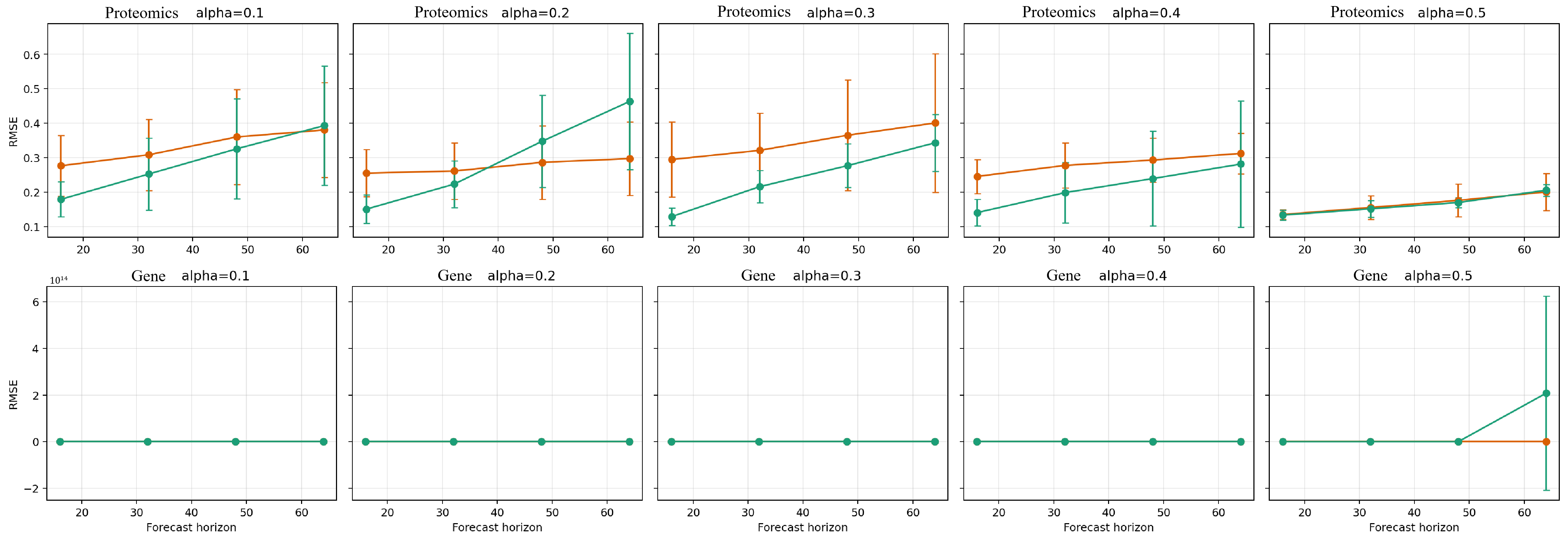
Figure 4 shows the forecasting RMSE versus prediction horizon under different Fourier parameters on the Proteomics dataset and Gene dataset. Error bars indicate standard deviation across five random seeds. The symmetric low-pass decomposition generally improves short- and medium-horizon performance, particularly at moderate values. The results reveal strong sensitivity of TVNN to the exact frequency decomposition and demonstrate that some decomposition settings lead to severe long-horizon instability.
Overall, the results in Table 3 demonstrate that TVNN achieves competitive predictive accuracy under the selected benchmark setting, confirming the effectiveness of the proposed model in predicting time-varying biological-related systems. Nevertheless, the robustness analysis over Fourier parameter values, forecast horizons, and random seeds in Table 4 and Figure 4 shows that the forecasting behavior of TVNN is highly sensitive to the precise form of Fourier decomposition. Therefore, the performance of TVNN, including its RMSE and long-horizon stability, should be interpreted as depending on the selected frequency-domain decomposition strategy, rather than as evidence of unconditional robustness across all possible masking designs. These findings indicate that the choice of decomposition should be explicitly justified, and robustness analyses should accompany any performance claim based on a single masking strategy.

3.2.3. Ablation Experiment

We further conducted ablation experiments to verify the effectiveness of the Fourier filter-based frequency-domain decomposition. Specifically, while keeping all other settings unchanged, we constructed both TVNNg using only the global prediction module and TVNNl using only the time-varying prediction module. Each model was then trained under five different random seeds. Finally, the average values of the predictive metric RMSE for the TVNN, TVNNg, and TVNNl are summarized in Table 5, where the best average results are highlighted in bold.
Table 5 shows that the TVNN achieves the best overall performance among the three models, indicating the benefit of jointly modeling global and time-varying dynamics in biologically related time-series prediction. To further examine the contribution of each component, we conducted a T-test [45] between the TVNN and its two ablated variants, TVNNg and TVNNl.
Compared with TVNN, TVNNg shows slightly higher RMSE values across the datasets; however, none of these differences are statistically significant (p > 0.05). Thus, the advantage of TVNN over TVNNg should be interpreted as a numerical improvement rather than statistically reliable evidence. TVNNl yields the highest RMSE values overall. The differences between TVNN and TVNNl are statistically significant in all cases except the Proteomics dataset with 16 prediction steps, where the p-value does not reach the significance threshold. These results indicate that the time-varying predictive module provides a more statistically supported contribution, while the global predictive module also contributes to reducing the average prediction error numerically.

3.3. Experimental Results and Analysis on TVPRLLM

To address the second scientific question, we first analyze the characteristics of biologically related time-varying patterns represented by the Koopman transition matrices. After that, we further recognize and classify these time-varying patterns with the aid of TVPRLLM.

3.3.1. Biologically Related Time-Varying Patterns

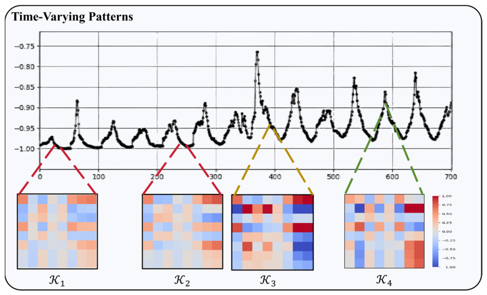
Figure 5 shows the heatmaps of the time-varying Koopman matrices ( K l ) at different periods on the influenza disease dataset. In the heatmaps, red, blue, and white indicate positive matrix values, negative matrix values, and zero values, respectively. The darker the color, the greater the magnitude of the corresponding matrix value.
It can be observed that the time-varying Koopman matrices ( K l ) exhibit distinctly different temporal patterns across different stages. Specifically, the heatmaps of ( K 1 ) and ( K 2 ) show strong overall similarity, with relatively small values that are more uniformly distributed. By contrast, the heatmap of ( K 3 ) contains more extreme large and small values. Likewise, the heatmap of ( K 4 ) includes many extreme values and shows a certain complementary trend with ( K 3 ).
This phenomenon can be explained by the fact that the sequences corresponding to ( K 1 ) and ( K 2 ) both display similar stable trends. As a result, the color variations in the heatmaps of ( K 1 ) and ( K 2 ) are relatively smooth, mainly consisting of light blue and light red, with only minor differences in intensity. By contrast, ( K 3 ) corresponds to a sharply decreasing sequence, so its heatmap exhibits more pronounced color changes. The dark red and dark blue regions indicate values with great absolute magnitudes. Likewise, the sequence represented by ( K 4 ) shows a steep upward trend, and its heatmap displays pronounced color variations with many dark red and dark blue areas. Furthermore, it can be observed that the heatmap of ( K 3 ) corresponding to a decreasing pattern and the heatmap of ( K 4 ) corresponding to an increasing pattern exhibit opposite sign relationships in the regions with large absolute values, as reflected by the reversed red–blue color distribution. Therefore, the time-varying Koopman matrices in the ILI dataset can, to some extent, reflect whether the disease incidence is in a decreasing or increasing phase during a specific period.

3.3.2. Time-Varying Pattern Recognition

To further explore the information contained in the time-varying Koopman matrices and investigate the states of biologically related time-varying systems at different stages, in this study, we systematically evaluate the effects of different Koopman matrix combinations on the accuracy of predicting the current state of biologically related time-varying systems based on the proposed TVPRLLM. Specifically, we examine the performance of the time-varying Koopman matrix ( K l ), the combination of the global Koopman matrix, and the time-varying Koopman matrix ( K g + K l ) in the state predictive task. F1-Score and AUPRC [46] are adopted as the evaluation metrics.
The proteomics dataset contains 450 samples, and the gene dataset also includes 450 samples. For each dataset, all samples are split into a training set and a test set, with a ratio of 70% and 30%, respectively. No additional validation set is used in this experiment. The model obtained after full training on the training set is used as the final model and is directly evaluated on the held-out test set.
The ground-truth labels are assigned based on the dynamic characteristics of the simulated systems. For the proteomics dataset generated by the nonlinear pendulum model, each segment is labeled as Increase or Reduce according to the sign of its temporal slope. This dataset is class-imbalanced, containing 96 positive samples, accounting for 21%, and 354 negative samples, accounting for 79%. For the gene dataset generated by the Lorenz model, labels are determined by the attractor state: samples located on the attractor are labeled as Stable, whereas those deviating from the attractor or exhibiting irregular dynamics are labeled as Chaos. The gene dataset is approximately class-balanced.
Since the proteomics dataset shows a clear class imbalance, we use both F1-Score and AUPRC to evaluate the classification performance. F1-Score measures the trade-off between precision and recall, while AUPRC is more suitable for evaluating predictive performance under imbalanced classification settings. These settings provide a clearer basis for interpreting the F1-Score and AUPRC results reported in Table 6.
Table 6 presents the predictive results of different Koopman matrix combinations to identify the current states of biologically related time-varying systems on the TVPRLLM, with the best average results highlighted in bold. The results show that, in both Proteomics and Gene domains, using only the time-varying Koopman matrix ( K l ) achieves the best predictive performance on both F1-Score and AUPRC. By contrast, after introducing the global Koopman matrix ( K g ), the predictive performance decreases under the ( K g + K l ) settings.
To further evaluate the statistical reliability of these differences, we conducted t-tests between the ( K l ) and ( K g + K l ) settings. The test results show that the predictive performance of TVPRLLM using only the time-varying Koopman matrix ( K l ) is significantly better than that under the ( K g + K l ) setting. This indicates that the time-varying Koopman matrix captures more discriminative dynamic patterns for biologically related state identification, whereas the introduction of the global Koopman matrix may partially obscure such time-varying information. Therefore, the LoRA fine-tuned TVPRLLM can effectively identify the time-varying patterns of biologically related systems encoded by Koopman matrices.
To justify the use of the LLM-based TVPRLLM for biological state prediction, we further compare it with two lightweight traditional classifiers, RF and MLP. All compared models use the same Koopman-derived dynamic information, but with model-specific input formats. For TVPRLLM, the time-varying Koopman matrix K l or its eigenvalues are converted into textualized inputs. For RF and MLP, the same information is provided as numerical feature vectors, where full Koopman matrices are flattened row by row, and eigenvalues are directly used as vector features. Therefore, the comparison is based on the same underlying dynamic information, with only the input format adapted to each model type. The datasets were split into training and test sets using the same ratio. All experiments were repeated four times with different random seeds. For RF and MLP, a limited grid search over commonly used hyperparameter ranges was conducted using only the training data, and the held-out test set was used only for final evaluation. The p-values were computed using paired t-tests across the four repeated runs, where each pair corresponded to the same train/test split used by TVPRLLM, RF, and MLP. In addition to F1-score, we report precision, recall, F1-score, and AUPRC to provide a more comprehensive evaluation under potentially imbalanced label distributions. The best results are highlighted in bold.
As shown in Table 7, TVPRLLM achieves the highest F1-scores on both the Proteomics and Gene datasets using the same Koopman-derived dynamic representations. On the Proteomics dataset, TVPRLLM obtains the best precision, recall, and F1-score, with an F1-score of 0.969 compared with 0.925 for RF and 0.904 for MLP. However, RF and MLP show higher AUPRC values, suggesting better ranking ability across thresholds. On the Gene dataset, TVPRLLM also achieves the highest F1-score, whereas RF and MLP obtain higher precision values, and MLP achieves the best AUPRC. The recall differences on Gene are not statistically significant.
The paired t-test results indicate that TVPRLLM’s F1-score improvements over RF and MLP are statistically significant on both datasets, although not all metric-wise differences are significant. TVPRLLM also shows smaller variances across repeated runs, suggesting better stability. Overall, these results indicate that TVPRLLM is effective and stable for biological state prediction from time-varying Koopman representations, particularly in terms of F1-score, while RF and MLP remain competitive in precision- and ranking-oriented metrics.

3.4. The Biologically Related Time-Series Data Predictive Platform

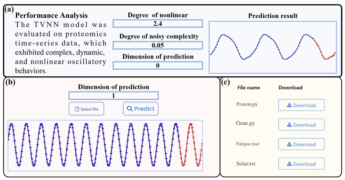
To answer our third scientific question, we developed an online predictive platform based on the TVNN model with three key functions: performance analysis, biologically related time-series data prediction, and data download. Figure 6a visually presents the predicted values and variation trends of proteomic time-series data, thereby helping users evaluate the accuracy and reliability of the TVNN model predictions. Figure 6b shows the predictive results generated by the TVNN model based on the user-input biologically related time series. Figure 6c presents the data download module, where users can click “Download” to obtain the data.
The prediction platform was developed using Django to provide online analysis and visualization of biologically related time-series data. It supports built-in datasets as well as external user-uploaded files. Users can select the target dimension and submit the data to the backend, where the trained TVNN model performs prediction automatically. The results are displayed as visualized prediction curves. By using the same input data and parameter settings, users can reproduce the prediction results.

4. Discussion

To address the challenges of biologically related time-series prediction, in this study, we propose a TVNN model that combines frequency-domain information with Koopman theory. Furthermore, we introduce TVPRLLM to recognize and classify hidden time-varying patterns in biologically related systems.
Specifically, a TVNN is developed to effectively extract the non-stationary characteristics of biologically related time-series data and model the nonlinear dynamical evolution of time-varying biologically related systems, thereby enabling accurate prediction of temporal shift data. Although Koopman-based forecasting, Fourier decomposition, and neural encoder–decoder architectures have been widely studied, the novelty of TVNN lies in integrating them for non-stationary, biologically related time-series modeling. TVNN first uses Fourier frequency-domain decomposition to separate different dynamic components of the input sequence. Then, instead of learning only a single global Koopman operator, TVNN constructs both a global predictive module and a time-varying predictive module. The global Koopman matrix captures the overall dynamic evolution of the system, while the time-varying Koopman matrices characterize local stage-specific dynamic changes. This design enables TVNN to capture both global system patterns and local non-stationary variations. Compared with EKATP, TVNN further incorporates frequency-domain decomposition and explicitly models time-varying Koopman transitions. Compared with Koopa, TVNN differs by introducing a dual Koopman structure composed of global and local time-varying predictive modules and by further using the learned time-varying Koopman matrices for downstream state recognition.
In addition, a large language model collaboratively fine-tuned with LoRA is employed to construct TVPRLLM, which is used to identify and classify time-varying patterns in biologically related systems. Comprehensive experiments conducted on multiple biologically related time-series datasets systematically validate the effectiveness of the proposed methods through model comparison, stability analysis, ablation studies, and time-varying pattern recognition experiments.
In terms of overall model performance, Table 2 shows that the TVNN achieves superior overall performance, indicating its stronger modeling capability to predict time-varying biologically related systems. The fact that the TVNN outperforms KAE, EKATP, and Koopa demonstrates that the collaborative design of the global prediction module and the time-varying prediction module can more effectively capture both global patterns and local time-varying dynamics in biologically related time-series data. The weaker performance of VARIMA and SVR suggests that traditional statistical and regression-based methods are not better than Koopman theory-based methods in handling nonlinear and strongly time-varying biologically related systems.
Table 3 reveals the role of Fourier-domain decomposition in the TVNN. When the system has a low degree of time variation, its evolution is dominated mainly by the Koopman operator associated with low-frequency global patterns. Therefore, increasing α appropriately increases the ability of the TVNN to extract global patterns, leading to improved predictive performance. By contrast, when the system is highly time-varying, its evolution is governed more by the Koopman operator associated with high-frequency time-varying patterns. In this case, moderately increasing α facilitates a more effective separation of global and time-varying components, thereby improving predictive accuracy. However, when α becomes excessively large, the proportion of retained time-varying components decreases, weakening the ability of the TVNN to characterize temporal dynamics and ultimately degrading predictive performance.
The ablation experiment results listed in Table 5 further confirm that the dynamics of time-varying biologically related systems depend on both global long-term trends and local time-varying changes. The global predictive module mainly models the overall evolutionary trend of the system, whereas the time-varying predictive module captures local dynamics and non-stationary characteristics. Because biologically related time-series data are typically highly time-varying, local changes have a more direct impact on prediction errors; therefore, removing the time-varying predictive module leads to a greater statistically significant performance drop. By contrast, when only the global predictive module is retained, the model can still capture the main evolutionary trend, so the performance degradation is relatively limited. Overall, the joint modeling of these two modules is essential for accurate biologically related time-series forecasting and further validates the effectiveness of the frequency-domain decomposition strategy.
The additional robustness experiments in Table 4 and Figure 4 indicate that the performance of TVNN is sensitive to the precise form of the Fourier decomposition. In particular, different masking strategies may lead not only to different average forecasting errors but also to qualitatively different stability regimes, especially on the Lorenz system.
Figure 5 shows that the time-varying Koopman matrix ( K l ) can effectively characterize the time-varying patterns of biologically related systems across different periods, as reflected by the variations in the heatmaps. To further explore the information contained in the time-varying Koopman matrices, Table 6 indicates that the proposed time-varying predictive module can more effectively capture the dynamic characteristics of biologically related time-varying systems, thereby increasing the predictive accuracy of the TVNN model. In addition, Table 6 indicates that the global Koopman matrix ( K g ) may obscure the discriminative features of time-varying patterns, as global information is insufficient in characterizing the temporal variability of biologically related systems.
Our reassessment of the released TVPRLLM benchmarks in Table 7 shows that Koopman-derived features already provide highly separable information for binary state recognition. Therefore, the current evidence supports a claim of strong feature discriminability more directly than a claim of uniquely LLM-enabled pattern recognition. Future work should compare LLM-based recognizers against stronger conventional baselines and use probability-based evaluation metrics consistently.
Overall, these findings indicate that our proposed framework not only improves predictive performance for biologically related time-series data in time-varying systems but also provides an effective way to recognize and classify hidden dynamic patterns.

5. Conclusions

In conclusion, the proposed TVNN effectively addresses biologically related time-series prediction in time-varying systems by combining frequency-domain decomposition with Koopman embedding theory. The experimental results demonstrate that the TVNN can successfully disentangle global evolutionary patterns and local time-varying dynamics, leading to superior predictive performance, robustness, and consistency across benchmark and real biologically related datasets. Furthermore, TVPRLLM provides a recognition-based approach for identifying the dynamic patterns captured by TVNN. The developed platform also offers a visual and user-friendly tool for biologically related time-series analysis and prediction, further facilitating the application of the proposed methods in systems biology [47].
Despite these promising results, several challenges remain, including the non-stationarity and heterogeneity of biologically related data, as well as the need for stronger pattern recognition capability and generalization across diverse datasets. Thus, our future work will focus on integrating richer biologically related prior knowledge, extending the framework to multimodal data, and further increasing model robustness and practical applicability in real-world biomedical research.

Author Contributions

Methodology, Y.Y., L.Z., and Y.J.; investigation, Y.Y., Y.J., and F.Z.; resources, Y.Y., M.X., and Y.J.; writing—original draft preparation, Y.Y. and Y.J.; validation, S.G.M., I.R.M.; writing—review and editing, Y.Y., L.Z., S.G.M., I.R.M.; supervision, M.X.; funding acquisition, F.Z. and L.Z. All authors have read and agreed to the published version of the manuscript.

Funding

This work was supported by grants from the National Natural Science Foundation of China [62372316]; Noncommunicable Chronic Diseases-National Science and Technology Major Project [2024ZD0532900]; Sichuan Science and Technology Program key project [2025YFHZ0066]; and Sichuan Science and Technology Program (2025NSFSC2088).

Institutional Review Board Statement

Not applicable.

Informed Consent Statement

Not applicable.

Data Availability Statement

The datasets and codes are publicly available on 25 May 2026 at https://github.com/347251369/Time-Varying-Biological-Time-Series-Prediction. The platform is available on 25 May 2026 at http://www.combio-lezhang.online/QCETBBTSPP/home/.

Acknowledgments

During the preparation of this manuscript, the authors used GPT-5.4 for the purposes of English translation and editing. The authors have reviewed and edited the output and take full responsibility for the content of this publication. The authors appreciate the contribution of Linjing Wei (College of Information Science and Technology, Gansu Agricultural University, Lanzhou 730000, China) and Jianzhou Lu (Gansu Haifeng Information Technology Co., Ltd., Lanzhou 730000, China) to this manuscript.

Conflicts of Interest

The authors declare no conflicts of interest.

References

  1. Lähnemann, D.; Köster, J.; Szczurek, E.; McCarthy, D.J.; Hicks, S.C.; Robinson, M.D.; Vallejos, C.A.; Campbell, K.R.; Beerenwinkel, N.; Mahfouz, A.; et al. Eleven grand challenges in single-cell data science. Genome Biol. 2020, 21, 31. [Google Scholar] [CrossRef]
  2. Li, W.; Yang, X.; Liu, W.; Xia, Y.; Bian, J. DDG-DA: Data Distribution Generation for Predictable Concept Drift Adaptation. Proc. AAAI Conf. Artif. Intell. 2022, 36, 4092–4100. [Google Scholar] [CrossRef]
  3. Liu, S.; You, Y.; Tong, Z.; Zhang, L. Developing an Embedding, Koopman and Autoencoder Technologies-Based Multi-Omics Time Series Predictive Model (EKATP) for Systems Biology research. Front. Genet. 2021, 12, 761629. [Google Scholar] [CrossRef]
  4. Chen, C.; Li, R.; Shu, L.; He, Z.; Wang, J.; Zhang, C.; Ma, H.; Aihara, K.; Chen, L. Predicting future dynamics from short-term time series using an Anticipated Learning Machine. Natl. Sci. Rev. 2020, 7, 1079–1091. [Google Scholar] [CrossRef]
  5. Wu, T.; Gao, X.; An, F.; Sun, X.; An, H.; Su, Z.; Gupta, S.; Gao, J.; Kurths, J. Predicting multiple observations in complex systems through low-dimensional embeddings. Nat. Commun. 2024, 15, 2242. [Google Scholar] [CrossRef] [PubMed]
  6. Masarotto, G. Bootstrap prediction intervals for autoregressions. Int. J. Forecast. 1990, 6, 229–239. [Google Scholar] [CrossRef]
  7. Box, G.E.; Pierce, D.A. Distribution of residual autocorrelations in autoregressive-integrated moving average time series models. J. Am. Stat. Assoc. 1970, 65, 1509–1526. [Google Scholar] [CrossRef]
  8. Kim, T.; Kim, J.; Tae, Y.; Park, C.; Choi, J.-H.; Choo, J. Reversible Instance Normalization for Accurate Time-Series Forecasting against Distribution Shift. In Proceedings of the International Conference on Learning Representations, Online, 25–29 April 2022. [Google Scholar]
  9. Koopman, B.O. Hamiltonian Systems and Transformation in Hilbert Space. Proc. Natl. Acad. Sci. USA 1931, 17, 315–318. [Google Scholar] [CrossRef] [PubMed]
  10. Liu, Y.; Li, C.; Wang, J.; Long, M. Koopa: Learning Non-stationary Time Series Dynamics with Koopman Predictors. In Proceedings of the Conference and Workshop on Neural Information Processing Systems, New Orleans, LA, USA, 10–16 December 2023. [Google Scholar]
  11. Zhou, T.; Ma, Z.; Wang, X.; Wen, Q.; Sun, L.; Yao, T.; Yin, W.; Jin, R. FiLM: Frequency improved Legendre Memory Model for Long-term Time Series Forecasting. In Proceedings of the Conference and Workshop on Neural Information Processing Systems, New Orleans, LA, USA, 28 November–9 December 2022. [Google Scholar]
  12. Yi, K.; Zhang, Q.; Fan, W.; Wang, S.; Wang, P.; He, H.; An, N.; Lian, D.; Cao, L.; Niu, Z. Frequency-domain MLPs are More Effective Learners in Time Series Forecasting. In Proceedings of the Conference and Workshop on Neural Information Processing Systems, New Orleans, LA, USA, 10–16 December 2023. [Google Scholar]
  13. Wang, R.; Dong, Y.; Arik, S.Ö.; Yu, R. Koopman Neural Operator Forecaster for Time-series with Temporal Distributional Shifts. In Proceedings of the International Conference on Learning Representations, Kigali, Rwanda, 1–5 May 2023. [Google Scholar]
  14. Jiang, Z.; Cheng, D.; Qin, Z.; Gao, J.; Lao, Q.; Ismoilovich, A.B.; Gayrat, U.; Elyorbek, Y.; Habibullo, B.; Tang, D.; et al. TV-SAM: Increasing Zero-Shot Segmentation Performance on Multimodal Medical Images Using GPT-4 Generated Descriptive Prompts Without Human Annotation. Big Data Min. Anal. 2024, 7, 1199–1211. [Google Scholar] [CrossRef]
  15. Yang, A.; Yang, B.; Hui, B.; Zheng, B.; Yu, B.; Zhou, C.; Li, C.; Li, C.; Liu, D.; Huang, F.; et al. Qwen2 Technical Report. arXiv 2024, arXiv:2407.10671. [Google Scholar] [CrossRef]
  16. Heryanto, Y.D.; Zhang, Y.-Z.; Imoto, S. Predicting cell types with supervised contrastive learning on cells and their types. Sci. Rep. 2024, 14, 430. [Google Scholar] [CrossRef] [PubMed]
  17. Tyanova, S.; Temu, T.; Sinitcyn, P.; Carlson, A.; Hein, M.Y.; Geiger, T.; Mann, M.; Cox, J. The Perseus computational platform for comprehensive analysis of (prote)omics data. Nat. Methods 2016, 13, 731–740. [Google Scholar] [CrossRef]
  18. Mias, G.I.; Yusufaly, T.; Roushangar, R.; Brooks, L.R.; Singh, V.V.; Christou, C. MathIOmica: An Integrative Platform for Dynamic Omics. Sci. Rep. 2016, 6, 37237. [Google Scholar] [CrossRef]
  19. Anzel, A.; Heider, D.; Hattab, G. MOVIS: A multi-omics software solution for multi-modal time-series clustering, embedding, and visualizing tasks. Comput. Struct. Biotechnol. J. 2022, 20, 1044–1055. [Google Scholar] [CrossRef]
  20. Chen, P.; Liu, R.; Aihara, K.; Chen, L. Autoreservoir computing for multistep ahead prediction based on the spatiotemporal information transformation. Nat. Commun. 2020, 11, 4568. [Google Scholar] [CrossRef]
  21. Bertalan, T.; Dietrich, F.; Mezić, I.; Kevrekidis, I.G. On learning Hamiltonian systems from data. Chaos Interdiscip. J. Nonlinear Sci. 2019, 29, 121107. [Google Scholar] [CrossRef]
  22. Greydanus, S.; Dzamba, M.; Yosinski, J. Hamiltonian Neural Networks. In Proceedings of the Conference and Workshop on Neural Information Processing Systems, Vancouver, BC, Canada, 8–14 December 2019; pp. 15353–15363. [Google Scholar]
  23. Smale, S. Differential Equations, Dynamical Systems, and Linear Algebra; Academic press: Cambridge, MA, USA, 1974; Volume 60. [Google Scholar]
  24. Gökçe, A. A Mathematical Modeling Approach to Analyse the Effect of Additional Food in a Predator-Prey Interactions with a White Gaussian Noise in Prey’s Growth Rate. Int. J. Appl. Comput. Math. 2022, 8, 21. [Google Scholar] [CrossRef]
  25. Axtmann, G.; Rist, U. Scalability of OpenFOAM with large eddy simulations and DNS on high-performance systems. In High Performance Computing in Science and Engineering’ 16: Transactions of the High Performance Computing Center, Stuttgart (HLRS) 2016; Springer: Berlin/Heidelberg, Germany, 2016; pp. 413–424. [Google Scholar]
  26. Lorenz, E.N. Predictability: A problem partly solved. In ECMWF Seminar Proceedings I; 1995; Volume 1, Available online: https://www.ecmwf.int/en/elibrary/75462-predictability-problem-partly-solved (accessed on 21 May 2026).
  27. Lai, G.; Chang, W.-C.; Yang, Y.; Liu, H. Modeling Long- and Short-Term Temporal Patterns with Deep Neural Networks. In Proceedings of the 41st International ACM SIGIR Conference, Ann Arbor, MI, USA, 8–12 July 2018; pp. 95–104. [Google Scholar]
  28. Ou, J.; Li, N.; He, H.; He, J.; Zhang, L.; Jiang, N. Detecting muscle fatigue among community-dwelling senior adults with shape features of the probability density function of sEMG. J. Neuroeng. Rehabil. 2024, 21, 196. [Google Scholar] [CrossRef] [PubMed]
  29. Wu, H.; Xu, J.; Wang, J.; Long, M. Autoformer: Decomposition Transformers with Auto-Correlation for Long-Term Series Forecasting. In Proceedings of the Conference and Workshop on Neural Information Processing Systems, Vancouver, BC, Canada, 6–14 December 2021; pp. 22419–22430. [Google Scholar]
  30. Lin, S.; Lin, W.; Wu, W.; Zhao, F.; Mo, R.; Zhang, H. SegRNN: Segment Recurrent Neural Network for Long-Term Time Series Forecasting. arXiv 2023, arXiv:2308.11200. [Google Scholar] [CrossRef]
  31. Schmid, P.J. Dynamic mode decomposition of numerical and experimental data. J. Fluid Mech. 2010, 656, 5–28. [Google Scholar] [CrossRef]
  32. Hyndman, R.J.; Koehler, A.B. Another look at measures of forecast accuracy. Int. J. Forecast. 2006, 22, 679–688. [Google Scholar] [CrossRef]
  33. Hu, E.J.; Shen, Y.; Wallis, P.; Allen-Zhu, Z.; Li, Y.; Wang, S.; Wang, L.; Chen, W. LoRA: Low-Rank Adaptation of Large Language Models. In Proceedings of the International Conference on Learning Representations, Virtual Event, 25–29 April 2022. [Google Scholar]
  34. Dinh, T.; Zeng, Y.; Zhang, R.; Lin, Z.; Gira, M.; Rajput, S.; Sohn, J.-y.; Papailiopoulos, D.; Lee, K. LIFT: Language-Interfaced Fine-Tuning for Non-language Machine Learning Tasks. In Proceedings of the Conference and Workshop on Neural Information Processing Systems, New Orleans, LA, USA, 28 November–9 December 2022; Volume 35, pp. 11763–11784. [Google Scholar]
  35. Kline, D.M.; Berardi, V.L. Revisiting squared-error and cross-entropy functions for training neural network classifiers. Neural Comput. Appl. 2005, 14, 310–318. [Google Scholar] [CrossRef]
  36. Ridenhour, B.J.; Brooker, S.L.; Williams, J.E.; Van Leuven, J.T.; Miller, A.W.; Dearing, M.D.; Remien, C.H. Modeling time-series data from microbial communities. ISME J. 2017, 11, 2526–2537. [Google Scholar] [CrossRef]
  37. Ma, X.; Zhang, Y.; Wang, Y. Performance evaluation of kernel functions based on grid search for support vector regression. In Proceedings of the 7th International Conference on Cybernetics and Intelligent Systems, CIS 2015, and IEEE Conference on Robotics, Automation and Mechatronics, Siem Reap, Cambodia, 15–17 July 2015; pp. 283–288. [Google Scholar]
  38. Jiang, J.; Lai, Y.-C. Model-free prediction of spatiotemporal dynamical systems with recurrent neural networks: Role of network spectral radius. Phys. Rev. Res. 2019, 1, 033056. [Google Scholar] [CrossRef]
  39. Azencot, O.; Erichson, N.B.; Lin, V.; Mahoney, M.W. Forecasting Sequential Data Using Consistent Koopman Autoencoders. In Proceedings of the 37th International Conference on Machine Learning, Virtual, 13–18 July 2020; pp. 475–485. [Google Scholar]
  40. Zeng, A.; Chen, M.; Zhang, L.; Xu, Q. Are Transformers Effective for Time Series Forecasting? In Proceedings of the Thirty-Seventh AAAI Conference on Artificial Intelligence, Washington, DC, USA, 7–14 February 2023; pp. 11121–11128. [Google Scholar]
  41. Nie, Y.; Nguyen, N.H.; Sinthong, P.; Kalagnanam, J. A Time Series is Worth 64 Words: Long-term Forecasting with Transformers. In Proceedings of the Eleventh International Conference on Learning Representations, Kigali, Rwanda, 1–5 May 2023. [Google Scholar]
  42. Liu, Y.; Hu, T.; Zhang, H.; Wu, H.; Wang, S.; Ma, L.; Long, M. iTransformer: Inverted Transformers Are Effective for Time Series Forecasting. In Proceedings of the Twelfth International Conference on Learning Representations, Vienna, Austria, 7–11 May 2024. [Google Scholar]
  43. Das, A.; Kong, W.; Leach, A.; Mathur, S.; Sen, R.; Yu, R. Long-term Forecasting with TiDE: Time-series Dense Encoder. In Trans. Mach. Learn. Res.; 2023; Volume 2023, Available online: https://arxiv.org/abs/2304.08424 (accessed on 21 May 2026).
  44. Gopal Krishna Patro, S.; Sahu, K.K. Normalization: A Preprocessing Stage. arXiv 2015, arXiv:1503.06462. [Google Scholar] [CrossRef]
  45. Jiang, Z.K.; Dai, W.; Wei, Q.; Qin, Z.Y.; Wei, R.; Li, M.Y.; Chen, X.L.; Huo, Y.; Liu, J.Y.; Li, K.; et al. Diffusion Model-Based Multi-Channel EEG Representation and Forecasting for Early Epileptic Seizure Warning. Interdiscip. Sci.-Comput. Life Sci. 2025. [Google Scholar] [CrossRef] [PubMed]
  46. Li, B.; Xiao, X.; Zhang, C.; Xiao, M.; Zhang, L. DGHNN: A deep graph and hypergraph neural network for pan-cancer related gene prediction. Bioinformatics 2025, 41, btaf379. [Google Scholar] [CrossRef]
  47. Hayat, M.; Aramvith, S. Superpixel-Guided Graph-Attention Boundary GAN for Adaptive Feature Refinement in Scribble-Supervised Medical Image Segmentation. IEEE Access 2025, 13, 196654–196668. [Google Scholar] [CrossRef]
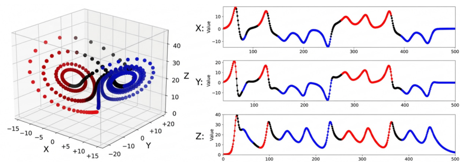
Figure 1. Lorenz system with different time-varying patterns and the temporal evolutions of its three state variables (X, Y, and Z).
Technologies 14 00321 g001
Figure 2. The time-varying neural network is composed of four parts: (a) data segmentation and decomposition; (b) global prediction module; (c) time-varying predictive module and (d) combination module.
Technologies 14 00321 g002
Figure 3. The TVPRLLM workflow, which consists of three steps: prompt engineering, modeling and fine-tuning, and prediction.
Technologies 14 00321 g003
Figure 4. TVNN forecasting robustness on the Proteomics dataset and Gene dataset.
Technologies 14 00321 g004
Figure 5. Time-varying Koopman matrix heatmaps on ILI dataset.
Technologies 14 00321 g005
Figure 6. The biologically related time-series data predictive platform. (a) The performance analysis module; (b) the biologically related time-series data prediction module; (c) the data download module.
Technologies 14 00321 g006
Table 1. Key hyperparameter settings used in the main experiments.
OptimizerLearning Rate (TVNN) Segments   Length   M / S Embedding Dimension   d Parameter   α [ λ g i d , λ g , λ l i d , λ l , λ c o n ] LoRA RankLearning Rate
(TVPRLLM)
AdamW 10 2 ~ 10 4 8 2 D 0.3 [ 0.1 , 0.1 , 0.3 , 0.4 , 0.1 ] 161 × 10−4
Table 2. The prediction results of prediction models on six time-series datasets.
DatasetsStepsTVNNVARIMASVRRNNKAEEKATPKoopaDLinearPatchTSTiTransformerTiDE
Proteomics160.07400.08620.07760.08670.07650.06310.06720.08410.06420.06740.0811
320.07520.07930.43850.09010.07970.07650.07720.08230.10180.12630.1140
480.07490.07580.35800.09280.08350.08170.07190.08220.10780.08510.1327
Gene80.18980.24783.0700.33960.59790.24120.19010.1026 0.11920.09650.3283
160.15960.38742.1710.38050.78110.26270.18430.35310.65930.20120.2524
240.19800.36371.7730.45580.95720.35940.24110.31190.81700.25520.3428
Solar320.64680.89871.65310.53711.61920.83280.44151.96321.41471.15791.6956
640.48310.94891.41520.47761.85980.76870.5753 2.50471.40250.88600.9277
960.44651.12461.45490.44481.82470.66230.54221.98370.60060.65300.7888
EMG160.29500.42180.34520.44130.43290.43780.30240.33970.45210.34770.4333
320.33830.43340.24410.45270.44320.44890.32410.37430.43390.36020.3440
480.30360.45230.19930.41280.40240.40870.28190.32640.67840.30600.3188
Climate160.01070.01121.00370.01340.01130.00960.09810.08570.10660.15740.0475
320.01250.01330.74200.01570.01850.01590.11320.17010.25950.57920.0676
480.01310.02210.60580.01900.01620.01950.12580.49670.22470.33710.1110
ILI80.12490.63040.74570.14710.13750.13821.12910.35630.29770.26920.1600
120.12320.62530.52730.17120.15190.12251.3238 0.21890.20160.45390.0786
160.13980.64120.37290.23870.13850.14931.43971.27911.48800.10350.0702
Winning counts80210220012
Table 3. The impact of Fourier filter parameter α and time-varying degree θ on the predictive performance of the TVNN model.
θ α RMSE
MinMaxAvgVar
0.810%0.08520.17910.1098 1.557 × 10 3
20%0.04170.12790.0821 1.860 × 10 3
30%0.04440.06130.0481 5.462 × 10 5
1.610%0.05010.12030.0815 7.546 × 10 4
20%0.04750.53670.1557 4.544 × 10 2
30%0.03080.10200.0552 7.989 × 10 4
2.410%0.00120.00810.0033 7.692 × 10 6
20%0.00150.00350.0023 7.939 × 10 7
30%0.00140.00540.0031 3.092 × 10 6
Table 4. Representative forecasting results from the Fourier robustness atlas. Results are averaged over five random seeds. The comparison shows that the precise Fourier masking strategy materially affects both RMSE and long-horizon stability.
DatasetAlphaFilter16 Steps32 Steps48 Steps64 Steps
Proteomics0.3Original0.2950.3220.3660.401
Symmetric low-pass0.1300.2160.2770.344
0.4Original0.2460.2780.2940.313
Symmetric low-pass0.1410.1990.2400.282
Gene0.2Original0.4300.6375130.975426,299,925.898
Symmetric low-pass0.6740.7001.1103.739
0.4Original0.6424.619231.63614,762.826
Symmetric low-pass0.5121.6145.51119.837
Table 5. The ablation experiments on the TVNN model.
DatasetsTVNNTVNNgTVNNl
RMSEp-ValueRMSEp-ValueRMSEp-Value
Proteomics
(16 Steps)
6.431   ×   10 2   ±     7.045   ×   10 5 6.876   ×   10 2   ±   1.941   ×   10 4 3.054   ×   10 1 7.641   ×   10 2   ±   3.197   ×   10 4 1.171   ×   10 1
Proteomics
(48 Steps)
6.723   ×   10 2     ±     5.823   ×   10 5 6.920   ×   10 2   ±   1.378   ×   10 4 3.680   ×   10 1 7.747   ×   10 2   ±   1.748   ×   10 4 4.876   ×   10 2
Gene
(16 Steps)
1.695   ×   10 1     ±     3.229   ×   10 4 1.795   ×   10 1   ±   1.273   ×   10 4 1.119   ×   10 1 3.556   ×   10 1   ±   1.759   ×   10 2 1.590   ×   10 2
Climate
(16 Steps)
9.963   ×   10 3     ±     4.405   ×   10 6 1.078   ×   10 2   ±   2.823   ×   10 7 1.590   ×   10 1 1.217   ×   10 2   ±   4.978   ×   10 6 2.428   ×   10 2
Climate
(32 Steps)
1.173   ×   10 2     ±     3.007   ×   10 6 1.247   ×   10 2   ±   8.692   ×   10 8 1.692   ×   10 1 1.589   ×   10 2   ±   7.777   ×   10 6 1.800   ×   10 2
Table 6. The predictive results of different Koopman matrices on TVPRLLM.
Datasets K l K g +   K l
F1-ScoreAUPRCF1-ScoreAUPRC
Ave ± Varp-ValueAve ± Varp-ValueAve ± Varp-ValueAve ± Varp-Value
Proteomics 0.969   ±   1.2  × 10−5 0.943   ±   4.5  × 10−5 0.163 ± 0.003 4.23  × 10−5 0.223 ± 4.8 e 4 2.19   ×   10 6
Gene 0.781   ±   0.001 0.659   ±   0.003 0.577 ± 0.016 0.041 0.479 ± 0.008 0.040
Table 7. The predictive results of K l matrices on TVPRLLM, RF and MLP.
DatasetsTVPRLLMRFMLP
Metricsp-ValueMetricsp-ValueMetricsp-Value
ProteomicsPrecision 0.950   ±   1.5  × 10−5 0.916   ±   1.0  × 10−1 2.08  × 10−2 0.905   ±   7.4  × 10−2 9.28  × 10−5
Recall 0.998   ±   4.0  × 10−6 0.94   ±   6.1  × 10−2 2.81  × 10−8 0.908   ±   7.3  × 10−2 1.55  × 10−11
F1 0.969   ±   1.2  × 10−5 0.925   ±   7.2  × 10−2 4.61  × 10−5 0.904   ±   5.8  × 10−2 1.55  × 10−10
AUPRC 0.943   ±   4.5  × 10−5 0.975   ±     4.3  × 10−2 2.43  × 10−5 0.971   ±   2.8  × 10−2 8.26  × 10−6
GenePrecision 0.629   ±   2.9  × 10−3 0.708   ±     1.8  × 10−1 3.83  × 10−2 0.722   ±     2.6  × 10−1 4.26  × 10−2
Recall 0.750   ±   3.3  × 10−2 0.773   ±     2.0  × 10−1 8.00  × 10−1 0.759   ±   3.0  × 10−1 9.25  × 10−1
F1 0.781   ±   1.0  × 10−3 0.732   ±   3.1  × 10−2 2.26  × 10−2 0.712   ±   6.1  × 10−2 3.68  × 10−3
AUPRC 0.659   ±   3.0  × 10−3 0.682   ±   1.1  × 10−1 4.25  × 10−1 0.853   ±   1.2  × 10−1 1.35  × 10−4
Disclaimer/Publisher’s Note: The statements, opinions and data contained in all publications are solely those of the individual author(s) and contributor(s) and not of MDPI and/or the editor(s). MDPI and/or the editor(s) disclaim responsibility for any injury to people or property resulting from any ideas, methods, instructions or products referred to in the content.