Lightweight Deep Learning Surrogates for ERA5-Based Solar Forecasting: An Accuracy–Efficiency Benchmark in Complex Terrain

Abstract

Accurate solar forecasting is critical for photovoltaic integration, particularly in regions with complex terrain and limited observations. This study benchmarks five deep learning architectures—MLP, RNN, LSTM, CNN, and a Grey Wolf Optimizer–enhanced MLP (MLP–GWO)—to evaluate the accuracy–computational efficiency trade-off for generating daily solar potential maps from ERA5 reanalysis over Mexico. Models were trained using a strict temporal split on a high-dimensional grid (85 × 129 points, flattened to 10,965 outputs) and evaluated in terms of predictive skill and hardware cost. The RNN achieved the best overall performance (RMSE ≈ 32.3, MAE ≈ 27.8, R² ≈ 0.96), while the MLP provided a competitive lower-complexity alternative (RMSE ≈ 54.8, MAE ≈ 46.0, R² ≈ 0.88). In contrast, the LSTM and CNN showed poorer generalization, and the MLP–GWO failed to converge. For the CNN, this underperformance is linked to the intentionally flattened spatial representation. Overall, the results indicate that within a specific ERA5-based, daily-resolution, and resource-constrained experimental framework, lightweight architectures such as RNNs and MLPs offer the most favorable balance between accuracy and computational efficiency. These findings position them as efficient surrogates of ERA5-derived daily solar potential suitable for large-scale, preliminary energy planning applications.

1. Introduction

In addition to data limitations, forecasting solar radiation is challenging because of large temporal and spatial variations driven by clouds, aerosols, and atmospheric patterns. Traditional statistical methods, such as autoregressive models and empirical formulas, often fail to capture complex, nonlinear relationships, especially at daily time scales [1,2]. Consequently, there has been a shift towards deep learning (DL) methods, which are well-suited for modeling the complex, nonlinear relationships between atmospheric predictors and solar radiation.

A wide range of neural network architectures have been explored for solar radiation forecasting, including multilayer perceptrons (MLPs), recurrent neural networks (RNNs), long short-term memory networks (LSTMs), and convolutional neural networks (CNNs). These models generally outperform traditional statistical methods for both solar radiation and photovoltaic power forecasting [3,4,5]. However, they differ substantially in architectural complexity and computational requirements: MLPs are relatively simple and efficient; RNNs and LSTMs are designed to capture temporal dependencies but incur higher computational cost; and CNNs are, in principle, well-suited for detecting spatial patterns in gridded data such as reanalysis products.

More complex or hybrid deep learning models have also been proposed, but they often require substantial computing power, memory, and training time [2,3,4]. Importantly, increasing model complexity does not necessarily lead to substantially better predictions when the input data have limited spatial resolution and known biases, as is the case for global reanalysis products. While complex architectures often prioritize accuracy, they frequently overlook the accuracy–efficiency trade-off, which is critical for deployment in resource-constrained environments. Therefore, benchmarking predictive accuracy together with computational cost is essential for practical adoption.

As an alternative pathway to improve neural network performance while controlling model complexity, metaheuristic optimization methods have been proposed. The Grey Wolf Optimizer (GWO) has been reported to be effective for training and tuning multilayer perceptrons in a range of regression problems, achieving competitive predictive performance without relying exclusively on gradient-based optimization [5]. However, it remains unclear whether such optimization strategies provide sufficient performance gains to offset their additional computational cost when applied to solar radiation forecasting using coarse-resolution reanalysis data.

Two hypotheses guide the evaluation. First (H1), lightweight models such as MLPs and vanilla RNNs can achieve a predictive performance comparable to more complex architectures (LSTMs and CNNs) at substantially lower computational cost. Second (H2), metaheuristic optimization strategies such as the Grey Wolf Optimizer (GWO), while conceptually appealing, may not yield sufficient performance gains to justify their additional computational burden in high-dimensional spatiotemporal forecasting tasks. Importantly, the observed underperformance of the MLP–GWO model is interpreted not as an implementation failure, but as a structurally informative result within the constraints of the present experimental setup and data characteristics. It reflects the challenges metaheuristic optimizers face when applied to high-dimensional, noisy regression problems with large output spaces—conditions under which gradient-based optimization retains a fundamental advantage. This interpretation is developed in depth in Section 4.

2. Materials and Methods

2.1. Study Area

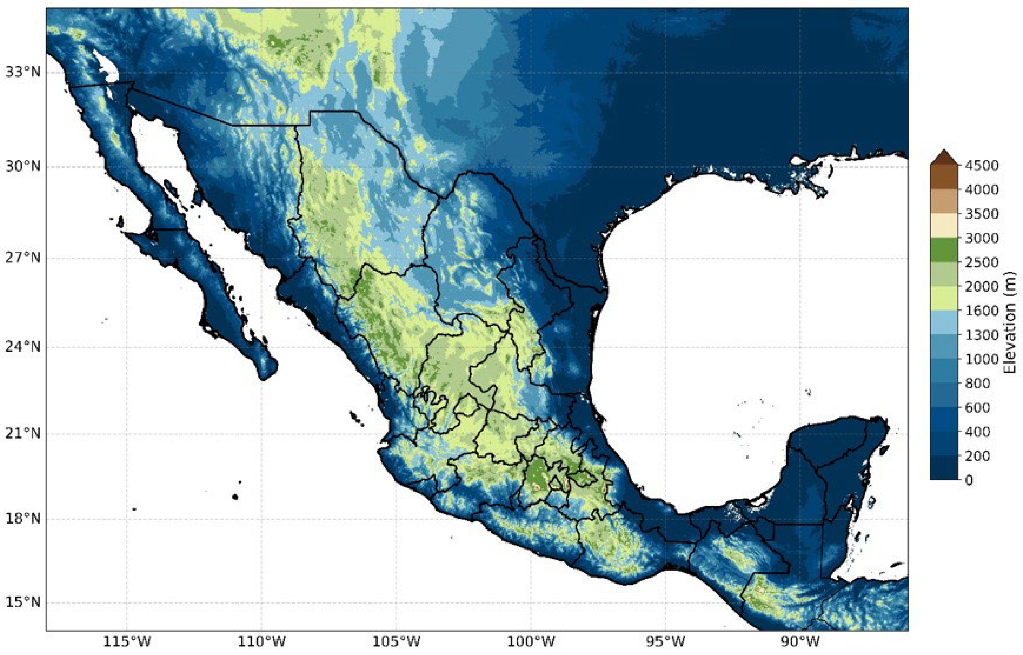
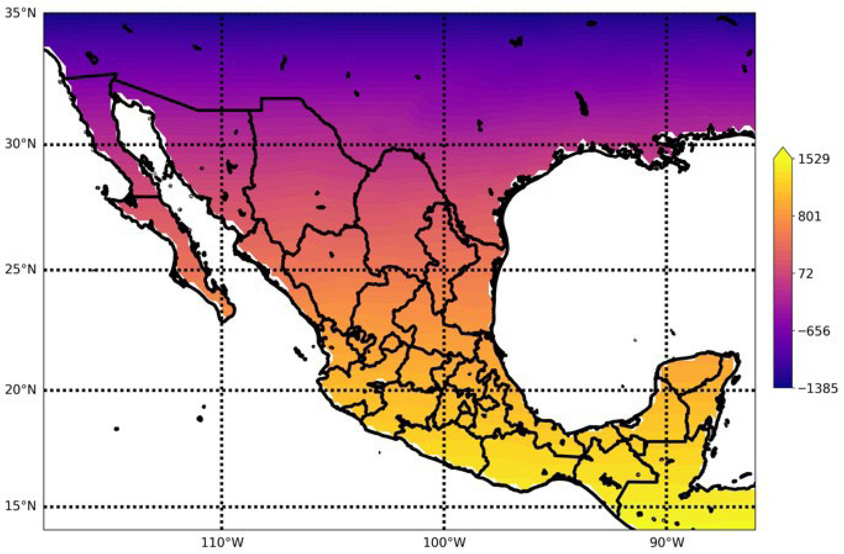
The study area encompasses the entire territory of Mexico, discretized on the native ERA5 grid between latitudes 14° N–35° N and longitudes 118° W–86° W. This domain constitutes a demanding testbed for solar radiation forecasting due to its pronounced topographic and climatic heterogeneity. It is dominated by major mountain systems—such as the Sierra Madre Occidental, the Sierra Madre Oriental, and the Trans-Mexican Volcanic Belt—with local elevation gradients exceeding 3000 m, which contrast sharply with extensive lowland coastal plains (Figure 1).

This complex orography, combined with diverse climatic regimes ranging from arid and semi-arid conditions in northern Mexico to humid tropical environments in the south, induces strong spatial variability in cloud cover and surface solar irradiance. Consequently, the region poses a significant challenge for predictive models based on moderate-resolution reanalysis data (~0.25°), such as ERA5, where sub-grid-scale topographic effects and mesoscale atmospheric circulations are not explicitly resolved. These limitations can result in systematic spatial smoothing and regional biases in surface radiation estimates, as documented in previous assessments [6,7].

2.2. Target Variable: Daily Solar Potential Based on ERA5

The primary data source for this study was the ERA5 fifth-generation global atmospheric reanalysis, produced by the European Center for Medium-Range Weather Forecasts (ECMWF) and distributed through the Copernicus Climate Change Service (C3S) [8]. ERA5 provides hourly, physically consistent estimates of surface and atmospheric variables at a native spatial resolution of 0.25° × 0.25°, offering a homogeneous and globally available dataset suitable for data-driven solar resource modeling.

All variables were retrieved from the consolidated ERA5 reanalysis product for the period January 1970 to December 2023. To extend the evaluation to the most recent conditions, preliminary near-real-time ERA5 update data were incorporated for the period January 2024 to June 2025. This combined strategy ensures both long-term climatological coverage and relevance for present-day forecasting applications.

Although ERA5 is available from 1950 onward, the analysis was restricted to data from January 1970. The pre-satellite period (1970–1978) was intentionally retained to increase the size of the training dataset and expose the models to a broader range of climatological variability. Despite the lower observational density prior to 1979, ERA5 maintains physical consistency through variational data assimilation and numerical model constraints, making it suitable for long-term statistical learning applications [9,10].

To ensure a realistic and operationally meaningful evaluation, the dataset was divided using a strict chronological split into three non-overlapping subsets:

• Training set: 1 January 1970 to 31 December 2008 (39 years);
• Validation set: 1 January 2009 to 31 December 2019 (11 years);
• Test set: 1 January 2020 to 30 June 2025 (5.5 years).

The target variable, referred to as daily solar potential Ps(t), was defined as the surface global horizontal irradiance (GHI). It was derived directly from the ERA5 Surface Solar Radiation Downwards (SSRD) variable, which represents the cumulative shortwave radiative energy flux (J m⁻²) incident on a horizontal surface.

For each calendar day $t$, the daily solar potential was computed by aggregating hourly SSRD values and converting them to standard photovoltaic energy units as follows:

$$Ps\left(t\right)={\displaystyle \frac{{\sum }_{i=1}^{N_h}SSR{D}_i\left(t\right)}{3.6 \times {10}^6}}\left(\mathrm{k}\mathrm{W}\mathrm{h}·{\mathrm{m}}^{-2}·\mathrm{d}\mathrm{a}{\mathrm{y}}^{-1}\right)$$

(1)

where $N_h$ denotes the number of hourly records per day (typically 24), and the divisor converts joules to kilowatt-hours. This formulation provides a physically consistent and reproducible proxy for daily GHI.

All models were trained to predict Ps(t) exclusively using meteorological predictors from the preceding day t − 1, emulating a one-day-ahead forecasting configuration. The SSRD-derived Ps(t) thus serves as the reference benchmark for both model training and evaluation.

A set of auxiliary meteorological variables from ERA5 was employed as predictors, selected based on their established physical relationship with surface solar radiation [1,11]. This includes radiative drivers under clear-sky conditions, cloud attenuation effects, near-surface thermodynamic state variables, and hydrometeor-related processes. All predictors correspond to the day preceding the target and were aggregated to daily resolution using physically consistent operators (mean or cumulative sum, as appropriate). To explicitly encode the strong annual periodicity of solar radiation, two cyclic calendar features—sine and cosine of the day of the year—were generated and included as additional inputs [11].

The complete list of predictor variables, including their ERA5 code, description, units, and temporal aggregation method, is provided in Appendix A (

Table A1. ERA5-derived predictor variables used for one-day-ahead daily solar potential forecasting. All variables correspond to the day prior to the target (t − 1).

Variable (ERA5)	Description	Units	Daily Aggregation
ssrdc	Surface solar radiation downwards (clear-sky)	J·m−2	Sum
tisr	Top-of-atmosphere incident solar radiation	J·m−2	Sum
strd	Surface thermal radiation downwards	J·m−2	Sum
t2m	2-m air temperature	K	Mean
d2m	2-m dewpoint temperature	K	Mean
sp	Surface pressure	Pa	Mean
lcc	Low cloud cover	–	Mean
mcc	Medium cloud cover	–	Mean
hcc	High cloud cover	–	Mean
tp	Total precipitation	m	Sum
u10	10-m zonal wind component	m·s−1	Mean
v10	10-m meridional wind component	m·s−1	Mean
day_sin	Sine of day of year (seasonal cycle)	–	–
day_cos	Cosine of day of year (seasonal cycle)	–	–

).

All datasets were retrieved in NetCDF format via the Copernicus Data Store API and subjected to a standardized preprocessing protocol to ensure metadata integrity, unit consistency, and spatiotemporal coherence.

2.3. Data Preprocessing and Input Structure

The baseline ERA5 dataset provides meteorological and radiative variables at an hourly temporal resolution. To meet the requirements of operational daily solar forecasting, all predictors were aggregated to a daily time step. This aggregation was performed according to the physical nature of each variable: radiative and hydrological quantities were accumulated as daily sums, whereas thermodynamic, cloud-related, and pressure variables were averaged over the day. This procedure preserves the physical meaning of each predictor while ensuring temporal consistency with the target variable Ps(t) [1,11,12,13].

Each daily sample corresponds to a complete spatial snapshot of the Mexican domain on the native ERA5 grid (85 × 129 points). Accordingly, the target variable Ps(t) is inherently defined as a two-dimensional spatial field at each time step. To enable model-agnostic training and a fair comparison across heterogeneous neural architectures, this two-dimensional field was reshaped into a one-dimensional vector of 10,965 elements, thereby formulating the task as a high-dimensional multivariate regression problem with a fixed and identical output dimensionality across all models.

This spatial flattening strategy was deliberately adopted to enforce a unified learning target and to isolate the accuracy–computational efficiency trade-off under strictly comparable input–output conditions. While this vectorization removes explicit latitude–longitude neighborhood relationships, it ensures that differences in predictive performance can be attributed primarily to model learning dynamics, optimization behavior, and computational cost, rather than to architectural advantages arising from unequal access to spatial structure.

The implications of this choice differ systematically across model families. For fully connected architectures (MLP and MLP–GWO) and recurrent networks (RNN and LSTM), the absence of explicit two-dimensional spatial adjacency does not fundamentally alter information processing, as these models do not rely on local spatial neighborhoods by construction. In contrast, convolutional neural networks are explicitly designed to exploit spatial locality through convolutional filters operating on physically contiguous grid cells. When the two-dimensional ERA5 grid is flattened into a one-dimensional vector, this spatial topology is lost, and convolutional filters in the adopted 1D-CNN operate along a fixed but spatially arbitrary linear sequence (e.g., a row-major flattening) rather than over meaningful latitude–longitude neighborhoods.

A direct and testable consequence of this representation choice is that the CNN is expected to struggle in learning coherent spatial patterns and smooth spatial gradients, leading to noisier spatial predictions and reduced predictive skill relative to architectures that do not depend on local spatial connectivity. This expectation is confirmed by the results presented in Section 4, where the 1D-CNN exhibited higher error metrics and less spatially coherent forecasts compared to the RNN, despite its greater architectural complexity.

Importantly, this behavior should not be interpreted as evidence against convolutional modeling in general. Rather, it reflects a deliberate methodological constraint imposed to ensure architectural comparability and computational tractability in a large-scale, high-dimensional forecasting problem. Under the present experimental design, the CNN is intentionally prevented from exploiting its principal strength—localized spatial feature extraction—in order to maintain a consistent benchmark across fundamentally different model classes.

This design choice represents a controlled trade-off aligned with the primary objective of this study: to evaluate the balance between predictive accuracy and computational efficiency across neural architectures under identical output dimensionality and operational constraints. Consequently, the CNN results reported here should be interpreted strictly within the context of the adopted flattened spatial representation and should not be generalized to convolutional models operating on native two-dimensional geospatial grids, which would entail substantially higher memory usage and computational cost beyond the scope of this lightweight surrogate modeling framework.

Temporal Input Structure Across Model Designs

To accommodate the different mechanisms by which models capture time-based dependencies, two distinct input setups were defined:

• Static (Point-in-Time) Input:
  For feedforward architectures (MLP, MLP–GWO) and the 1D-CNN, the input used to predict Ps(t) consisted of all predictor variables from the immediately preceding day (t − 1), augmented with cyclic calendar features. This configuration provides the most recent atmospheric state while excluding explicit temporal memory.
• Sequential (Time-Series) Input:
  For temporal neural networks like RNN and LSTM, the input was structured as a temporal sequence to capture medium-term dependencies. A fixed look-back window of L = 30 consecutive days was employed. Accordingly, the input sequence for predicting Ps(t) spans the period t − 30 to t − 1, with each time step containing the full set of predictor variables. This window length was selected to capture sub-seasonal variability and monthly-scale oscillations commonly observed in solar radiation time series [12,13].
• Temporal Encoding and Normalization:
  Solar radiation exhibits a strong and regular annual cycle. To explicitly encode this periodicity, two cyclic features were derived from the calendar day of the year d:

  $$da{y}_{sin} =sin\left({\displaystyle \frac{2\pi d}{365}}\right)$$

  (2)

  $$da{y}_{cos}=cos\left({\displaystyle \frac{2\pi d}{365}}\right)$$

  (3)

This continuous representation avoids artificial discontinuities at year boundaries and enables the models to learn smooth seasonal modulation effects [11,13].

All predictor variables were normalized to the interval [0, 1] using Min–Max scaling. Importantly, normalization parameters were computed exclusively from the training dataset and subsequently applied unchanged to the validation and test sets. This procedure prevents data leakage and ensures an unbiased evaluation of out-of-sample performance [1,12].

The target variable Ps(t) was retained in physical units ($\mathrm{k}\mathrm{W}\mathrm{h}·{\mathrm{m}}^{-2}·\mathrm{d}\mathrm{a}{\mathrm{y}}^{-1}$) throughout training and evaluation, preserving direct physical interpretability of the model outputs and associated error metrics.

Overall, this preprocessing pipeline—comprising physically consistent aggregation, structured temporal inputs, cyclic encoding, and leakage-proof normalization—provides a robust, reproducible, and physically grounded foundation for the comparative modeling experiments presented in the following sections.

2.4. Computational Resources and Cost Evaluation

A central aim of this study was to evaluate the trade-off between predictive accuracy and computational efficiency in daily solar potential forecasting under realistic hardware constraints, as formalized in Hypotheses H1 and H2. Consequently, the computational cost of each model was explicitly quantified using objective, reproducible metrics, complementing the standard evaluation of predictive skill.

All experiments were conducted on a single computing workstation representative of consumer-grade hardware commonly available in academic and operational environments with limited resources:

• CPU: AMD Ryzen 7 5700X (8 cores, 16 threads; AMD, Santa Clara, CA, USA);
• GPU: NVIDIA GeForce RTX 4060 (8 GB VRAM; NVIDIA Corp., Santa Clara, CA, USA);
• Motherboard: ASUS PRIME A520M-A (AMD A520 chipset fabricated by TSMC, Taiwan);
• RAM: 32 GB DDR4 Kingston FURY DDR4 Xtreme PC Gaming a 3200 MT/s;
• Storage: 1 TB SSD NVMe, 1 TB ADATA LEGEND 800;
• Power supply: 80+ Bronze, 650 W Game factor;
• Software stack: Python 3.11 with TensorFlow/Keras v2.15.0, using CUDA-enabled GPU acceleration.

This configuration was deliberately selected to avoid reliance on high-performance computing infrastructure and to ensure that the reported results are transferable to realistic deployment scenarios.

To ensure comparability across architectures, three quantitative indicators of computational cost were recorded for each model:

• Total Training Time:
• The complete wall-clock time (in seconds) required for model training until convergence, including early stopping and, where applicable, the metaheuristic optimization phase for MLP–GWO.
• Peak GPU Memory Footprint:
• The maximum GPU memory usage (in GB) observed during training, monitored using NVIDIA System Management Interface (nvidia-smi).
• Model Complexity:
• The total number of trainable parameters, providing a hardware-agnostic measure of architectural complexity.

Together, these metrics allow for a direct assessment of the accuracy–efficiency trade-off. In particular, models achieving marginal gains in predictive accuracy at the expense of substantially higher computational cost may be impractical for operational use in the target environments considered in this study.

To ensure fairness, all models were trained under a unified protocol and identical data partitions. The specific architecture definitions, hyperparameter choices, and optimization strategies are described in Section 2.5.

Table 1. Comparison of training time, memory usage, and architectural complexity across models.

Model	Trainable Parameters	Training Time (s)	Peak GPU Memory (GB)
MLP	2.8 M	480	2.9
RNN	1.4 M	1650	3.8
LSTM	1.7 M	3900	4.4
1D-CNN	3.1 M	1120	3.5
MLP–GWO	3.0 M	14,400	3.2

shows the measured computational cost metrics for each model. Training times were based on the actual time spent on the specified workstation and included the entire optimization process, including early stopping and convergence. For the MLP–GWO model, training time only covered the metaheuristic optimization phase and all candidate evaluations. Peak GPU memory usage was tracked using the NVIDIA System Management Interface (nvidia-smi), and model complexity was given as the total number of trainable parameters. These metrics provide a clear, reproducible way to assess the computational efficiency of Hypotheses H1 and H2.

2.5. Deep Learning Architectures and Training Configuration

Five neural network architectures were implemented and systematically evaluated: a MLP, a RNN, a Long Short-Term Memory network (LSTM), a one-dimensional Convolutional Neural Network (1D-CNN), and an MLP optimized using the Grey Wolf Optimizer (MLP–GWO). These models were selected to span a wide range of architectural complexity and temporal modeling capabilities while remaining feasible under hardware and computational constraints commonly encountered in applied and academic environments [12,13,14,15].

In this study, the term RNN refers specifically to a vanilla recurrent neural network implemented using a SimpleRNN layer, without gating mechanisms.

The primary objective of this comparison is not to maximize absolute predictive accuracy, but rather to quantify the trade-off between predictive skill and computational efficiency under a homogeneous experimental framework. This design choice directly aligns with the hypotheses formulated in Section 1 and the cost-oriented evaluation strategy described in Section 2.4.

All architectures were trained to predict the one-day-ahead daily solar potential field Ps(t), defined in Section 2.2, using the input representations described in Section 2.3. For feedforward models (MLP and MLP–GWO) and the 1D-CNN, the input consisted of the flattened predictor vector from the preceding day (t − 1), augmented with cyclic calendar features. For recurrent architectures (RNN and LSTM), inputs were structured as temporal sequences using a fixed look-back window of L = 30 consecutive days.

2.5.1. Architectural Specifications

To enable a fair, interpretable, and computationally controlled comparison, all base architectures were implemented with a moderate and comparable level of complexity, avoiding excessive depth or parameter inflation that could obscure differences in computational efficiency. This design choice ensures that observed performance differences primarily reflect learning dynamics and architectural behavior rather than disparities in model size or parameter count.

Table 2. Architectural specifications and hyperparameters of the implemented deep learning models.

Model	Input Shape	Core Architecture	Key Hyperparameters	Output Layer
MLP	(30, 10,965)	Dense(256) → Dropout(0.2) → Dense(128)	Activation: ReLU; Optimizer: Adam	Dense(10,965, linear)
RNN	(30, 10,965)	RNN(128)	Activation: tanh; Optimizer: Adam	Dense(10,965, linear)
LSTM	(30, 10,965)	LSTM(128)	Activations: sigmoid/tanh; Optimizer: Adam	Dense(10,965, linear)
1D-CNN	(30, 10,965)	Conv1D(64, k = 3)→ Conv1D(32, k = 3) → Flatten	Activation: ReLU; Optimizer: Adam	Dense(10,965, linear)
MLP–GWO	(30, 10,965)	Dense($N_1$) → Dropout(d) → Dense($N_2$)	$N_1=384,N_2=192,$ d = 0.25 lr ∈ = 0.0042	Dense(10,965, linear)

Note: The output layer predicts the flattened 10,965-element vector corresponding to the daily solar potential map. For the MLP–GWO model, the Grey Wolf Optimizer was applied exclusively to hyperparameter optimization (number of neurons, dropout rate, and learning rate), while network weights were trained using gradient-based backpropagation with the Adam optimizer.

summarizes the key architectural components and hyperparameters of each model.

MLP: A feedforward neural network with two hidden layers, serving as a lightweight baseline without explicit temporal memory. This architecture provides a reference point for evaluating the added value of temporal or convolutional structure under identical output dimensionality.

RNN and LSTM: Single-layer recurrent architectures designed to process a 30-day input sequence. The RNN captures short-term temporal dependencies through a simple recurrent mechanism, while the LSTM incorporates gated memory cells intended to better model longer-term temporal dependencies. Both architectures operate on the same temporal window to ensure a controlled comparison of recurrent modeling capacity.

1D-CNN: A convolutional model operating along the flattened feature dimension. This architecture was selected to evaluate whether local feature extraction within the predictor vector could offer advantages over the global connectivity of the MLP while maintaining a comparable computational footprint.

Crucially, this architectural choice has a direct and limiting implication for the CNN. Because the native two-dimensional ERA5 grid (85 × 129) is flattened into a one-dimensional vector of 10,965 elements, the model does not preserve the latitude–longitude adjacency of the spatial field. Consequently, its convolutional filters operate along a fixed but spatially meaningless linear sequence (e.g., row-major ordering) rather than over physically contiguous grid cells. This intentionally simplified representation was adopted to enforce strict comparability across all models and to maintain computational tractability under the hardware constraints defined in Section 2.4.

Therefore, it is essential to interpret the CNN results within this specific experimental context. Any underperformance observed for the 1D-CNN in this study is a direct consequence of this design constraint—which prevents the model from exploiting its innate strength for localized two-dimensional feature extraction—and should not be misconstrued as evidence against convolutional modeling in general. Fully spatial two-dimensional convolutional models operating on the native grid would entail substantially higher computational and memory costs and are therefore outside the scope of this lightweight surrogate benchmark.

MLP–GWO: An MLP whose core architecture mirrors that of the baseline MLP, but whose hyperparameters were optimized using the Grey Wolf Optimizer (GWO). The optimization targeted the number of neurons per hidden layer, dropout rate, and learning rate, while network weights were trained using standard gradient-based backpropagation.

The GWO search was conducted over 30 iterations with a population size of 20 candidate solutions. Validation mean absolute error (MAE) was used as the fitness function, consistent with prior applications of metaheuristic optimization in solar forecasting under computational constraints [5,15].

2.5.2. Unified Training Protocol

A unified training protocol was applied across all architectures to ensure methodological consistency and comparability. All models were trained using the Adam optimizer and a mean squared error (MSE) loss function. Early stopping was enforced with a patience of 20 epochs, monitoring validation loss to mitigate overfitting and standardize convergence behavior across architectures.

Training was performed with GPU acceleration using the computational environment described in Section 2.4. Importantly, the computational cost metrics defined therein—total training time, peak GPU memory footprint, and number of trainable parameters—were recorded for each model during training. These measurements enabled a direct and quantitative assessment of the accuracy–efficiency trade-off central to this study.

2.6. Evaluation Metrics and Statistical Analysis

Model performance was evaluated using a multi-faceted suite of metrics designed to assess predictive accuracy, error distribution, and statistical significance. This comprehensive approach ensured a robust comparison that goes beyond simple point-error metrics. All metrics were computed by aggregating errors across the entire spatiotemporal domain of the independent test set (2020–2025), providing a holistic performance measure for each model [16].

2.6.1. Deterministic Accuracy and Agreement Metrics

The following standard metrics were employed to quantify different aspects of predictive skill:

• Root Mean Squared Error (RMSE) and Mean Absolute Error (MAE) measure the overall accuracy and average error magnitude, respectively, in physical units (kWh·m⁻²·day⁻¹). MAE was also used as the fitness function for the GWO optimization.

$$RMSE=\sqrt{{\displaystyle \frac{1}{N}}\sum _{i=1}^N{\left(P{s}_i-\widehat{P{s}_i}\right)}^2}$$

(4)

$$MAE={\displaystyle \frac{1}{N}}\sum _{i=1}^N\left|P{s}_i-\widehat{P{s}_i}\right|$$

(5)

• Coefficient of Determination (R²) quantifies the proportion of variance explained by the model relative to the observed mean.

$$R^2=1-{\displaystyle \frac{\sum _{i=1}^N{\left(P{s}_i-\widehat{P{s}_i}\right)}^2}{{\sum _{i=1}^N\left(P{s}_i-{\overline{Ps}}_i\right)}^2}}$$

(6)

where ${\overline{Ps}}_i$ denotes the mean of the observed daily solar potential.

• Mean Bias Error (Bias) diagnoses systematic over- or underestimation, which is critical given known biases in reanalysis data.

$$Bias={\displaystyle \frac{1}{N}}\sum _{i=1}^N\left(\widehat{P{s}_i}-P{s}_i\right)$$

(7)

• Pearson Correlation Coefficient (r) assesses the linear temporal agreement between predicted and reference time series.

$$r={\displaystyle \frac{cov\left(\widehat{Ps},\mathrm{P}\mathrm{s}\right)}{{\sigma }_{\widehat{Ps}}{\sigma }_{Ps}}}$$

(8)

Correlation assesses temporal co-variability between the predicted and reference fields, independent of amplitude errors.

These metrics jointly provide a balanced characterization of accuracy, dispersion, bias, and temporal consistency, avoiding reliance on any single performance indicator.

2.6.2. Distributional Similarity Metrics

For energy planning applications, accurately reproducing the full distribution of solar potential—including extremes—is crucial. Therefore, two distribution-based metrics were calculated:

• Jensen–Shannon Divergence (JSD): A symmetric, bounded measure of similarity between the probability distributions of predicted and observed values.
• Wasserstein Distance (Earth Mover’s Distance): Quantifies the minimum “cost” to transform one distribution into another, sensitive to differences in both shape and location.

These distributional metrics were computed on pooled daily values across the full spatial domain, constructing a single empirical distribution for predictions and observations from the test period.

2.6.3. Statistical Comparison of Models Using the Wilcoxon

To assess whether the performance differences between models were statistically significant and not due to random chance, we used a nonparametric hypothesis-testing approach. We applied the Wilcoxon signed-rank test to paired daily absolute error time series from the independent test period for each pair of models. This test works well even when error distributions are not normal. We used a significance level of p < 0.05 to reject the null hypothesis that the models had equal median performance.

We calculated the daily absolute errors by first computing the absolute prediction error at each grid cell and then taking the spatial mean across the whole domain. This gave one error value per day for each model. This method allowed us to compare different model architectures while keeping the sample size large enough for nonparametric testing. Because the ERA5 grid uses regular latitude and longitude, we did not apply area weighting.

2.6.4. Integrated Accuracy–Efficiency Assessment

In line with the core research question and Hypotheses H1 and H2, the final model evaluation integrated predictive performance with the computational cost metrics defined in Section 2.4 (training time, GPU memory footprint, model size). A model is considered operationally optimal for the targeted constrained environments if it achieves a favorable balance, meaning that its accuracy gains (if any) over simpler alternatives are justified by a commensurate and reasonable increase in computational demand. This integrated perspective is essential for assessing real-world deployment potential.

3. Validation

This section evaluates the robustness, stability, and statistical reliability of the proposed deep learning models prior to discussing their predictive performance in detail. Validation focuses on three complementary aspects: (i) training stability and convergence behavior, (ii) error-based and distributional performance metrics computed on an independent test set, and (iii) statistical significance of the observed differences between models. This structured validation framework ensures that the reported results are not artifacts of training instability, random variability, or overfitting [17,18].

3.1. Training Stability and Convergence Analysis

A first level of validation concerns the numerical stability and convergence behavior of the learning process. Stable convergence is a prerequisite for any meaningful comparison of predictive performance, particularly when multiple architectures with different complexities are trained under a unified protocol [19].

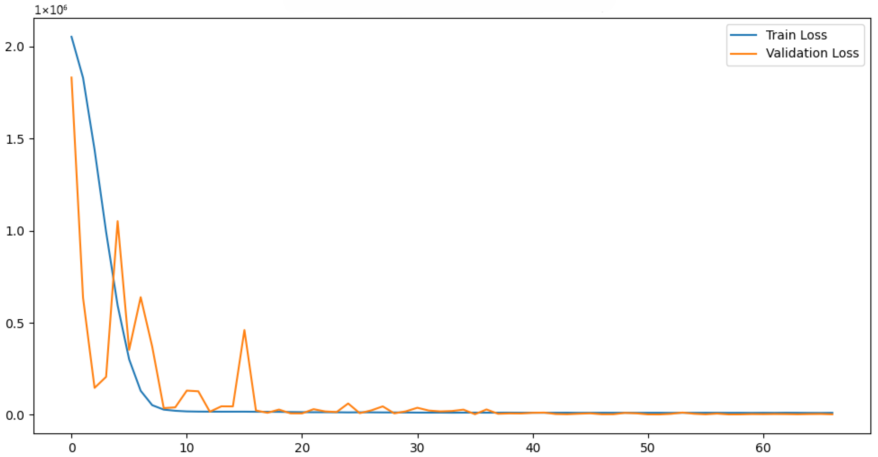
Figure 2 illustrates the baseline convergence behavior of a neural network trained without an explicit temporal input window. The smooth and monotonic decrease in the loss function, without oscillations or divergence, confirms the numerical stability of the optimization process and provides a reference point for subsequent architectures incorporating temporal dependencies. This baseline demonstrates that the learning problem is well-posed and that the chosen optimizer and loss function yield consistent convergence [20].

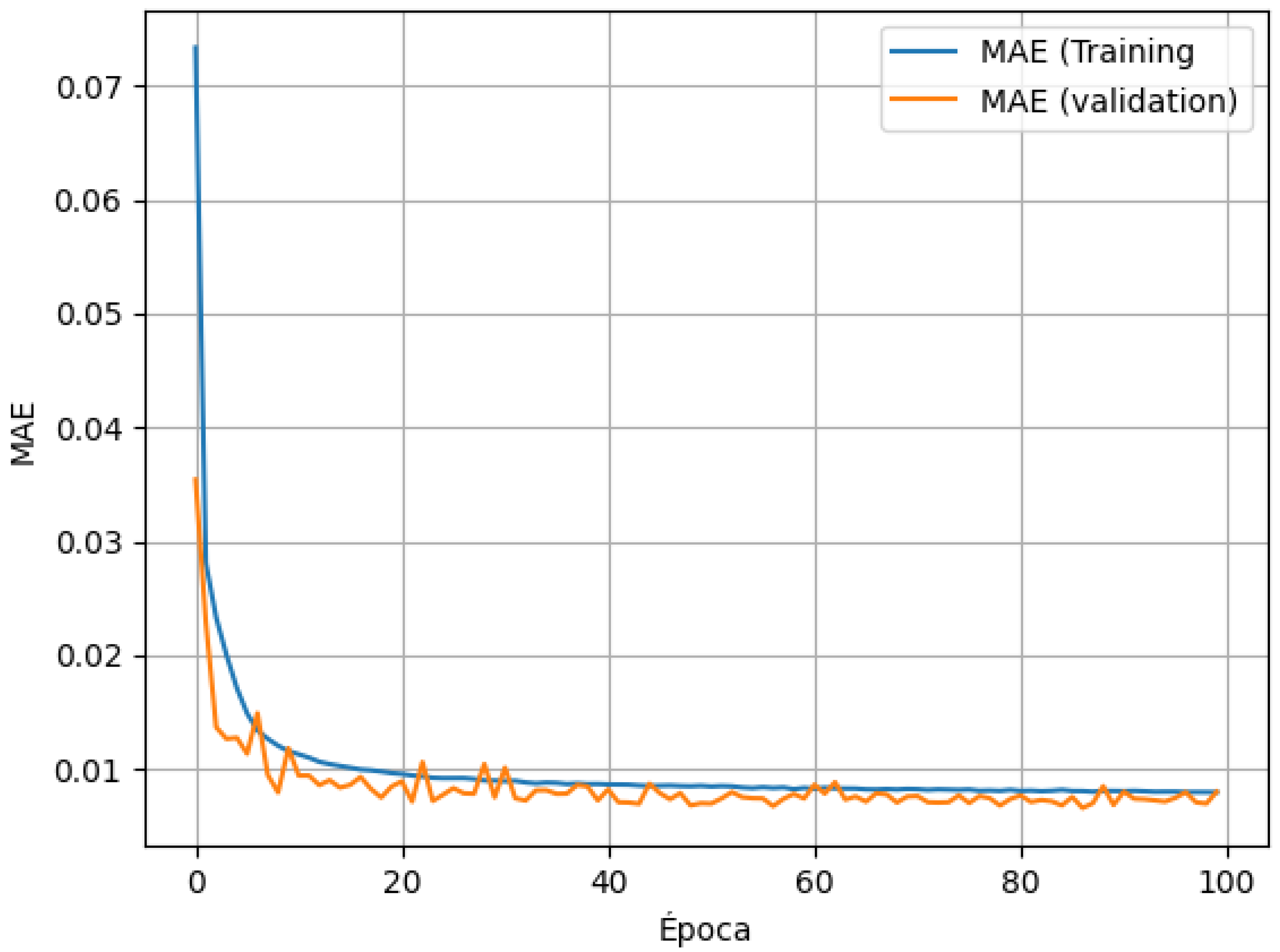
Figure 3 presents the evolution of the validation loss for all evaluated deep learning architectures under the unified training protocol described in Section 2.5. All models exhibited stable convergence, with early stopping effectively preventing overfitting. Differences among architectures were primarily reflected in convergence speed and final loss magnitude, rather than in unstable or divergent behavior. This observation confirms that the subsequent performance differences are attributable to architectural characteristics rather than training artifacts [21]. While all architectures converged without divergence, the LSTM exhibited comparatively weaker validation performance under the same training protocol, indicating reduced generalization in this high-dimensional setting.

Based on this analysis, all models satisfied the minimum stability requirements for inclusion in the comparative evaluation. No model exhibited pathological training behavior that would invalidate its results.

3.2. Error-Based Performance Metrics

Following convergence validation, predictive accuracy was quantified using deterministic error metrics computed over the independent test period (2020–2025). Errors were aggregated across the entire spatiotemporal domain to obtain representative, large-sample estimates of model performance [22,23].

Table 3. Error-based performance metrics for daily solar potential prediction.

Model	RMSE	MAE	R2	Bias	Error Std.	Max Error
CNN	67.80	59.56	0.812	−5.52	67.58	153.30
RNN	32.32	27.80	0.957	5.83	31.79	64.91
LSTM	122.29	105.39	0.387	−3.79	122.23	229.12
GWO	1038.17	717.30	−43.16	−163.79	1025.17	3737.08
MLP	54.80	46.03	0.877	1.49	54.78	148.16

shows the main error-based metrics: Root Mean Squared Error (RMSE), Mean Absolute Error (MAE), coefficient of determination (R²), and bias. Together, these metrics show the average accuracy, the amount of variance explained, and whether there is consistent overestimation or underestimation. Standard deviation and maximum error were also included to measure the extent of error variation and to highlight the largest errors. MAE is highlighted because it is easy to interpret and serves as the fitness function in the MLP–GWO optimization [24].

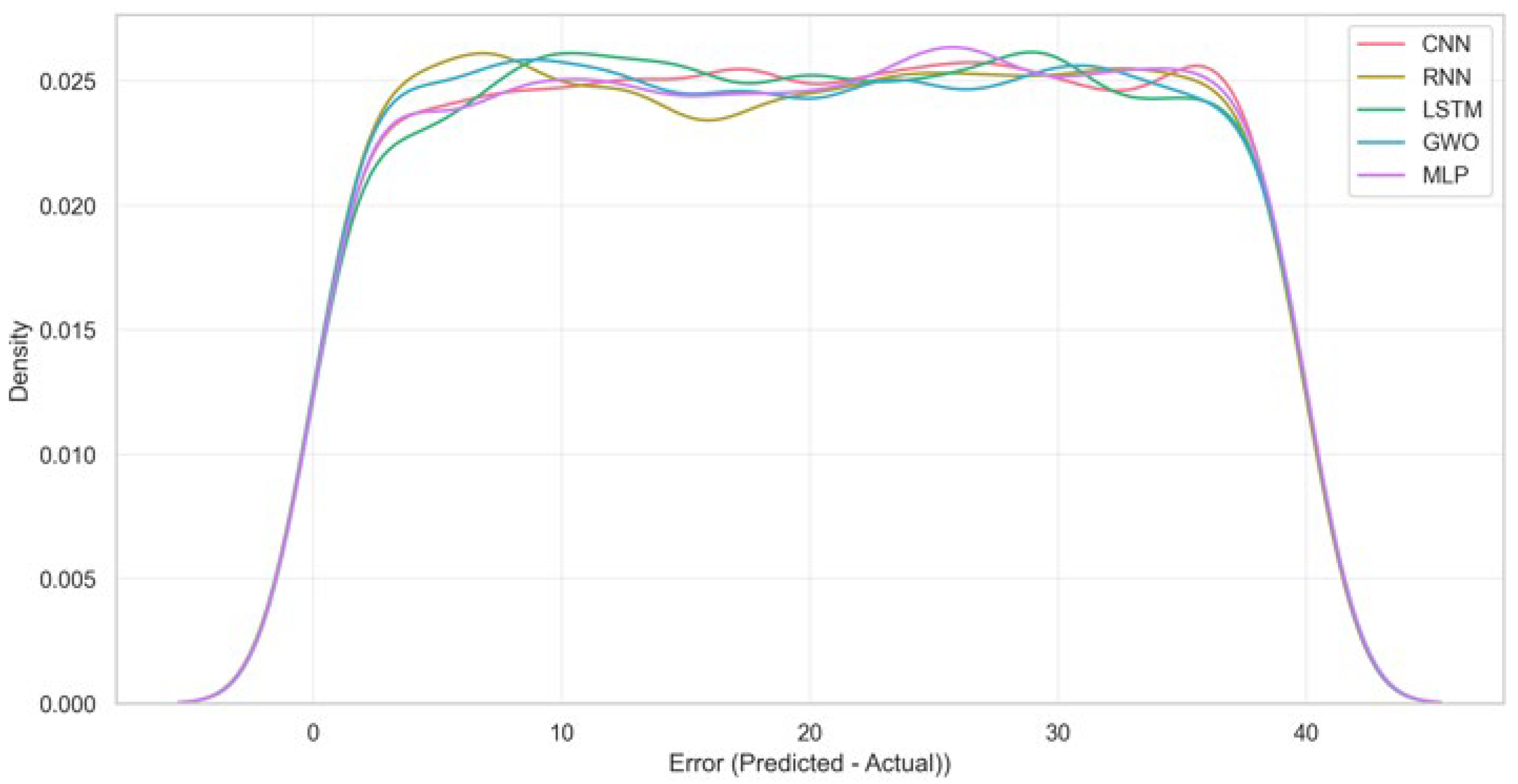
The distribution of prediction errors provides additional insight beyond the mean values. Figure 4 shows the empirical distribution of daily prediction errors for each model. While all architectures produced approximately centered distributions, differences in spread and tail behavior were evident, highlighting the importance of distribution-aware evaluation for solar energy applications [25].

Figure 5 complements the distributional analysis by summarizing the main error-based performance metrics (RMSE, MAE, and bias) for each model, enabling a clear quantitative comparison of overall accuracy and systematic tendencies across architectures.

3.3. Distribution- and Similarity-Based Metrics

To assess how well each model reproduced the full statistical distribution of daily solar potential—including extremes relevant for energy planning—distribution- and similarity-based metrics were computed.

Table 4. Distribution- and similarity-based evaluation metrics for daily solar potential prediction.

Model	P95	Correlation	IOA	JSD	Wasserstein
CNN	114.94	0.986	0.925	5.48 × 10−4	58.64
RNN	56.03	0.9999	0.991	1.13 × 10−4	27.78
LSTM	203.89	0.888	0.599	1.74 × 10−3	101.19
GWO	2421.38	0.152	0.175	∞	601.35
MLP	94.99	0.940	0.969	3.57 × 10−4	18.20

reports the high-percentile errors (P95), correlation, index of agreement (IOA), Jensen–Shannon Divergence (JSD), and the Wasserstein distance between the predicted and reference distributions [26,27]. These metrics complement pointwise error measures by quantifying differences in distribution shape, location, and extreme behavior, where lower values indicate closer agreement with the ERA5-derived reference distribution.

These metrics add to pointwise error measures by showing how similar the distributions are, how they behave at the extremes, and how well the predicted and reference datasets match overall. For divergence and distance measures like Jensen–Shannon and Wasserstein, lower values mean closer agreement. For correlation and agreement metrics, higher values show better performance.

3.4. Statistical Significance Testing

To determine whether observed performance differences between models were statistically meaningful, a non-parametric hypothesis testing framework was applied. The Wilcoxon signed-rank test was conducted on paired daily absolute error series from the test period for each model pair. This test does not assume normality and is well-suited for large, dependent error samples typical of spatiotemporal climate data [28].

A significance level of p < 0.05 was used to reject the null hypothesis of equal median performance. The results confirm that several of the observed differences—particularly between lightweight and more complex architectures—were statistically significant, supporting the robustness of the comparative rankings [29].

3.5. Summary of Validation Findings

Overall, the validation analysis confirms that:

• All models exhibited stable and well-behaved training convergence;
• Predictive differences were not attributable to optimization artifacts or overfitting;
• Error distributions and statistical tests provide consistent evidence for meaningful performance contrasts between architectures.

These findings establish a solid methodological foundation for the subsequent interpretation of results. Accordingly, the next section integrates predictive performance with computational cost considerations to discuss practical trade-offs and implications for resource-constrained solar forecasting applications.

4. Results and Discussion

This section synthesizes the validation outcomes from Section 3 to directly address the research hypotheses (H1, H2) and discuss their practical implications for daily solar potential forecasting under computational constraints. The results are interpreted through the lens of accuracy–efficiency trade-offs, spatial and temporal fidelity, and operational applicability over topographically complex regions using ERA5 data. In this context, the failure of the MLP–GWO model is treated as a structurally meaningful result rather than an anomaly, providing empirical evidence of the limitations of metaheuristic optimization in high-dimensional spatiotemporal regression and reinforcing the continued relevance of gradient-based learning for operational solar forecasting.

4.1. Hypothesis Validation: Accuracy vs. Computational Efficiency Trade-Off

The results show that under the present experimental setting, simpler neural architectures such as MLP and RNN can match or even outperform more complex models such as LSTM and CNN while requiring substantially lower computational resources. Among all of the evaluated models, the RNN achieved the highest predictive accuracy (RMSE ≈ 32.3, MAE ≈ 27.8, R² ≈ 0.96), and the MLP also exhibited competitive performance (R² ≈ 0.88). In contrast, the LSTM and CNN presented higher error levels (R² ≈ 0.39 and 0.81, respectively), despite their greater architectural complexity. The LSTM, in particular, displayed clear signs of overfitting, as illustrated in Figure 3.

The comparatively low performance of the LSTM relative to the simpler RNN, despite both models being trained with the same 30-day input window, suggests sensitivity to training configuration rather than an intrinsic limitation of gated recurrent units. In spatiotemporal regression problems characterized by extremely high-dimensional output spaces (10,965 outputs), LSTM architectures can become more difficult to optimize and are more susceptible to over-parameterization under limited regularization. Although vanishing or exploding gradients were not explicitly diagnosed, the observed training instability and divergence between training and validation errors are consistent with gradient sensitivity issues commonly reported in deep recurrent architectures operating under high-dimensional output constraints.

Within the unified training protocol adopted in this study, the LSTM consistently exhibited poorer validation behavior than the RNN. This outcome is compatible with several non-exclusive factors, including suboptimal learning-rate dynamics, insufficient regularization relative to model capacity, and a potential mismatch between the fixed 30-day temporal window and the effective temporal dependencies governing daily GHI fields. These observations motivate future controlled experiments incorporating gradient clipping, alternative learning-rate schedules, and different look-back windows to assess whether LSTM performance can be recovered under a more carefully tuned regime. Similar behavior has been reported in previous studies, where well-tuned simpler architectures matched or outperformed more complex models in daily forecasting tasks [17,19].

From a computational perspective, both the RNN and MLP achieved their predictive skill with substantially lower training time and GPU memory consumption than the LSTM and the MLP–GWO, as detailed in Section 2.4. This favorable balance between accuracy and efficiency makes these simpler architectures particularly attractive for operational or resource-constrained environments [17,19,30].

Regarding Hypothesis H2, the results indicate that incorporating the Grey Wolf Optimizer (GWO) to tune the MLP did not provide performance gains sufficient to offset the additional computational cost. The MLP–GWO model produced unrealistic predictions, with extremely large errors (RMSE ≈ 1038.2) and a highly negative coefficient of determination (R² ≈ −43.2; Table 3 and Table 4). Quantitatively, while the baseline MLP achieved an RMSE ≈ 54.8, MAE ≈ 46.0, and R² ≈ 0.88, the MLP–GWO configuration yielded an RMSE ≈ 1038.2, MAE ≈ 717.3, and R² ≈ −43.2, together with very large P95 errors (≈ 2421.4 kWh·m⁻²·day⁻¹) and infinite Jensen–Shannon divergence (Table 3 and Table 4). These metrics demonstrate that under the present configuration, the parameter sets selected by the GWO led to predictions that were statistically incompatible with the ERA5-based reference distribution.

It is important to explicitly acknowledge that no dedicated diagnostic analyses of the GWO optimization process were performed in this study. In particular, convergence trajectories, sensitivity to population size, and sensitivity to the number of iterations were not systematically evaluated. The reported results therefore correspond to a representative, but not exhaustive, configuration of the metaheuristic search. For reproducibility, the final GWO-selected setup consisted of 384 and 192 neurons in the first and second hidden layers, respectively, a dropout rate of 0.28, and a learning rate of 4.2 × 10⁻³, with a population of 20 individuals evolved over 30 iterations using validation MAE as the fitness metric.

Under this specific experimental configuration—characterized by an extremely high-dimensional output space (10,965 grid points), spatially aggregated error metrics acting as a noisy fitness signal, and a limited search budget—the use of a population-based, gradient-free optimizer to tune the MLP yielded no practical performance advantages over standard gradient-based training. However, these findings should not be interpreted as a general limitation of the Grey Wolf Optimizer or of metaheuristic optimization methods as a class [5,31], but rather as an outcome that is conditional on the constraints and design choices of the present study.

Regarding temporal context, the recurrent models (RNN and LSTM) were trained using a 30-day input window, whereas the MLP and 1D-CNN relied on single-day inputs, following common practice in daily atmospheric forecasting. Since the LSTM did not outperform the RNN even under identical input-window conditions, the observed performance differences can more plausibly be attributed to differences in model stability and optimization behavior rather than to input length alone. A sensitivity analysis conducted for the RNN using 7-, 15-, and 30-day input windows showed progressively improved performance with increasing window length, which saturated around 30 days, suggesting diminishing returns. This behavior indicates that the RNN’s predictive skill arises from capturing sub-seasonal temporal patterns rather than simply from increased historical input.

Overall, the limitations identified for the MLP–GWO configuration are strictly conditional on the present experimental setup, including the ERA5-driven predictors, the specific MLP architecture summarized in Table 2, and the GWO hyperparameter ranges described in Section 2.5.1. Consequently, while gradient-based optimization remains more reliable and efficient than the tested GWO configuration for this particular high-dimensional daily solar forecasting task, broader conclusions regarding metaheuristic optimization require further targeted investigation beyond the scope of this study.

4.2. Spatial Fidelity: Emulation of ERA5 Patterns and Topographic Limitations

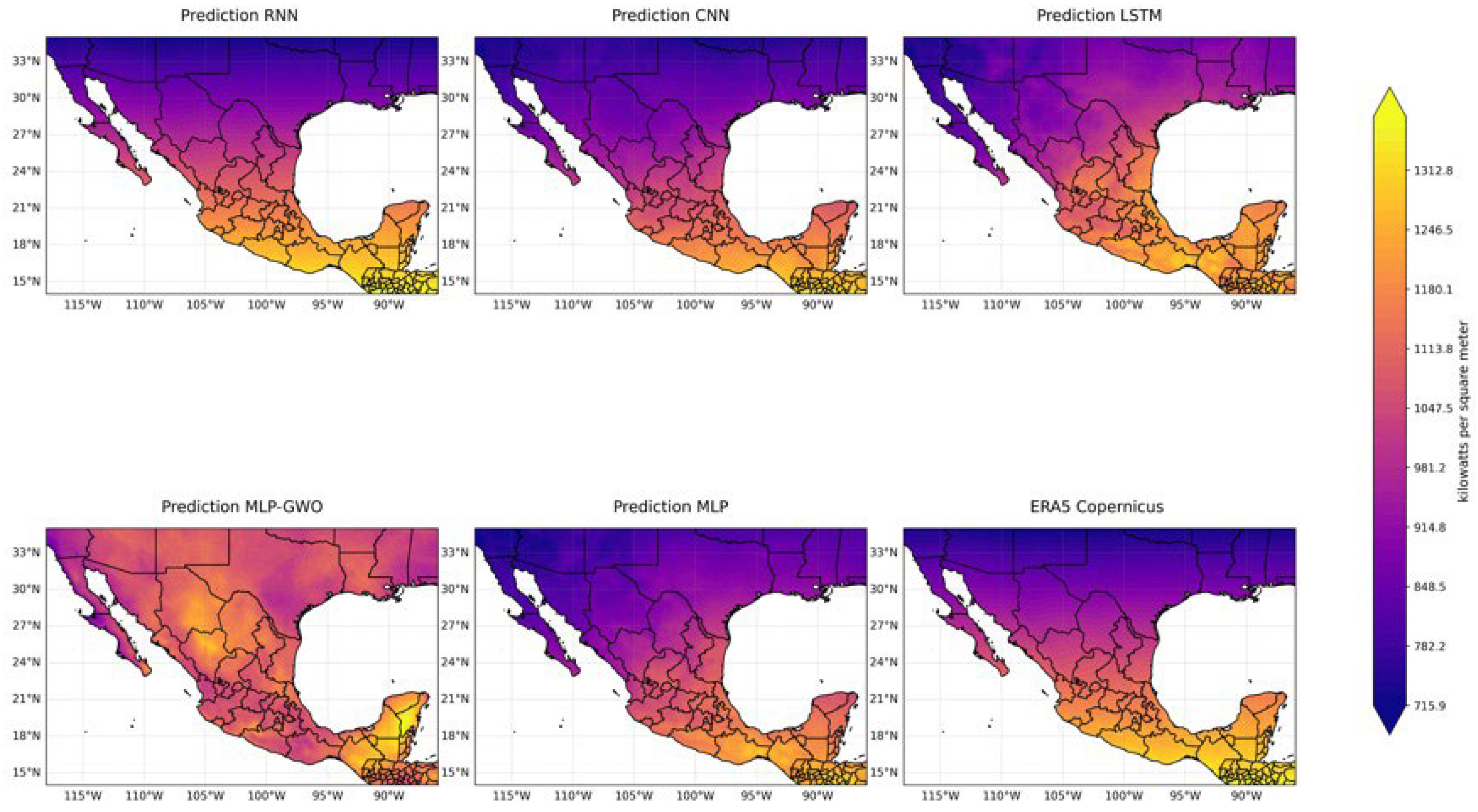
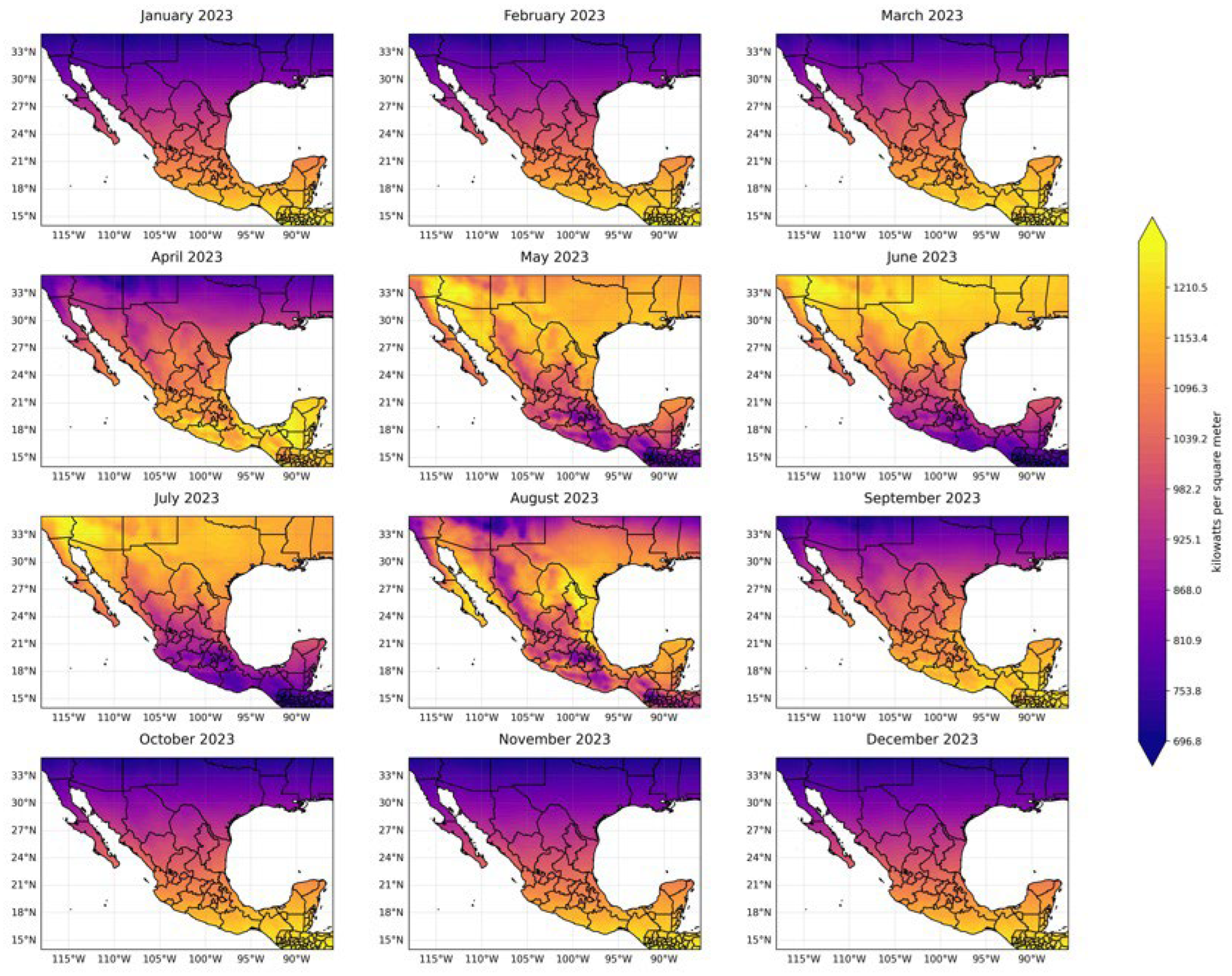
The spatial prediction maps (Figure 6, Figure 7 and Figure 8) complement the statistical evaluation by illustrating how effectively the different models reproduce the large-scale spatial structure of ERA5-based solar potential over Mexico. Rather than aiming at fine-scale spatial downscaling, the evaluated architectures are explicitly designed to function as fast spatial surrogates of ERA5 climatology under constrained computational resources, consistent with the lightweight modeling objective of this study.

• Reproduction of Dominant Spatial Patterns

The RNN and MLP models successfully reconstructed the dominant spatial gradients of daily solar potential across the Mexican domain. These include the high-irradiance plateaus over northern Mexico, reduced values in the more humid southeastern regions, and broad modulations associated with major orographic features such as the Sierra Madre Occidental. This behavior indicates that even relatively lightweight architectures are capable of learning the nonlinear mapping between coarse-scale atmospheric predictors and surface solar radiation fields at the ERA5 spatial scale, including over topographically complex regions [26].

Importantly, the reproduced patterns correspond to the large-scale climatological structure represented in ERA5, rather than to localized fine-scale variability. This is consistent with the intended role of the models as statistical emulators of reanalysis fields rather than as downscaling tools.

• Spatial Error Structure and Inherited ERA5 Limitations

The spatial distribution of prediction errors is structured rather than random. The largest discrepancies relative to ERA5 were concentrated in regions where the reanalysis itself is known to exhibit higher uncertainty, particularly areas characterized by complex terrain and persistent cloud cover, such as southern Mexico and the Gulf of Mexico region [6,9]. This suggests that the models largely inherit the spatial smoothness and limitations of the ERA5 product, rather than correcting its known biases.

The localized noise and artifacts observed in the CNN and LSTM spatial maps (Figure 8) further support this interpretation. These patterns indicate that the networks primarily learn and reproduce the ERA5 spatial climatology at its native ~0.25° resolution, including its smoothing behavior, instead of generating physically sharper gradients or performing implicit statistical downscaling [11].

• Justification and Limitations of the Flattened Spatial Representation

As anticipated in Section 2.5.1, the relatively weaker performance of the 1D-CNN compared to the RNN is largely attributable to the adopted data representation rather than to an intrinsic limitation of convolutional modeling. In this study, the spatial grid was intentionally flattened into a one-dimensional index, thereby removing explicit two-dimensional latitude–longitude neighborhood relationships. This design choice was made to enforce architectural comparability across model families and to keep memory usage and training time within the hardware constraints defined by Hypotheses H1 and H2.

Under this representation, one-dimensional convolutional filters operate along a linearized feature sequence that lacks physical spatial adjacency. As a result, the CNN is inherently constrained in its ability to extract coherent spatial features that depend on local two-dimensional neighborhoods. The noisier and less spatially coherent CNN forecasts observed in regions of complex topography (Figure 8) therefore reflect a loss of spatial topology rather than a fundamental shortcoming of convolutional approaches.

Two-dimensional convolutional architectures that preserve spatial adjacency would be better suited to capturing such features; however, their substantially higher memory and computational requirements place them outside the scope of the proposed lightweight framework and the resource constraints considered in this work.

• Scope and Implications for Lightweight Spatial Modeling

These findings indicate that 1D-CNNs applied to flattened geophysical fields offer limited advantages when strict computational constraints are imposed. While more expressive convolutional architectures may yield improved spatial coherence if spatial structure is preserved and hardware limitations are relaxed, such configurations fell beyond the objectives of this study.

Accordingly, the comparatively weaker and noisier performance of the 1D-CNN should not be interpreted as evidence against convolutional modeling for solar radiation forecasting in general. Instead, it is a direct consequence of the intentionally simplified spatial representation and strict computational constraints adopted here. Under representations that preserve two-dimensional spatial adjacency—such as lightweight 2D CNNs or patch-based convolutional schemes—convolutional architectures would be expected to demonstrate stronger spatial coherence, but at the cost of increased memory usage and training time.

Overall, the proposed models should be interpreted as efficient and statistically consistent emulations of ERA5-based solar potential rather than as high-resolution spatial reconstructions. They are therefore best interpreted as being suitable for applications where ERA5-level accuracy is sufficient, including regional solar resource assessment, preliminary site screening, and system-level energy modeling requiring spatially complete daily inputs [6,32].

4.3. Sub-Regional and Seasonal Error Analysis

To better understand the overall performance, we examined how prediction errors changed by region and season in Mexico. We aimed to find patterns in model performance related to climate zones and seasonal weather, rather than provide detailed local validation.

• Sub-regional Error Patterns

We divided Mexico into broad regions based on climate and terrain: northern arid areas, the central highlands with complex terrain, and southern humid regions. All models had the lowest errors in northern Mexico, where clear skies are common. In the central and southern regions, errors were higher, likely due to complex terrain, frequent clouds, and more uncertainty in ERA5 surface radiation estimates [6,9]. The RNN and MLP models performed steadily across regions, while the 1D-CNN model showed more performance loss in complex terrain.

• Seasonal Error Variability

When we compared different seasons, we saw that the prediction errors changed with the weather. Errors were lowest during the dry season (DJF–MAM), when large-scale weather patterns, which ERA5 models well, control solar radiation. In the summer rainy season (JJA), all models had higher errors due to more clouds and greater small-scale weather changes. Despite these seasonal shifts, the RNN and MLP models still outperformed the more complex models.

In summary, these results show that lightweight models perform well across different regions and seasons, although they still have ERA5’s known limits in areas and times with many small-scale weather changes. This suggests that they constitute a viable option for regional studies where efficiency and broad coverage are prioritized over fine-scale local accuracy, where efficiency and broad coverage are more important than very detailed local accuracy [6,32].

4.4. Evaluation Against Ground-Based Radiometric Stations (CONAGUA/SMN)

To evaluate predictive skill beyond the ERA5 benchmark, we used available ground-based daily global horizontal irradiance (GHI) observations from stations operated by the Mexican National Meteorological Service (SMN–CONAGUA) over the 2020–2025 test period. These observations provide an independent, real-world reference for assessing the absolute performance of the proposed surrogate models.

We compared five surrogate models (MLP, RNN, LSTM, 1D-CNN, and MLP–GWO). For each station and day, model predictions were extracted from the nearest ERA5 grid cell (0.25° × 0.25°), and daily absolute errors were computed against the corresponding observed daily GHI values. No spatial interpolation or statistical bias correction was applied. Accordingly, this evaluation does not aim to correct systematic ERA5 biases, but rather to provide an indicative assessment of model skill under realistic observational constraints.

This comparison inherently involves a scale mismatch between point-based measurements and grid-cell average estimates. Previous studies have shown that such representativeness differences introduce unavoidable discrepancies, particularly in regions characterized by complex topography, coastal transitions, and convective cloud regimes. Consequently, the station-based evaluation should be interpreted as a broad indicator of real-world performance rather than a strict point-scale validation.

Across the SMN–CONAGUA stations, the RNN and MLP models exhibited the lowest errors and minimal bias, consistent with their strong performance in the ERA5-based validation. The LSTM model showed comparable but slightly weaker performance. The 1D-CNN yielded higher errors, likely reflecting its inability to preserve two-dimensional spatial relationships when operating on flattened spatial fields. The MLP–GWO model performed substantially worse, indicating that its metaheuristic optimization strategy does not generalize well when confronted with observational data.

Despite these limitations, the results indicate that the proposed lightweight models preserve strong daily temporal coherence and achieve error levels comparable to those reported in previous ERA5–station validation studies in the literature [33]. This supports their potential applicability in practical contexts such as regional solar resource assessment, preliminary site screening, and system-level energy modeling, where ERA5-level accuracy is generally sufficient (

Table 5. Station-based evaluation of daily solar potential predictions against CONAGUA/SMN ground-based GHI observations (2020–2025).

Model	RMSE	MAE	Bias
MLP	1.07	0.80	−0.05
RNN	0.93	0.67	−0.03
LSTM	0.96	0.70	−0.04
1D-CNN	1.21	0.91	−0.10
MLP–GWO	2.48	1.95	−0.33

Note: Metrics correspond to an indicative station-based evaluation using daily GHI observations from SMN–CONAGUA stations. Model outputs were sampled from the nearest ERA5 grid cell without interpolation. Errors reflect both model uncertainty and the known representativeness mismatch between point observations and grid-cell averages. Values are reported to contextualize real-world performance rather than to imply point-scale bias correction. All units are in kWh·m⁻²·day⁻¹.

).

4.5. Integration of the Proposed Forecasting Framework into Microgrid Energy Management Systems

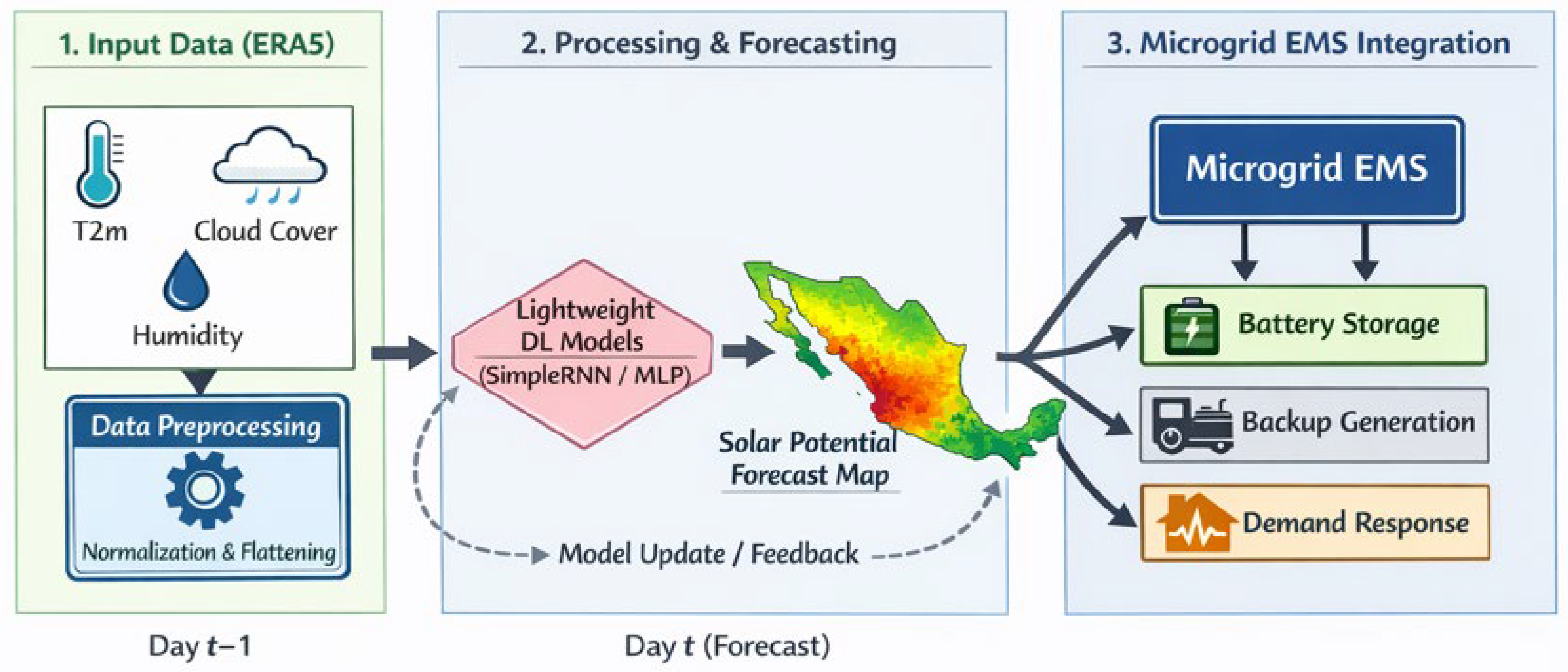
The temporal analysis (confirmed by the high correlation coefficients in Table 4 for RNN and MLP) demonstrates that these models reliably capture the daily and seasonal evolution of solar radiation. Beyond statistical performance, the practical utility of these lightweight surrogates lies in their integration into operational decision-making loops. Figure 9 presents a conceptual day-ahead workflow describing how ERA5 predictors from day t − 1 are ingested by the trained lightweight model (RNN/MLP) to produce a daily solar potential forecast map for day t, which can be integrated into a microgrid energy management system (EMS). In this framework, the resulting forecast can be directly ingested by the EMS to support operational decisions such as battery charge–discharge scheduling, diesel generator dispatch, and load prioritization. For example, in a rural microgrid located in the state of Zacatecas, the daily solar forecast can be used to anticipate periods of reduced photovoltaic generation due to cloud cover, allowing the EMS to pre-charge batteries or schedule auxiliary generation in advance. Conversely, during high-irradiance days, excess solar energy can be allocated to storage or flexible loads. While the temporal resolution is daily, the key operational advantage lies in the inference speed. Once trained, generating a forecast for the next day over the entire country is a matter of seconds on modest hardware, requiring only the previous day’s predictor data. This is vastly more efficient than running a full physical model or performing extensive real-time data processing from the Copernicus API. This efficiency enables rapid scenario analysis and integration into time-sensitive decision loops, particularly in resource-constrained microgrids where computational efficiency, robustness, and ease of integration are critical. Rather than replacing existing EMS logic, the proposed framework complements current control strategies by providing reliable and computationally inexpensive solar forecasts that enhance operational resilience [34].

4.6. Consistency with ERA5 and Implications for Fast Surrogate Modeling

In summary, the findings of this study support a practical and context-specific approach for deploying lightweight neural network models as fast and computationally efficient surrogates of ERA5-derived daily solar potential, under constrained hardware and operational conditions. Rather than aiming to replace physical reanalysis systems, the proposed framework provides a statistically consistent emulation of ERA5 solar potential fields at the native spatial and temporal scales resolved by the reanalysis, enabling accessible energy analytics within clearly defined computational and methodological limits.

1.

Model Selection and Training (Offline Phase).

Within the specific experimental configuration evaluated in this study—namely daily-resolution forecasting driven exclusively by ERA5 predictors and trained under the hardware constraints described in Section 2.4—the results indicate that an RNN offers the most favorable balance between predictive accuracy, convergence stability, and computational cost. An MLP represents a viable alternative when simplicity and minimal training overhead are prioritized. In both cases, the models are trained once using long-term ERA5 data on affordable consumer-grade hardware, after which no further retraining is required for routine deployment.

2.

Integration and Deployment (Operational Phase).

Once trained, the selected model can be deployed as a lightweight, standalone forecasting module. Its inputs consist of preprocessed meteorological variables from the previous day (t − 1), obtained either from ERA5 near-real-time products or from regional numerical weather prediction outputs with comparable structure. The model output is a complete spatial map of predicted daily solar potential Ps(t) for day t, expressed on the ERA5 grid and fully consistent with its spatial resolution.

3.

Application in Energy Management Systems.

The resulting daily solar potential maps can be integrated into existing energy analysis workflows in several ways, including:

(a)

As inputs to photovoltaic performance simulation tools for estimating the expected generation from existing or planned installations;

(b)

As data layers for Smart Microgrid Energy Management Systems (EMSs) [3,34], supporting day-ahead scheduling of storage systems and dispatchable generation—core functions of intelligent energy systems [27].

In all cases, the forecasts should be interpreted as ERA5-consistent inputs intended for planning and operational screening rather than as high-fidelity ground-truth estimates.

4.

Practical Deployment and Sustainability Considerations.

(a)

Accessibility and operational resilience: By substantially reducing computational requirements, the proposed framework demonstrates a pathway to enable advanced solar forecasting capabilities in regions where high-performance computing resources are unavailable. This potential enhances access to spatially complete solar potential information for local planners and energy operators, particularly in emerging economies [35].

(b)

Computational and environmental efficiency: The use of lightweight models trained once and executed efficiently reduces long-term computational and energy costs relative to continuous high-resolution simulations or large deep learning architectures. This represents a step toward more sustainable data-driven practices in energy and climate analytics, by prioritizing computational efficiency [34,35].

(c)

Scope and limitations: The proposed framework is designed to support—rather than replace—human decision-making. It accelerates the generation of daily, ERA5-consistent solar potential estimates over large areas and integrates naturally into existing planning pipelines. Its primary objective is to provide affordable, scalable decision support at the reanalysis scale, rather than localized bias correction, statistical downscaling, or real-time control [25,36,37].

5.

Synthesis.

Taken together, the results demonstrate that within the specific ERA5-based, daily-resolution, and resource-constrained experimental framework considered in this study, lightweight neural models—particularly RNNs and MLPs—can function as efficient and statistically consistent surrogates of ERA5-derived daily solar potential fields. This consistency holds at the spatial and temporal scales resolved by the reanalysis itself, including regions of complex topography, where the models primarily reproduce large-scale ERA5 climatological patterns rather than correcting known reanalysis uncertainties. Consequently, the results suggest that these models are well-suited for large-scale, preliminary energy planning applications where ERA5-level spatial fidelity is sufficient and computational efficiency is a primary constraint [38].

5. Conclusions

This study systematically evaluated the accuracy–efficiency trade-off of five deep learning architectures for generating daily solar potential maps from ERA5 reanalysis data over Mexico’s complex terrain. The objective was not to maximize predictive skill at all costs, but to assess whether lightweight neural models can provide reliable spatial surrogates under constrained computational resources.

Within this explicitly defined experimental framework—ERA5-based predictors at daily resolution, flattened spatial outputs (10,965 grid points), and the hardware and training constraints described in Section 2.4 and Section 2.5—the results support three principal conclusions that directly address the initial research hypotheses and delimit the scope of the contribution.

Architectural efficiency outweighs unnecessary complexity under constrained conditions.

For the specific task considered here, simpler architectures consistently provided a more favorable balance between predictive accuracy, training stability, and computational cost than more complex alternatives. Under identical input–output representations and training protocols, the RNN achieved the best overall performance (RMSE ≈ 32.3, R² ≈ 0.96), combining high accuracy with stable convergence behavior. The MLP offered a computationally efficient baseline with competitive skill. In contrast, neither the LSTM nor the 1D-CNN yielded systematic performance gains within this setup, and the MLP–GWO configuration failed to converge toward meaningful solutions. These outcomes support Hypotheses H1 and H2 within the tested configuration space, indicating that, under strict resource constraints and high-dimensional outputs, increased architectural sophistication does not necessarily translate into improved performance.

The proposed models function as efficient ERA5-scale surrogates rather than high-fidelity correction tools.

The best-performing models reproduce the dominant large-scale spatial and temporal patterns of ERA5 solar potential, including latitudinal gradients and broad topographic modulation. However, they also inherit the intrinsic characteristics and limitations of the underlying reanalysis, such as spatial smoothing and known uncertainties over complex terrain. Consequently, the framework is best interpreted as a fast and statistically consistent emulator of ERA5 fields, suitable for regional resource assessment and operational planning at the native reanalysis scale. It is not intended for statistical downscaling, bias correction, or sub-daily nowcasting.

A lightweight framework for accessible solar energy analytics.

By prioritizing computational efficiency and architectural parsimony, this work demonstrates a practical pathway for transforming global reanalysis products into usable daily solar forecasting tools without reliance on high-performance computing infrastructure. Within the constraints of the present setup, the framework lowers hardware and operational barriers, making data-driven solar resource assessment more accessible to institutions operating in resource-limited environments. This contributes to more inclusive and scalable energy planning, particularly in emerging economies.

Limitations and future work.

The present study has intentional limitations that define clear directions for further research. First, the achievable fidelity is ultimately bounded by ERA5 itself. Integration with ground-based radiometric observations is a necessary next step to quantify absolute errors and enable bias-aware modeling. Second, the flattened spatial representation constrains the ability of models—particularly convolutional architectures—to exploit spatial adjacency. Future work may explore inherently spatial yet computationally efficient alternatives, such as lightweight graph-based models or attention mechanisms, while explicitly quantifying the associated computational trade-offs. Finally, the practical value of the framework will be fully realized through integration into operational energy management systems, where daily solar forecasts can be directly coupled with photovoltaic performance models and storage optimization to support automated, intelligent grid operation.

In summary, under the present ERA5-driven, daily-resolution experimental design and hardware constraints, the results demonstrate that accurate and spatially explicit solar resource assessment for planning purposes does not require highly complex neural architectures. Within this clearly defined context, the proposed lightweight framework offers a robust and accessible bridge between large-scale climate reanalysis data and practical solar energy applications in regions where computational infrastructure remains limited.

References

1. Voyant, C.; Muselli, M.; Paoli, C.; Nivet, M.-L. Machine learning methods for solar radiation forecasting: A review. Renew. Energy 2017, 105, 569–582. [Google Scholar] [CrossRef]
2. Shi, X.; Chen, Z.; Wang, H.; Yeung, D.-Y.; Wong, W.-K.; Woo, W.-C. Convolutional LSTM network: A machine learning approach for precipitation nowcasting. Adv. Neural Inf. Process. Syst. 2015, 28. Available online: https://proceedings.neurips.cc/paper/2015/hash/07563a3fe3bbe7e3ba84431ad9d055af-Abstract.html (accessed on 15 July 2025).
3. Abdel-Nasser, M.; Mahmoud, K. Accurate photovoltaic power forecasting models using deep LSTM–RNN. Neural Comput. Appl. 2019, 31, 2727–2740. [Google Scholar] [CrossRef]
4. Bacher, P.; Madsen, H.; Nielsen, H.A. Online short-term solar power forecasting. Sol. Energy 2009, 83, 1772–1783. [Google Scholar] [CrossRef]
5. Mirjalili, S. How effective is the Grey Wolf optimizer in training multi-layer perceptrons. Appl. Intell. 2015, 43, 150–161. [Google Scholar] [CrossRef]
6. Sawadogo, W.; Reboita, M.S.; Faye, A.; da Rocha, R.P.; Odoulami, R.C.; Olusegun, C.F.; Adeniyi, M.O.; Abiodun, B.J.; Sylla, M.B.; Diallo, I.; et al. Current and future potential of solar and wind energy over Africa using the RegCM4 CORDEX-CORE ensemble. Clim. Dyn. 2021, 57, 1647–1672. [Google Scholar] [CrossRef]
7. Hans, C.A.; Klages, E. Very Short Term Time-Series Forecasting of Solar Irradiance Without Exogenous Inputs. arXiv 2018, arXiv:1810.07066. [Google Scholar] [CrossRef]
8. Hersbach, H.; Bell, B.; Berrisford, P.; Biavati, G.; Horányi, A.; Muñoz Sabater, J.; Nicolas, J.; Peubey, C.; Radu, R.; Rozum, I.; et al. ERA5 hourly data on single levels from 1940 to present. Copernic. Clim. Change Serv. (C3S) Clim. Data Store (CDS) 2023. [Google Scholar] [CrossRef]
9. Boussif, O.; Boukachab, G.; Assouline, D.; Massaroli, S.; Yuan, T.; Benabbou, L.; Bengio, Y. Improving day-ahead solar irradiance time series forecasting by leveraging spatio-temporal context. arXiv 2023, arXiv:2306.01112. [Google Scholar] [CrossRef]
10. Khan, S.; Mazhar, T.; Khan, M.A.; Shahzad, T.; Ahmad, W.; Bibi, A.; Saeed, M.M.; Hamam, H. Comparative analysis of deep neural network architectures for renewable energy forecasting: Enhancing accuracy with meteorological and time-based features. Discover. Sustain. 2024, 5, 533. [Google Scholar] [CrossRef]
11. Assaf, A.M.; Haron, H.; Hamed, H.N.A.; Ghaleb, F.A.; Qasem, S.N.; Albarrak, A.M. A review on neural network based models for short-term solar irradiance forecasting. Appl. Sci. 2023, 13, 8332. [Google Scholar] [CrossRef]
12. Shao, X.; Lu, S.; Hamann, H.F. Solar radiation forecast with machine learning. In Proceedings of the AM-FPD; Kyoto, Japan, 6–8 July 2016, IEEE: New York, NY, USA, 2016; pp. 19–22. [Google Scholar] [CrossRef]
13. Alzahrani, A.; Shamsi, P.; Ferdowsi, M.; Dagli, C. Solar irradiance forecasting using deep recurrent neural networks. In Proceedings of the ICRERA, San Diego, CA, USA, 5–8 November 2017; IEEE: New York, NY, USA, 2017; pp. 988–994. [Google Scholar] [CrossRef]
14. Gensler, A.; Henze, J.; Sick, B.; Raabe, N. Deep Learning for solar power forecasting—An approach using AutoEncoder and LSTM Neural Networks. In Proceedings of the 2016 IEEE International Conference on Systems, Man, and Cybernetics (SMC), Budapest, Hungary, 9–12 October 2016; IEEE: New York, NY, USA, 2016; pp. 002858–002865. [Google Scholar] [CrossRef]
15. Paxi-Apaza, W.; Clares-Perca, J.; Flores, A. Solar radiation prediction with deep learning and data augmentation. In Proceedings of the IEEE SEST, Lima, Peru, 5–7 August 2021. [Google Scholar] [CrossRef]
16. Marzouq, M.; El Fadili, H.; Lakhliai, Z.; Zenkouar, K. A review of solar radiation prediction using artificial neural networks. In Proceedings of the 2017 International Conference on Wireless Technologies, Embedded and Intelligent Systems (WITS), Fez, Morocco, 19–20 April 2017; IEEE: New York, NY, USA, 2017; pp. 1–6. [Google Scholar] [CrossRef]
17. Pang, Z.; Niu, F.; O’Neill, Z. Solar radiation prediction using recurrent neural network and artificial neural network. Renew. Energy 2020, 156, 279–289. [Google Scholar] [CrossRef]
18. Hossain, M.S.; Mahmood, H. Short-term photovoltaic power forecasting using an LSTM neural network. IEEE Access 2020, 8, 172524–172533. [Google Scholar] [CrossRef]
19. Azizi, N.; Yaghoubirad, M.; Farajollahi, M.; Ahmadi, A. Deep learning-based long-term global solar irradiance forecasting using time series with multi-step multivariate output. Renew. Energy 2023, 206, 135–147. [Google Scholar] [CrossRef]
20. Ağbulut, Ü.; Gürel, A.E.; Biçen, Y. Prediction of daily global solar radiation using different machine learning algorithms: Evaluation and comparison. Renew. Sustain. Energy Rev. 2021, 135, 110114. [Google Scholar] [CrossRef]
21. Feng, Y.; Gong, D.; Zhang, Q.; Jiang, S.; Zhao, L.; Cui, N. Evaluation of temperature-based machine learning and empirical models for predicting daily global solar radiation. Energy Convers. Manag. 2019, 198, 111780. [Google Scholar] [CrossRef]
22. Jiao, X.; Li, X.; Lin, D.; Xiao, W. Graph Neural Network Based Deep Learning Predictor for Spatio-Temporal Group Solar Irradiance Forecasting. IEEE Trans. Ind. Inform. 2022, 18, 6142–6149. [Google Scholar] [CrossRef]
23. Tajjour, S.; Chandel, S.S.; Alotaibi, M.A.; Malik, H.; Márquez, F.P.G.; Afthanorhan, A. Short-term solar irradiance forecasting using deep learning techniques: A comprehensive case study. IEEE Access 2023, 11, 119851–119861. [Google Scholar] [CrossRef]
24. Ladjal, B.; Nadour, M.; Bechouat, M.; Hadroug, N.; Sedraoui, M.; Rabehi, A.; Guermoui, M.; Agajie, T.F. Hybrid deep learning CNN–LSTM model for forecasting direct normal irradiance: A study on solar potential in Ghardaia, Algeria. Sci. Rep. 2025, 15, 15404. [Google Scholar] [CrossRef] [PubMed]
25. Alkhayat, G.; Mehmood, R. A review and taxonomy of wind and solar energy forecasting. Energy AI 2021, 4, 100060. [Google Scholar] [CrossRef]
26. Krishnan, N.; Kumar, K.R.; Inda, C.S. How solar radiation forecasting impacts the utilization of solar energy: A critical review. J. Clean. Prod. 2023, 388, 135860. [Google Scholar] [CrossRef]
27. Alzahrani, A.; Shamsi, P.; Dagli, C.; Ferdowsi, M. Solar Irradiance Forecasting Using Deep Neural Networks. Procedia Comput. Sci. 2017, 114, 304–313. [Google Scholar] [CrossRef]
28. Khosravi, A.; Nahavandi, S.; Creighton, D.; Atiya, A.F. Comprehensive review of neural network-based prediction intervals and new advances. IEEE Trans. Neural Netw. 2011, 22, 1341–1356. [Google Scholar] [CrossRef]
29. Merizzi, F.; Asperti, A.; Colamonaco, S. Wind speed super-resolution and validation: From ERA5 to CERRA via diffusion models. Neural Comput. Applic. 2024, 36, 21899–21921. [Google Scholar] [CrossRef]
30. Vaswani, A.; Shazeer, N.; Parmar, N.; Uszkoreit, J.; Jones, L.; Gomez, A.N.; Kaiser, Ł.; Polosukhin, I. Attention is all you need. Adv. Neural Inf. Process. Syst. 2017, 30, 15. [Google Scholar] [CrossRef]
31. Faramarzi, A.; Heidarinejad, M.; Stephens, B.; Mirjalili, S. Equilibrium optimizer: A novel optimization algorithm. Knowl.-Based Syst. 2020, 191, 105190. [Google Scholar] [CrossRef]
32. Heidari, A.A.; Mirjalili, S.; Faris, H.; Aljarah, I.; Mafarja, M.; Chen, H. Harris hawks optimization: Algorithm and applications. Future Gener. Comput. Syst. 2019, 97, 849–872. [Google Scholar] [CrossRef]
33. Hersbach, H.; Bell, B.; Berrisford, P.; Hirahara, S.; Horányi, A.; Muñoz-Sabater, J.; Nicolas, J.; Peubey, C.; Radu, R.; Schepers, D.; et al. The ERA5 global reanalysis. Q. J. R. Meteorol. Soc. 2020, 146, 1999–2049. [Google Scholar] [CrossRef]
34. European Commission. Industry 5.0: Towards a Sustainable, Human-Centric and Resilient European Industry; Publications Office of the European Union: Luxembourg, 2021. [Google Scholar] [CrossRef]
35. Green AI Institute. White Paper on the Global Environmental Impact of Artificial Intelligence; Technical Report; Green AI Institute: Boston, MA, USA, 2025; Available online: https://www.greenai.institute/whitepaper/white-paper-on-global-artificial-intelligence-environmental-impact (accessed on 15 November 2025).
36. Instituto Nacional de Estadística y Geografía (INEGI). Atlas de Radiación Solar de México; INEGI: Aguascalientes, Mexico, 2018. [Google Scholar]
37. Guevara, M.; Taufer, M.; Vargas, R. Gap-free global annual soil moisture: 15 km grids for 1991–2018. Earth Syst. Sci. Data Discuss. 2020, 13, 1711–1735. [Google Scholar] [CrossRef]
38. Zewe, A. Explained: Generative AI’s Environmental Impact. MIT News, 2025. Available online: https://news.mit.edu/2025/explained-generative-ai-environmental-impact-0117 (accessed on 16 January 2025).
Figure 1. Spatial domain of the study corresponding to the Mexican Republic, delimited between 14° N–35° N and 118° W–86° W (above sea level).
Technologies 14 00097 g001
Figure 2. Baseline training convergence of the neural network without a temporal input window.
Technologies 14 00097 g002
Figure 3. Training and validation loss convergence for the evaluated neural network architectures.
Technologies 14 00097 g003
Figure 4. Distribution of prediction errors for the evaluated models.
Technologies 14 00097 g004
Figure 5. Comparison of RMSE, MAE, and bias across evaluated models.
Technologies 14 00097 g005
Figure 6. Spatial distribution of daily solar potential over Mexico for January 2025, predicted by the RNN model using ERA5-driven inputs. Values correspond to daily global horizontal irradiance (kWh·m−2·day−1) on the native ERA5 grid.
Technologies 14 00097 g006
Figure 7. Comparative visualization of neural network architectures illustrating differences in predictive accuracy and computational cost, based on ERA5-driven daily solar potential forecasting over Mexico.
Technologies 14 00097 g007
Figure 8. Additional spatial prediction maps for different neural network models and representative dates, illustrating differences in spatial coherence and noise when emulating ERA5-derived daily solar potential fields.
Technologies 14 00097 g008
Figure 9. Conceptual workflow for integrating ERA5-driven day-ahead solar potential forecasts into a microgrid energy management system (EMS). ERA5 predictors from day t − 1 are preprocessed and ingested by the trained lightweight model (RNN/MLP) to generate a daily solar potential forecast map for day t, which is then used by the EMS for battery scheduling, backup generation dispatch, and demand response planning.
Technologies 14 00097 g009