Abstract
This paper presents a novel post hoc error correction method that enables deep neural networks to recognize classes that were completely excluded during training. Unlike traditional approaches requiring full model retraining, our method uses hidden layer representations from any pre-trained classifier to detect and correct errors on missing categories. We demonstrate the approach on facial emotion recognition using the RAF-DB dataset, systematically excluding each of the seven emotion classes from training. The results show correction gains of up to 0.811 for excluded classes while maintaining 99% retention on known classes in the best setup. The method provides a computationally efficient alternative to retraining when new categories emerge after deployment.
1. Introduction
Accurate facial emotion recognition has become a cornerstone of the broader domain of affective computing, which aims to develop systems capable of recognizing, interpreting, and responding to human emotions through computational methods [1,2,3]. However, a persistent challenge in facial expression classification is the presence of imbalanced class distributions, where certain emotions are significantly underrepresented [4,5]. Class imbalance often degrades model generalization, leading to biased predictions toward majority classes and poorer recognition of subtle or rare emotions such as fear or disgust [6].
To address such imbalances, researchers have proposed several strategies. Resampling techniques—such as oversampling minority classes or undersampling majority classes—are commonly employed to rebalance datasets, though they risk introducing redundancy or discarding critical information [7,8]. Another approach involves loss reweighting, where algorithms adjust the learning process by assigning greater weight to underrepresented classes. Methods such as class-balanced loss, focal loss, and label-distribution-aware margins exemplify this strategy [9,10,11]. Hybrid approaches combining reweighting and resampling have also been shown to improve robustness in imbalanced emotion datasets [12].
Deep neural networks enhanced with attention mechanisms have demonstrated considerable promise in emotion recognition tasks. For instance, models integrating attention within CNN–LSTM architectures enable the system to focus on discriminative facial regions, thereby improving performance [13,14,15,16]. Furthermore, attention-based frameworks have been explicitly applied to handle uncertainty and class imbalance by emphasizing learning from underrepresented samples [17,18]. Self-attention and Transformer-based architectures have also gained traction, often outperforming traditional CNN-based approaches in scenarios involving noisy or imbalanced data [19,20].
Alongside these developments, a complementary line of research emphasizes AI error correction without retraining legacy systems. This paradigm, pioneered by Gorban and colleagues, introduces external correctors—lightweight modules that detect risky cases and propose alternative decisions. The theoretical foundation rests on stochastic separation theorems, which demonstrate that in high-dimensional spaces, even simple classifiers (such as Fisher’s linear discriminants) can separate error cases from correctly classified ones with high probability [21]. This leads to practical one-shot correction methods capable of improving system reliability without iterative retraining [22,23]. More recent advances generalize these results to fine-grained, clustered data distributions, showing that families of multi-correctors can handle complex structures and even facilitate new class discovery in high-dimensional settings [24,25]. These methods have been validated on benchmarks such as CIFAR-10, where external correctors successfully amended errors of deep convolutional networks and supported incremental learning of novel object classes.
Despite these advances, most studies focus on models trained directly on the full emotion set—with balanced or rebalanced inputs—rather than exploring error correction strategies that recover missing or excluded classes. The present study addresses this gap using an LSTM-based model with an attention mechanism, trained on subsets of emotion classes, followed by error correction applied to the omitted (seventh) class.
In the experiments, the model is trained on all possible combinations of six out of seven emotion classes and then evaluated on its ability to correct predictions for the held-out class. The results show that while the success rate of correction varies across classes, even small or rare emotions benefit, with key metrics—such as precision and recall—improving for minority classes. These findings align with recent evidence suggesting that auxiliary learning and reconstruction-based strategies can significantly enhance minority class recognition in affective computing tasks [26,27].
Recent advances in handling imbalanced datasets for deep learning have explored various innovative approaches. Data augmentation techniques [28] have proven effective for increasing minority class representation, while generative adversarial networks (GANs) [29] can synthesize realistic samples for underrepresented emotions. Metric learning approaches [30] and contrastive learning [31] have shown promise in learning discriminative features for minority classes. Additionally, curriculum learning strategies [32] and self-supervised pre-training [33] have demonstrated improved performance on imbalanced facial expression datasets. Our work complements these approaches by focusing on post-hoc correction rather than rebalancing during training.
Novelty and Contributions: The main contribution of this work is a post-hoc error correction framework that differs from existing approaches in several key aspects:
- It operates after training, requiring no retraining of the base model.
- It can recover completely missing classes excluded from the original training set.
- It is model-agnostic and can work with any pre-trained classifier architecture.
- It maintains performance on original classes while adding capability to recognize new categories.
This finding is particularly relevant for real-world applications where detecting rare or atypical emotional signals is critical—for example, in anti-fraud systems or security contexts. The demonstrated ability to improve recognition of low-frequency classes underscores the practical value of the proposed method in scenarios requiring robust classification under skewed class distributions.
2. Methodology
This section provides the mathematical formulation of our correction approach. The key insight is that hidden representations of neural networks contain sufficient information to detect and correct errors on missing classes.
2.1. The Corrector Model
Let us consider the problem of multiclass classification in the feature space. Let
The basic classifier is defined by the mapping
which assigns a class label to each point .
In this case, the model additionally induces the display
where is interpreted as an embedding vector obtained during the inference process.
To build a correction mechanism, we introduce the binary mapping
where corresponds to familiar data, and corresponds to unfamiliar (out-of-distribution) data.
Based on this, we define a generalized classifier with correction:
Thus, the h function combines two mechanisms:
- Standard classification by means of f on a set of known classes ;
- Identification of new or missing classes using the g corrector.
This separation makes it possible to formalize the error correction task of a pre-trained system as a combination of the classification task and the task of detecting unknown data. In particular, the proposed approach provides
- Resilience to the appearance of classes that were missing at the learning stage;
- The ability to process unbalanced samples by highlighting “rare” or excluded classes;
- The ability to extend the functionality of the original f classifier to the more general h system.
2.2. Metrics for Evaluating the Quality of a Proofreader
Let us give the test set , where . Let us refer to the predictions of the basic (without correction) model f as , and the predictions of the system with correction h as .
For a fixed class , we assume
Let us introduce a set of indexes of class i samples that have been correctly classified by one system or another:
We also denote the error sets (for class i):
2.3. Basic One-Class Metrics
First-class accuracy (synonyms of the True Positive Rate (TPR) for each class):
Relative and absolute increment are determined as follows:
where is a small regularization for stability at zero base.
Conservation and harm metrics for already correctly classified samples.
The characteristic we are interested in is how the corrector affects samples that have already been correctly classified by f. We introduce the following concepts:
Retention—the proportion of samples of class i that were correctly recognized by f, which remained correctly recognized even after applying the corrector:
Harm—the proportion of i class samples correctly recognized by f that became erroneous after correction:
Correction gain—the proportion of previously misclassified Class i samples that became correct after correction:
2.4. Metrics of “Spillover” and False Positives on Other Classes
To take into account how the corrector affects the incorrect reassignment of the label towards class i, we define
as the proportion of samples from other classes that were classified as class i by the h system (i.e., “false positive for i”). Accordingly, for f,
The false positive percentage change is
2.5. Summary Indicators and Standards
The following aggregates are offered for a summary assessment:
One can also weigh the frequencies of the classes , if desired, to get a “micro” version of the metrics:
2.6. Interpretation of Metrics
- close to 1 means that the corrector does not spoil the already correctly recognized samples of class i.
- demonstrates the share of “collateral damage” for already correct predictions; the lower the value the better.
- shows the corrector’s ability to restore previously erroneous examples of this class.
- indicates an increase in false positive assignments to class i (side effect).
3. Data
For analysis, the RAF-DB (Real-world Affective Faces Database) dataset was selected, containing data on the emotions of people of different ages [34]. This dataset was downloaded from the Kaggle website [35].
Examples of images are shown in Figure 1. The dataset contains 15,339 facial images labeled with basic and composite emotions by 40 independent annotators. The label mapper, which shows the face label and the emotion it encodes, is shown in Table 1. The images are highly diverse in features such as age, gender, ethnicity, head rotation, lighting conditions, and the presence of partial occlusions (e.g., glasses, beard, or self-occlusion). In addition, the images may contain filters and special effects, which makes the dataset particularly suitable for emotion recognition tasks in near-real-world settings.
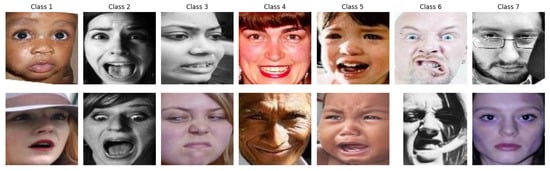
Figure 1.
Examples of images labeled with different emotions in the sample, according to the labels shown in Table 1.

Table 1.
Correspondence between labels and emotions in the RAF-DB dataset (basic emotions).
Distributions of the proportions of classes in each subset are given in Figure 2.
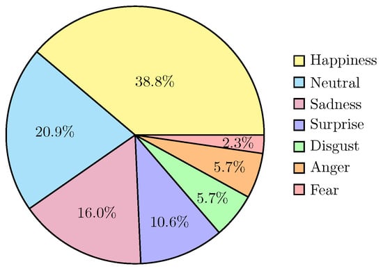
Figure 2.
Pie chart showing the proportion of classes in the initial sample.
4. Proposed Correction Method
Our method consists of two independent components that work in tandem to enable post hoc error correction for missing classes shown in Figure 3.
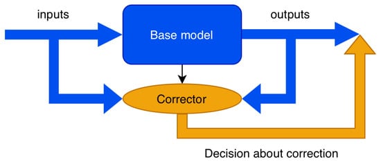
Figure 3.
Principal scheme of correction.
4.1. Base Model
We employ a CNN-LSTM architecture with an attention mechanism for facial emotion recognition. This choice was motivated by our goal to leverage a powerful, state-of-the-art architecture specifically designed for this task. Our implementation is based on the CNN-LSTM facial expression recognition method fused with a two-layer attention mechanism [36], which has demonstrated superior performance.
However, it is crucial to emphasize that any pre-trained classifier can serve as the base model within our framework, highlighting its generalizability. The chosen architecture processes input images through convolutional layers to extract spatial features, which are then reinterpreted as sequential data for the LSTM component. The integrated two-layer attention mechanism dynamically weights the importance of different facial regions across both spatial and temporal dimensions, allowing the model to focus on the most discriminative features for accurate emotion classification.
4.2. Corrector Module
The core innovation of our approach lies in the corrector module, which operates independently of the base model’s architecture:
- Feature Extraction: Collect hidden representations from intermediate layers of the base model, including convolutional feature maps, LSTM hidden states, attention weights, and pre-classification embeddings.
- Corrector Training: Train a gradient boosting classifier (XGBoost) on these extracted features to learn patterns that distinguish between correctly classified samples and potential errors, particularly for classes excluded during base model training.
- Inference Pipeline: During deployment, the corrector analyzes the base model’s hidden representations and can override predictions when it detects high-confidence patterns of excluded classes.
Key Advantage: While we demonstrate the method using CNN-LSTM for emotion recognition, the correction approach is fundamentally model-agnostic. It relies solely on the hidden representations that are available in any deep learning architecture (ResNet, Vision Transformers, etc.), making it applicable across various domains beyond facial emotion recognition.
This separation of concerns allows for the following:
- Computational Efficiency: Lightweight corrector training vs. full model retraining.
- Flexibility: The same correction framework is applicable to different base architectures.
- Incremental Learning: The ability to add new class recognition without modifying deployed models.
- Preservation of Existing Performance: Minimal impact on already learned categories.
The method effectively creates a hybrid system where the base model handles routine classification, while the corrector specializes in identifying and rectifying errors related to previously unseen or underrepresented classes.
5. Technical Implementation of the Experiment
To solve the problem of classifying emotions in facial images, a custom neural network model was developed that combines convolutional layers for feature extraction, a recurrent component (LSTM) for modeling the spatial–sequential structure, and an attention mechanism for identifying the most informative features.
The feature sequence from the convolutional block is processed by an LSTM layer. The LSTM’s role is to model non-linear spatial dependencies and contextual relationships across different facial regions. For instance, it can learn that the combination of features representing an open mouth (from the mouth region) and raised eyebrows (from the eye region) is a strong indicator of “Surprise”.
The output of the LSTM is then passed through a multi-headed attention mechanism. The attention mechanism computes a weighted sum of the entire sequence, allowing the model to focus adaptively on the most salient facial features for the final emotion classification decision. This is particularly useful for emphasizing critical areas like the eyes and mouth while suppressing less informative regions. The architecture diagram is shown in Figure 4 and consists of the main components shown in Table 2.
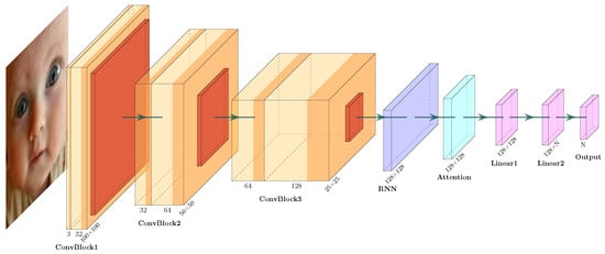
Figure 4.
Scheme of the developed convolutional neural network model with memory and attention.
Table 2.
General architecture of the proposed model and hyperparameters used in the experiments.
6. Data Augmentation
Before training, all input images are processed using a unified data augmentation pipeline designed to improve the model’s robustness to geometric and photometric variations. The transformations applied are
- Random horizontal flip with a probability of ;
- Random rotation within ;
- Random resized cropping to a fixed resolution of with a scaling factor sampled from ;
- Color jitter with brightness and contrast variations up to ;
- Conversion to tensor and normalization with mean and standard deviation .
This augmentation strategy increases sample diversity and improves generalization by making the model more robust to variations in pose, illumination, scale, and local image statistics.
7. Training Methodology
We address class imbalance using weighted cross-entropy:
where N is the dataset size, is the number of samples in class i, and are predicted probabilities. Training is performed with Adam, early stopping, and systematic hyperparameter search. Early stopping with patience of 30 epochs prevents overfitting. The dynamics of metrics in the learning process during the implementation of the described scenario is shown in Figure 5.
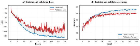
Figure 5.
Training dynamics: evolution of loss function and classification accuracy. (a) illustrates the progressive minimization of the cross-entropy loss function on both training (blue solid line) and validation (red line) datasets throughout the optimization process. The divergence between these curves after epoch N indicates the onset of model overfitting. (b) presents the corresponding classification accuracy metrics, demonstrating the model’s improving discriminative capability. The convergence gap between training and validation accuracy quantifies the generalization error of the proposed architecture.
The explored ranges include the learning rate , batch size , and dropout . The optimal configuration uses a learning rate of , batch size of 64, and dropout of . Since we needed to develop a strong and high-quality model to conduct a qualitative correction experiment, hyperparameters were selected based on maximizing classification accuracy in the validation sample. We attribute this relative stability to the model’s capacity and the rich, high-dimensional feature space it generates. This richness provides a robust foundation that is not easily destabilized by small parameter variations. The primary effect of hyperparameter tuning within this stable regime was on the dynamics and speed of convergence rather than on the final performance plateau.
8. Correction Mechanism
After training the base model, we extract multi-level representations (convolutional features, LSTM states, attention outputs, and pre-classification embeddings), forming dense descriptors for each sample. A gradient-boosted corrector (XGBoost, learning rate of , max depth of 5, subsample of , and 500 estimators) is trained on these descriptors to detect likely errors and adjust predictions when the confidence score falls below threshold . At this step, we also maximized the classification accuracy on the hyperparameter plane in order to obtain the strongest corrector. This mechanism acts as a meta-classifier, capturing feature interactions not fully modelled by the base network.
9. Results
This section presents the quantitative results of applying the proposed classification error correction method.
9.1. Metrics
Experimental Protocol: To evaluate our correction method, we employ a systematic class exclusion strategy. For each experiment, one emotion class is completely removed from training data, simulating real-world scenarios where new categories emerge after model deployment. We then measure the corrector’s ability to recover these excluded classes.
Key Evaluation: The primary metrics are Gain (Table 3) (ability to recover missing classes) and Retention (preservation of existing performance in Table 4).
Table 3.
Summary metrics of proofreader quality for each class. —the average change in the false positive error after applying the corrector. —the proportion of previously erroneous examples of the corrected class that were classified correctly.
Table 4.
Values of Harm and Retention metrics for all classes. The Harm metric reflects the proportion of examples that were correctly classified by the original model but became erroneous after applying the corrector. The Retention metric shows the proportion of correct predictions that remained after the correction. The values on the main diagonal are underlined and correspond to preserving/distorting predictions within the same class. The Retention and Harm metrics are also highlighted in red, which are higher and lower than the average, respectively.
The analysis was carried out using the metrics Retention, Harm, changes in Gain, and , as well as the integral performance characteristics listed below.
From the results shown in Table 4, it can be seen that the values of Retention remain high (close to unity) in all cases, which indicates that most of the correct predictions of the basic model are preserved. The values of Harm, on the contrary, record cases when the corrector introduces distortions. From Table 4, it can be seen that the corrector causes the most harm to the recognition of Fear(2) when correcting Surprise(1), Sadness(5) and Anger(6) when correcting Happiness(4), and Sadness(5) when correcting Neutral(7).
Summary indicators of the corrector’s effectiveness are given in Table 3. There is a positive trend for all classes Gain, which confirms the corrector’s ability to improve the completeness of the classification of the excluded class. The growth of remains relatively moderate, which makes the increase in Gain statistically significant. The greatest increases in quality are observed for ≪Happiness≫(4), ≪Surprise≫(1), ≪Disgust≫(3), and ≪Neutral≫(7), with greater increases observed for ≪Fear≫(2), ≪Sadness≫(5), and ≪Anger≫(6).
Table 5 shows the results of experiments to exclude classes from the training sample. In different cases, the correction allows for varying degrees of partial compensation for the loss of information about the excluded class.
Table 5.
Comparison of classification accuracy when using a corrector for different combinations of training classes. Values on the main diagonal represent accuracy for classes excluded from training—without correction, these would be 0, demonstrating the corrector’s ability to recover missing classes. The maximum values by row (the best prediction option for this class) are shown with underscores. The “Model 7 classes” column shows the accuracy of the original model without correction. Column P shows the value characterizing the effectiveness of the retraining correction relative to the case of complete retraining. The color coding reflects the quality of the compensation: green—high efficiency, orange—moderate, red—low.
For a formal assessment of the corrector’s contribution to the final quality of the classification, we introduce the corrector power indicator P, which is defined as the ratio of classification accuracy with correction to accuracy without correction:
Table 5 shows the values of the strength indicator of the corrector P. The best result was recorded for the class ≪Happiness≫ (), while for the classes ≪Sadness≫ and ≪Anger≫, the values of P are significantly lower (). This indicates a pronounced class dependence of the method’s effectiveness: for some emotions, correction successfully restores accuracy, while for others, the increase is lower. Thus, the error correction method is a promising tool. It is capable of increasing the stability of multiclass classifiers in conditions of incomplete and unbalanced samples, but its effectiveness depends on the class structure and requires further research.
9.2. Grad-CAM Analysis of LSTM Model
To gain insight into the regions of the face that drive the model’s predictions, we applied the Grad-CAM method to our trained LSTM-based network. The resulting activation maps highlight the facial areas most relevant for each emotion class.
As shown in Figure 6, the network focuses on the following regions:
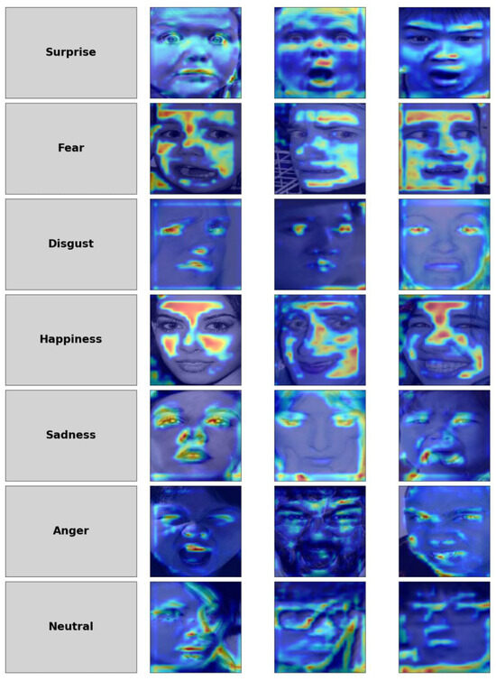
Figure 6.
Grad-CAM activation maps for each emotion class. Warmer colors indicate regions contributing most to the model’s predictions.
- Happiness: primarily cheeks and forehead.
- Joy: eyebrows and lips.
- Fear: eyebrows and cheeks.
- Disgust: eyes and mouth.
- Sadness: eyes and mouth.
- Anger: teeth and eyebrows.
- Neutral: distributed across the face; no single region is dominant.
These results are consistent with psychological studies of facial expressions and demonstrate that the model leverages key facial regions corresponding to human-recognizable emotion cues.
10. Computational Efficiency and Resource Requirements
A key advantage of the proposed post hoc correction method is its computational efficiency compared to full model retraining. Table 6 summarizes the main metrics for training time, inference time, and memory usage.
Table 6.
Computational efficiency and resource usage of the proposed method on NVIDIA RTX 4060 and 64 gb RAM.
As shown in Table 6, the corrector can be trained in a fraction of the time required for full model retraining while adding minimal inference overhead and negligible memory footprint. This ensures that the method scales efficiently with additional classes and remains suitable for real-time applications.
11. Discussion
Unlike traditional methods for handling class imbalance (e.g., focal loss and SMOTE) that operate during training, our method works in post hoc applications without modifying the base model. Unlike fine-tuning that requires full retraining, we avoid updating model parameters, making our approach suitable for deployed systems. While we demonstrated our method using CNN-LSTM, the correction approach is fundamentally model-agnostic. It relies on hidden representations that are available in any deep learning architecture (ResNet, Transformers, etc.), making it applicable across various domains beyond facial emotion recognition.
However, in the general case, correction turns out to be less effective than complete retraining and does not allow us to reach the level of a fully trained model. In turn, building a corrector is computationally much easier than completely retraining the model, and the proposed method allows one to create many correctors that implement a complex, nonlinear stack model. Further development of the approach may go in the following directions:
- Using more compact embeddings;
- Scaling experiments on large samples to increase stability;
- Developing adaptive correctors that take into account the semantic and statistical relationships of classes.
To better position our contribution within the state of the art, we contrast the proposed method with several alternative strategies. Full model retraining on data that includes the new class represents the most straightforward approach but requires access to the complete original dataset and substantial computational resources, and it risks catastrophic forgetting of previously learned classes. Our method, requiring only the pre-trained model and a small correction dataset, is orders of magnitude more efficient (Table 6) and preserves original class performance by design, as evidenced by high retention metrics.
Fine-tuning only the last layers of a pre-trained model offers greater efficiency than full retraining but still modifies the base model’s parameters through backpropagation and can degrade performance on original tasks. In contrast, our corrector operates as an additive, non-invasive module that leaves the base model unchanged. Post hoc class imbalance techniques such as loss re-weighting (e.g., focal loss) or sampling methods (e.g., SMOTE) are applied during training to improve minority class recognition but remain ineffective when a class is completely absent during training. Our approach specifically addresses this missing class scenario by leveraging the geometric properties of high-dimensional embeddings, as formalized by stochastic separation theorems.
The proposed post hoc error correction method aligns with stochastic separation theorems and multi-correctors from high-dimensional “postclassical” data analysis [21,22,24], enabling error handling on excluded classes via hidden representations without retraining, as demonstrated on RAF-DB with 0.811 gains on unseen emotion and 99% retention on a known emotion in the best setup. Unlike retraining, which demands full data access and epochs-long optimization risking resets on legacy performance, this leverages quasiorthogonality and “blessing of dimensionality” for low-computed, reversible corrections on granular cluster distributions. Fine-tuning offers partial adaptation but introduces forgetting and requires new labels, while class-imbalance techniques like resampling aid minorities yet falter on fully absent categories without separation theorems.
The proposed corrector introduces a trade-off: while it recovers missing classes (quantified by Gain), it can also misclassify previously correct predictions, as captured by the Harm metric (Table 4). A detailed analysis of these errors provides valuable insight into the method’s limitations and the semantic challenges of emotion recognition. The most pronounced Harm occurs in specific, interpretable patterns:
Fear (2) is most often harmed when correcting for Surprise (1). This aligns with psychological and visual similarity: both “Fear” and “Surprise” share wide eyes and raised eyebrows. The corrector, trained to identify patterns of the excluded “Surprise” class, may over-assign this label to ambiguous instances of “Fear” that lie close to the decision boundary in the embedding space. Anger (6) is frequently harmed when correcting for Happiness (Label 4). While these emotions are conceptually opposite, their intense expressions can share similar facial muscle tension and furrowing. The corrector for the highly distinctive “Happiness” class might misinterpret such high-activation “Anger” embeddings as out-of-distribution patterns for the trained set.
These failure modes reveal that the corrector’s effectiveness is constrained by the discriminative quality of the base model’s embeddings. We see the largest problem with emotion pairs that are visually or semantically confusable (e.g., fear/surprise). Future work could focus on making the corrector more conservative for such ambiguous cases or incorporating confidence thresholds to minimize harmful over-corrections.
12. Limitations and Future Work
Limitations:
- Performance depends on the discriminative power of the base model’s hidden representations;
- Storage of intermediate features is required during inference;
- Effectiveness varies with the visual distinctiveness of excluded classes.
Future Work:
- Extension to incremental learning with multiple new classes;
- Investigation of feature compression techniques for efficiency;
- Application to other domains such as medical imaging or security systems.
13. Conclusions
The results show that the proposed error correction method can significantly improve the quality of recognition of excluded classes while maintaining high accuracy on already known data. However, a significant dependence of efficiency on the nature of a particular class has been revealed.
High values of Retention indicate that the basic structure of the model’s predictions is preserved, and the risk of quality deterioration for the initial classes remains low. At the same time, the values Harm and demonstrate that the corrector can introduce undesirable distortions, especially in the case of emotions that are similar in feature space. Thus, the method has a positive effect but requires careful adjustment.
Experiments on class exclusion show that the corrector works especially successfully for classes with pronounced interclass similarity (for example, ≪Happiness≫), whereas for classes less related to others (for example, ≪Sadness≫ and ≪Anger≫), the effectiveness is noticeably lower.
Author Contributions
Conceptualization, S.V.S.; methodology, S.V.S. and A.A.L.; software, S.V.S. and A.A.L.; validation, S.V.S. and A.A.L.; formal analysis, A.A.L.; investigation, S.V.S. and A.A.L.; resources, S.V.S. and A.A.L.; data curation, S.V.S. and A.A.L.; writing—original draft preparation, S.V.S., A.A.L., and V.B.K.; writing—review and editing, S.V.S., A.A.L., and V.B.K.; visualization, A.A.L.; supervision, S.V.S.; project administration, S.V.S. and V.B.K.; funding acquisition, S.V.S. and V.B.K. All authors have read and agreed to the published version of the manuscript.
Funding
This work was carried out with the support of the federal assignment of the Ministry of Science and Higher Education of the Russian Federation (project No. FSMG-2025-0070).
Institutional Review Board Statement
Not applicable.
Informed Consent Statement
Not applicable.
Data Availability Statement
The dataset utilized in this study was downloaded from the Kaggle website and is available upon request at https://www.kaggle.com/datasets/shuvoalok/raf-db-dataset, accessed on 10 September 2025.
Conflicts of Interest
The authors declare no conflicts of interest.
References
- Tao, J.; Tan, T. Affective computing: A review. Int. J. Autom. Comput. 2005, 2, 302–312. [Google Scholar]
- Calvo, R.; D’Mello, S. Affect detection: An interdisciplinary review of models, methods, and their applications. IEEE Trans. Affect. Comput. 2010, 1, 18–37. [Google Scholar] [CrossRef]
- Liu, Y.; Fu, G. Emotion recognition by deeply learned multi-channel textual and EEG features. Future Gener. Comput. Syst. 2021, 119, 1–6. [Google Scholar] [CrossRef]
- Koelstra, S.; Muhl, C.; Soleymani, M.; Lee, J.; Yazdani, A.; Ebrahimi, T.; Pun, T.; Nijholt, A.; Patras, I. DEAP: A database for emotion analysis using physiological signals. IEEE Trans. Affect. Comput. 2012, 3, 18–31. [Google Scholar] [CrossRef]
- Sariyanidi, E.; Gunes, H.; Cavallaro, A. Automatic analysis of facial affect: A survey of registration, representation, and recognition. IEEE Trans. Pattern Anal. Mach. Intell. 2015, 37, 1113–1133. [Google Scholar] [CrossRef] [PubMed]
- Goodfellow, I.; Erhan, D.; Carrier, P.; Courville, A.; Mirza, M.; Hamner, B.; Cukierski, W.; Tang, Y.; Thaler, D.; Lee, D.; et al. Challenges in representation learning: A report on three machine learning contests. In Neural Information Processing; Springer: Berlin/Heidelberg, Germany, 2013; pp. 117–124. [Google Scholar]
- He, H.; Garcia, E. Learning from imbalanced data. IEEE Trans. Knowl. Data Eng. 2009, 21, 1263–1284. [Google Scholar] [CrossRef]
- Chawla, N.; Bowyer, K.; Hall, L.; Kegelmeyer, W. SMOTE: Synthetic minority over-sampling technique. J. Artif. Intell. Res. 2002, 16, 321–357. [Google Scholar] [CrossRef]
- Cui, Y.; Jia, M.; Lin, T.; Song, Y.; Belongie, S. Class-balanced loss based on effective number of samples. In Proceedings of the IEEE/CVF Conference on Computer Vision and Pattern Recognition, Long Beach, CA, USA, 15–20 June 2019; pp. 9268–9277. [Google Scholar]
- Lin, T.; Goyal, P.; Girshick, R.; He, K.; Dollár, P. Focal loss for dense object detection. In Proceedings of the IEEE International Conference on Computer Vision, Venice, Italy, 22–29 October 2017; pp. 2980–2988. [Google Scholar]
- Khan, S.; Hayat, M.; Zamir, S.; Shen, J.; Shao, L. Striking the right balance with uncertainty. IEEE Trans. Pattern Anal. Mach. Intell. 2019, 41, 2995–3007. [Google Scholar]
- Huang, C.; Li, Y.; Loy, C.C.; Tang, X. Deep imbalanced learning for face recognition and attribute prediction. IEEE Trans. Pattern Anal. Mach. Intell. 2019, 42, 2781–2794. [Google Scholar] [CrossRef]
- Hans, A.; Rao, S. A CNN-LSTM based deep neural networks for facial emotion detection in videos. Int. J. Adv. Signal Image Sci. 2021, 7, 11–20. [Google Scholar] [CrossRef]
- Rajpoot, A.S.; Panicker, M.R. Subject independent emotion recognition using EEG signals employing attention driven neural networks. Biomed. Signal Process. Control 2022, 75, 103547. [Google Scholar]
- Wang, K.; Peng, X.; Yang, J.; Meng, D.; Qiao, Y. Region attention networks for pose and occlusion robust facial expression recognition. IEEE Trans. Image Process. 2020, 29, 4057–4069. [Google Scholar] [CrossRef]
- Wang, L.; Zhang, L.; Qi, X.; Yi, Z. Deep attention-based imbalanced image classification. IEEE Trans. Neural Netw. Learn. Syst. 2021, 33, 3320–3330. [Google Scholar] [CrossRef]
- Altalhan, M.; Algarni, A.; Alouane, M. Imbalanced data problem in machine learning: A review. IEEE Access 2025, 13, 13686–13699. [Google Scholar] [CrossRef]
- Saurav, S.; Saini, R.; Singh, S. An integrated attention-guided deep convolutional neural network for facial expression recognition in the wild. Multimed. Tools Appl. 2025, 84, 10027–10069. [Google Scholar] [CrossRef]
- Huang, Q.; Huang, C.; Wang, X.; Jiang, F. Facial expression recognition with grid-wise attention and visual transformer. Inf. Sci. 2021, 580, 35–54. [Google Scholar] [CrossRef]
- Daihong, J.; Lei, D.; Jin, P. Facial expression recognition based on attention mechanism. Sci. Program. 2021, 2021, 6624251. [Google Scholar] [CrossRef]
- Gorban, A.; Grechuk, B.; Tyukin, I. Stochastic separation theorems: How geometry may help to correct AI errors. Not. Am. Math. Soc. 2023, 25–33. [Google Scholar] [CrossRef]
- Gorban, A.; Golubkov, A.; Grechuk, B.; Mirkes, E.; Tyukin, I. Correction of AI systems by linear discriminants: Probabilistic foundations. Inf. Sci. 2018, 466, 303–322. [Google Scholar] [CrossRef]
- Kovalchuk, A.; Lebedev, A.; Shemagina, O.; Nuidel, I.; Yakhno, V.; Stasenko, S. Enhancing Cascade Object Detection Accuracy Using Correctors Based on High-Dimensional Feature Separation. Technologies 2025, 13, 593. [Google Scholar] [CrossRef]
- Gorban, A.; Grechuk, B.; Mirkes, E.; Stasenko, S.; Tyukin, I. High-dimensional separability for one-and few-shot learning. Entropy 2021, 23, 1090. [Google Scholar] [CrossRef] [PubMed]
- Grechuk, B.; Gorban, A.; Tyukin, I. General stochastic separation theorems with optimal bounds. Neural Networks 2021, 138, 33–56. [Google Scholar] [CrossRef]
- Yi, W.; Sun, Y.; He, S. Data augmentation using conditional GANs for facial emotion recognition. In Proceedings of the 2018 Progress in Electromagnetics Research Symposium (PIERS-Toyama), Toyama, Japan, 1–4 August 2018; pp. 710–714. [Google Scholar]
- Chen, H.; Guo, C.; Li, Y.; Zhang, P.; Jiang, D. Semi-supervised multimodal emotion recognition with class-balanced pseudo-labeling. In Proceedings of the 31st ACM International Conference on Multimedia, Ottawa, ON, Canada, 29 October–3 November 2023; pp. 9556–9560. [Google Scholar]
- Shorten, C.; Khoshgoftaar, T.M. A survey on image data augmentation for deep learning. J. Big Data 2019, 6, 60. [Google Scholar] [CrossRef]
- Goodfellow, I.; Pouget-Abadie, J.; Mirza, M.; Xu, B.; Warde-Farley, D.; Ozair, S.; Courville, A.; Bengio, Y. Generative adversarial nets. In Advances in Neural Information Processing Systems; Curran Associates, Inc.: Red Hook, NY, USA, 2014; Volume 27. [Google Scholar]
- Koch, G.; Zemel, R.; Salakhutdinov, R. Siamese neural networks for one-shot image recognition. In Proceedings of the ICML Deep Learning Workshop, Lille, France, 6–11 July 2015; Volume 2. [Google Scholar]
- Chen, T.; Kornblith, S.; Norouzi, M.; Hinton, G. A simple framework for contrastive learning of visual representations. In Proceedings of the International Conference on Machine Learning, Virtual, 13–18 July 2020; pp. 1597–1607. [Google Scholar]
- Bengio, Y.; Louradour, J.; Collobert, R.; Weston, J. Curriculum learning. In Proceedings of the 26th Annual International Conference on Machine Learning, Montreal, QC, Canada, 14–18 June 2009; pp. 41–48. [Google Scholar]
- Chen, T.; Kornblith, S.; Swersky, K.; Norouzi, M.; Hinton, G.E. Big self-supervised models are strong semi-supervised learners. Adv. Neural Inf. Process. Syst. 2020, 33, 22243–22255. [Google Scholar]
- Li, S.; Deng, W.; Du, J. Reliable crowdsourcing and deep locality-preserving learning for expression recognition in the wild. In Proceedings of the IEEE Conference on Computer Vision and Pattern Recognition, Honolulu, HI, USA, 21–26 July 2017; pp. 2852–2861. [Google Scholar]
- Li, S.; Deng, W. RAF-DB DATASET. 2025. Available online: https://www.kaggle.com/datasets/shuvoalok/raf-db-dataset (accessed on 10 September 2025).
- Ming, Y.; Wang, J.; Zhang, J.; Li, H.; Liu, Y. CNN-LSTM facial expression recognition method fused with two-layer attention mechanism. Comput. Intell. Neurosci. 2022, 2022, 7450637. [Google Scholar] [CrossRef] [PubMed]


Disclaimer/Publisher’s Note: The statements, opinions and data contained in all publications are solely those of the individual author(s) and contributor(s) and not of MDPI and/or the editor(s). MDPI and/or the editor(s) disclaim responsibility for any injury to people or property resulting from any ideas, methods, instructions or products referred to in the content. |
© 2025 by the authors. Licensee MDPI, Basel, Switzerland. This article is an open access article distributed under the terms and conditions of the Creative Commons Attribution (CC BY) license.