Graph Attention Network with Mutual k-Nearest Neighbor Strategy for Predictive Maintenance in Nuclear Power Plants

Abstract

This study presents a graph-based framework for improving predictive maintenance in nuclear power plants (NPPs), integrating data balancing techniques with a proposed Graph Attention Network (GAT) with a Mutual k-Nearest Neighbor (Mk-NN) strategy, named GAT-Mk-NN. To enhance the system’s ability to discriminate between genuine faults and sensor anomalies, we introduce a novel procedure for generating synthetic false positives that simulate realistic sensor failures. To mitigate class imbalance, we employ structured oversampling and multiple synthetic data generation strategies. Our results demonstrate that our GAT-Mk-NN model achieves the best trade-off between accuracy and computational efficiency, reaching an F1-score of 0.882 and an accuracy of 0.884. Performance analysis reveals that low to moderate graph connectivity enhances both robustness and model generalization. Our GAT-Mk-NN model structure outperformed other state-of-the-art graph architectures (enhanced GCN, GraphSAGE, GIN, graph transformer, ChebNet, TAG, ARMA graph, simple GCN, GATv2, and hybrid GNN). The findings highlight the potential of graph-based learning for fault detection in sensor-dense industrial environments, offering actionable insights for deploying fault-tolerant diagnostics in critical systems.

1. Introduction

Fault identification in nuclear power plants (NPPs) is a critical component in ensuring operational safety, system reliability, and regulatory compliance [1]. Given the complexity and high-risk nature of nuclear facilities, early detection of faults can prevent catastrophic failures, reduce downtime, and optimize maintenance procedures [2]. Modern NPPs are equipped with a wide array of sensors that monitor variables such as temperature, pressure, radiation levels, vibration, and coolant flow in real-time. These sensors generate massive volumes of data, which, when properly analyzed, can reveal subtle patterns indicative of system degradation or imminent failure [3].

The integration of sensor networks into fault identification frameworks enables continuous monitoring and real-time diagnostics across various plant subsystems. By leveraging sensor data, it becomes possible to detect anomalies at early stages, differentiate between transient disturbances and critical faults, and localize the source of the issue with high accuracy [4]. Advanced signal processing, data fusion, graph-structured data, machine learning, and deep learning techniques are increasingly being employed to analyze this data, enabling the development of intelligent fault detection systems [5]. These systems enhance the decision-making process for operators and support predictive maintenance strategies, contributing to the overall safety and efficiency of nuclear energy generation [6].

The reliability of fault identification systems heavily depends on the accuracy and integrity of the sensor data [7]. A faulty sensor, whether due to calibration errors, hardware degradation, environmental interference, or communication failure, can lead to false alarms, missed fault detections, or incorrect system diagnoses [8]. In an NPP, such errors can have serious consequences, including unnecessary shutdowns, misinformed maintenance actions, or, in the worst cases, undetected critical faults that compromise plant safety. Therefore, distinguishing between actual system anomalies and sensor-related issues is essential, highlighting the need for robust sensor validation, redundancy, and fault-tolerant diagnostic algorithms [9].

To address the challenges posed by sensor faults and to enhance the robustness of fault identification in NPPs, this paper proposes a graph-based modeling framework. In this approach, the nuclear plant’s sensing infrastructure is represented as a graph, where each node corresponds to a sensor or monitored component, and edges encode physical or logical dependencies between them, such as shared subsystems, spatial proximity, or functional relationships. The graph-based structure enables the modeling of complex interconnections and mutual influences across the system, which are often overlooked in traditional linear diagnostic methods [10].

By utilizing this graph representation, it becomes feasible to detect inconsistencies between sensor readings and their expected values derived from the local neighborhood in the graph [11]. For example, suppose a temperature sensor reports an anomalous value that is not supported by adjacent pressure or flow sensors within the same subsystem. In such a case, it can be flagged as potentially faulty. These models can generalize fault patterns across different sections of the plant, distinguish between sensor malfunctions and actual process anomalies, and predict fault propagation paths through the network. This paradigm improves fault localization and classification and also enhances the reliability of condition monitoring in sensor-dense environments such as nuclear facilities [12].

Based on the potential of using graph models to classify faults, we propose an integrated framework to improve predictive maintenance in NPPs by leveraging synthetic data generation, class balancing, and Graph Neural Network (GNN) architectures. The proposed approach begins by simulating sensor faults through the generation of synthetic false positives, which mimic realistic sensor anomalies and help models learn to differentiate them from true system faults.

The methodology then applies advanced data balancing strategies to mitigate class imbalance, ensuring robust model training. The sensor network is represented as a graph, allowing the modeling of interdependencies between plant components. Our model considers a Graph Attention Network (GAT) with a Mutual k-Nearest Neighbor (k-NN) strategy, named GAT-Mk-NN. This model is compared to several GNN architectures across multiple graph construction techniques, aiming to ensure that the most effective strategy is used for fault detection. The main contributions of our proposed approach are as follows:

• Introducing a novel procedure to generate synthetic false positives, simulating sensor faults in NPP data. We propose structured oversampling techniques and multiple synthetic data generation strategies (boundary, interpolation, noise injection, feature corruption, hybrid) to handle class imbalance effectively.
• Modeling the sensor network of NPPs as graphs, capturing physical/logical dependencies between components for fault diagnosis. We perform an ablation study evaluating 11 GNN architectures and 11 graph construction methods, conducting 330 experiments using cross-validation on synthetic NPP data.
• Showing that low to moderate graph connectivity levels improve both performance and stability of the GNNs, and finding that the GAT combined with the mutual k-NN strategy achieves the best trade-off between accuracy and computational efficiency, with an F1-score of 0.882 and accuracy of 0.884.
• Presenting a rigorous statistical significance assessment, an explicit computational complexity analysis, and a detailed Pareto efficiency comparison. To support future evaluations, the dataset is available at https://github.com/SFStefenon/NPPmalfunctions (accessed on 21 December 2025), and the models evaluated in this paper are available at https://github.com/lseman/foreblocks (accessed on 21 December 2025).

This paper is organized as follows: in Section 2, related works are presented. Section 3 explains the procedure for creating false positives, which are indicative of a fault in the sensor and not in the system. In Section 4, the methodology of the proposed model is explained. The results of the application of the proposed method are presented and discussed in Section 5, and finally, in Section 6, the conclusions and directions for future work are presented.

2. Related Works

In recent years, the utilization of digital platforms for scenario simulation and safety assessment within the nuclear industry has gained increasing attention [13]. Prior studies have explored various modeling techniques to represent complex infrastructures such as NPPs, intending to enhance operational safety and efficiency [14]. A notable advancement in this domain is the introduction of a graph representation model tailored to simplify and structurally characterize NPPs for digital simulations [15]. This approach supports optimal planning within the plant environment, ultimately contributing to improved occupational safety. These advancements demonstrate the potential of graph-based methods as versatile tools for modeling, simulation, and decision-making in nuclear facilities [16].

Jyotish et al. [17] presented a Petri Net-based technique to evaluate system availability, addressing the limitations of traditional methods like Markov chains, reliability block diagrams, fault tree analyses, and flow networks. Their method involves modeling system behavior with Petri Net, generating a reachability graph, and deriving ordinary differential equations to quantify availability. Applied to the digital feed water control system of an NPP, including the failure and maintenance of main-steam safety valves, the technique achieved 99.20% accuracy, demonstrating its practical effectiveness.

Recognizing the limitations of existing deep learning approaches that mainly emphasize temporal features while neglecting spatial information, Wang et al. [18] propose a hierarchical deep learning model combining Fast Fourier Transform (FFT), Long Short-Term Memory networks (LSTM), and Graph Convolutional Networks (GCN). The FFT preprocesses sensor data to reduce volatility, LSTM extracts temporal features from historical sequences, and GCN automatically captures complex spatial relationships from multi-sensor inputs. Their model was validated through experiments using simulated data from the Personal Computer TRansient ANalyzer (PCTRAN), demonstrating superior diagnostic accuracy compared to individual models, thus offering an effective method to enhance fault detection and support operator decision-making in NPPs.

Zhang et al. [19] propose a novel approach named spatial–temporal graph conditionalized normalizing flows. The proposed model integrates multiscale dilated convolutional layers with mix-hopping graph convolutional layers to construct a spatio-temporal feature extractor. These features serve as conditional inputs for the normalizing flow model, while scheduling variables are incorporated to account for varying operating conditions. By analyzing anomaly variables through the conditional density magnitude, their method provides interpretable anomaly detection results. Validation on high-fidelity experimental bench data demonstrates that their model effectively detects and precisely localizes anomalies across different power modes, such as shutdown and peaking, outperforming existing approaches in handling complex operational scenarios.

Jyotish et al. [20] present a novel integrated methodology combining Petri Net modeling, reachability graph analysis, and ordinary differential equations to evaluate the reliability of safety-critical systems. The framework consists of sequential steps beginning with the Petri Net-based system modeling, from which both the ordinary differential equations and the reachability graph are generated. By identifying failure states within the reachability graph, the system’s reliability can be accurately assessed. The approach was applied to the shutdown system of an NPP and validated against the Brown and Lipow model, achieving an accuracy of 99.54%. Their method overcomes the state-space explosion problem common in traditional stochastic methods, which rely on predefined transition probabilities, thus offering a scalable and precise alternative for reliability evaluation in complex safety-critical infrastructures.

Liu et al. [21] propose a fault detection model based on GAT, designed to handle multiple simultaneous sensor faults. Their model first utilizes GAT to derive sensor correlation matrices, which are then input into an adversarial autoencoder for reconstruction. Simultaneously, the GAT node features are processed by an LSTM network to predict sensor ground truth values. Fault detection is achieved by computing an anomaly score that combines reconstruction and prediction errors. A fault decoupling strategy is introduced to identify multi-sensor faults by replacing faulty sensor data with model predictions, mitigating the negative effects of corrupted data on diagnosis. The model’s effectiveness was validated using simulated NPP data, with experimental results demonstrating improvements in accuracy and timeliness for multi-sensor fault detection and identification.

Chae et al. [22] propose a GNN-based accident diagnosis algorithm designed to deliver a high diagnostic resolution even with limited measurement data. The algorithm is trained using both physical correlation knowledge among plant components and available sensor measurements. To validate its effectiveness, multiple accident diagnosis tasks were conducted using limited measurement values, with performance compared against a Convolutional Neural Network (CNN). The results show that while both CNN and GNN performed well on low-resolution diagnosis tasks, the GNN significantly outperformed the CNN in scenarios demanding high diagnostic resolution, demonstrating its superior capability under data constraints.

Fei et al. [23] propose a novel video-level anomaly detection framework incorporating a latency mechanism that reduces false positives by flagging an anomaly only if it is detected consistently in the same region across consecutive video frames. This two-stage process begins with CNN-based scanning of sampled frames for anomaly types, followed by latency-based refinement of detection results. The framework’s effectiveness is demonstrated in a case study involving crack detection in superheater inspection videos, showing a significant reduction in false positives. Knowledge graphs are constructed to provide reasoning traceability, enhancing interpretability by illustrating why specific video segments are flagged as anomalous.

Existing inference algorithms struggle with efficiency when applied to large-scale systems exhibiting multiconnected and time-varying causalities. To address this, Dong and Zhou [24] propose methods for causality graph decomposition, simplification, and graphical transformation to reduce model complexity and generate a minimal causality graph. An event-oriented, early logical absorption algorithm is developed to optimize the logical reasoning process by minimizing computational costs during early-stage absorption operations. The algorithm’s effectiveness is validated using fault data from an NPP simulator, specifically focusing on the secondary loop model. The experimental results demonstrate that the proposed approach enhances the computational efficiency and fault diagnosis capability in large-scale dynamic systems.

Aminov et al. [25] introduce the integration of latent heat thermal energy storage systems into the thermal cycle of NPPs to facilitate load shifting. Graphs were developed to illustrate the relationship between the thermal power output of the latent heat thermal energy storage section and the duration of its discharge. These graphs, based on finite element modeling of unsteady heat transfer between lithium nitrate and water in finned and unfinned pipes, provide insights into the dynamic thermal performance of the storage system. They serve as a key tool for evaluating how long the system can supply useful thermal energy at varying power levels, supporting the design and optimization of the system under different operational conditions.

To enhance the reliability and sensitivity of online process monitoring in NPPs, Guohua et al. [26] propose an integrated approach combining thresholding, qualitative trend analysis, and signed directed graph inference. Initially, a threshold is employed for alarm generation, followed by signed directed graph backward inference to identify candidate faults from alarm parameters. The proposed methodology is validated through simulation experiments involving representative NPP accident scenarios such as loss of coolant accident, steam generator tube rupture, loss of feed water, main steam line break, and station blackout. The results demonstrate that the proposed method outperforms conventional approaches by enabling faster and more accurate fault diagnosis (

Table 1. Summary of related works in fault diagnosis and modeling for NPPs.

Work	Methodology	Model Type	Key Contribution/Application
[13]	Knowledge graph approach	Hybrid ontology extraction model	Integrates procedural and empirical knowledge, revealing hidden fault causality
[14]	Graph modeling of NPPs	Graph-based simulation	Structural representation for digital simulation and safety assessment
[15]	Graph representation for digital twins	Planning/graph model	Simplifies NPP modeling for operational planning
[16]	Interpretable GNN models	GNN + visualization	Enhances simulation explainability in NPPs
[17]	Petri Net + ODEs + reachability	Availability modeling	Achieves 99.20% accuracy; surpasses traditional reliability methods
[18]	FFT + LSTM + GCN hybrid	Spatio-temporal deep model	Improves NPP fault diagnosis using hybrid temporal-spatial features
[19]	Conditional normalizing flows + GCN	Probabilistic GNN	Localizes anomalies across varying NPP modes (shutdown, peaking)
[20]	Petri Net + reachability + ODEs	Reliability assessment	Validated NPP shutdown reliability with 99.54% accuracy
[21]	GAT + autoencoder + LSTM	Multi-sensor GNN model	Fault decoupling with robustness to simultaneous sensor faults
[22]	GNN accident diagnosis	GNN vs. CNN	Outperforms CNN in high-resolution diagnosis tasks with limited data
[23]	CNN + latency mechanism + KG	Vision-based anomaly detection	Reduces false positives in inspection videos with traceable reasoning
[24]	Causality graph decomposition + absorption	Logical inference model	Enhances fault inference speed and efficiency in dynamic systems
[25]	FEM thermal graphs for energy storage	Energy optimization model	Evaluates discharge duration and load-shifting capacity in NPPs
[26]	Thresholding + trend analysis + SDG	Hybrid rule-based diagnosis	Faster and more accurate NPP accident detection in simulations

).

3. False Positive Generation and Dataset Balancing Strategy

This section explains the strategy for creating false positives, which are represented by faulty sensors. A faulty sensor is defined here as a sensor that shows a measurement that is not consistent with what is happening in the generation process at the thermonuclear power plant. To simulate this condition, experiments are carried out with the PCTRAN simulator [27]. To improve the classification capacity of the models, a balancing strategy is applied, as explained in detail in this section.

Let $\mathcal{D}={\left\{({\mathbf{x}}_i,y_i)\right\}}_{i=1}^N$ represent our original dataset, where ${\mathbf{x}}_i\in {\mathbb{R}}^d$ are d-dimensional feature vectors and $y_i\in \{0,1\}$ are binary labels representing normal operation ($y_i=0$) and fault conditions ($y_i=1$), respectively. The dataset partitions into three components: normal operation samples ${\mathcal{D}}_{\mathrm{normal}}={\left\{({\mathbf{x}}_i,0)\right\}}_{i=1}^{N_0}$, fault condition samples ${\mathcal{D}}_{\mathrm{fault}}={\left\{({\mathbf{x}}_i,1)\right\}}_{i=1}^{N_1}$, and synthetically generated false positive samples ${\mathcal{D}}_{\mathrm{fp}}={\left\{({\mathbf{x}}_i,0)\right\}}_{i=1}^{N_{\mathrm{fp}}}$.

Before generating false positives, we perform a statistical analysis of the existing data distributions to inform our generation strategy. For each feature dimension $j\in \{1,2,\dots ,d\}$, we compute the statistical moments for both classes:

$$\begin{array}{c}\hfill {\mu }_{0,j}={\displaystyle \frac{1}{N_0}}\sum _{i=1}^{N_0}{\mathbf{x}}_{i,j}^{\left(0\right)},{\sigma }_{0,j}^2={\displaystyle \frac{1}{N_0-1}}\sum _{i=1}^{N_0}{({\mathbf{x}}_{i,j}^{\left(0\right)}-{\mu }_{0,j})}^2\end{array}$$

(1)

$$\begin{array}{c}\hfill {\mu }_{1,j}={\displaystyle \frac{1}{N_1}}\sum _{i=1}^{N_1}{\mathbf{x}}_{i,j}^{\left(1\right)},{\sigma }_{1,j}^2={\displaystyle \frac{1}{N_1-1}}\sum _{i=1}^{N_1}{({\mathbf{x}}_{i,j}^{\left(1\right)}-{\mu }_{1,j})}^2\end{array}$$

(2)

where ${\mathbf{x}}_{i,j}^{\left(0\right)}$ and ${\mathbf{x}}_{i,j}^{\left(1\right)}$ denote the j-th feature of the i-th sample from normal and fault classes, respectively.

To quantify the separability between classes for each feature, we compute Cohen’s d effect size:

$$\begin{array}{c}\hfill d_j={\displaystyle \frac{|{\mu }_{1,j}-{\mu }_{0,j}|}{\sqrt{\frac{{\sigma }_{0,j}^2+{\sigma }_{1,j}^2}{2}}}}.\end{array}$$

(3)

The separation difficulty for feature j is categorized as very hard ($d_j<0.2$), hard ($0.2\le d_j<0.5$), medium ($0.5\le d_j<0.8$), or easy ($d_j\ge 0.8$). We also define the overlap potential as ${\rho }_j={\displaystyle \frac{1}{1+d_j}}$, where higher values indicate greater potential for generating challenging false positives in feature dimension j.

3.1. False Positive Generation Strategies

We implement five distinct strategies for generating synthetic false positive samples that are labeled as normal but exhibit characteristics that may challenge classification algorithms. Each strategy targets different aspects of the decision boundary and data distribution characteristics.

• Boundary Method: Generates samples near the decision boundary by moving normal samples toward the fault region: ${\mathbf{x}}_{\mathrm{fp}}^{\left(b\right)}={\mathbf{x}}_{\mathrm{normal}}+\alpha ·({\mu }_1-{\mathbf{x}}_{\mathrm{normal}})$, where ${\mathbf{x}}_{\mathrm{normal}}$ is a randomly selected normal sample, ${\mu }_1={[{\mu }_{1,1},{\mu }_{1,2},\dots ,{\mu }_{1,d}]}^T$ is the fault class centroid, and $\alpha \sim \mathcal{U}(0.2,0.4)$ controls the movement magnitude. Movement is applied selectively to features with medium separation difficulty: ${\mathcal{F}}_{\mathrm{medium}}=\{j:{\mathrm{difficulty}}_j\in \{\mathrm{medium},\mathrm{hard}\}\}$.
• Interpolation Method: Creates ambiguous regions through linear interpolation between normal and fault samples: ${\mathbf{x}}_{\mathrm{fp}}^{\left(i\right)}=(1-\beta ){\mathbf{x}}_{\mathrm{normal}}+\beta {\mathbf{x}}_{\mathrm{fault}}+ϵ$, where $\beta \sim \mathrm{Beta}(2,5)$ (biased toward normal), and $ϵ\sim \mathcal{N}(\mathbf{0},{0.05}^2{\Sigma }_0)$ is Gaussian noise with covariance ${\Sigma }_0$ derived from normal samples.
• Noise Injection Method: Applies structured noise patterns that may be mistaken for anomalies: ${\mathbf{x}}_{\mathrm{fp}}^{\left(n\right)}={\mathbf{x}}_{\mathrm{normal}}+\eta$. The noise vector $\eta$ uses three patterns: spike noise ${\eta }_j\sim \mathcal{N}(0,{\left(3\gamma {\sigma }_{0,j}\right)}^2)$, drift noise ${\eta }_j\sim \mathcal{U}(-2\gamma {\sigma }_{0,j},2\gamma {\sigma }_{0,j})$, and oscillation noise ${\eta }_j=\gamma {\sigma }_{0,j}sin\left({\varphi }_j\right)$ where ${\varphi }_j\sim \mathcal{U}(0,2\pi )$.
• Feature Corruption Method: Performs selective replacement of normal features with fault-distributed values: ${\mathbf{x}}_{\mathrm{fp},j}^{\left(c\right)}=\left\{\begin{array}{cc}{\mathbf{x}}_{\mathrm{normal},j}\hfill & \mathrm{if}j\notin \mathcal{C}\hfill \\ {\mathbf{x}}_{\mathrm{fault},k}\hfill & \mathrm{if}j\in \mathcal{C}\hfill \end{array}\right.$, where $\mathcal{C}\subset \{1,2,\dots ,d\}$ is a randomly selected subset with $\left|\mathcal{C}\right|=max(1,\lfloor d/3\rfloor )$, biased toward easily separable features, $P(j\in \mathcal{C})\propto \mathbb{I}[{\mathrm{difficulty}}_j\in \{\mathrm{easy},\mathrm{medium}\}]$.
• Hybrid Method: Combines multiple strategies using weighted sampling: ${\mathbf{x}}_{\mathrm{fp}}^{\left(h\right)}\sim {\sum }_{m\in \mathcal{M}}{w}_m·{\mathrm{Method}}_m$, where $\mathcal{M}=\{\mathrm{boundary},\mathrm{interpolation},\mathrm{noise},\mathrm{corruption}\}$ and weights $\mathbf{w}=[0.3,0.3,0.2,0.2]$.

3.2. Adaptive Strategy Selection

The optimal false positive generation strategy is selected based on data characteristics and desired challenge level. Given the quality target $\tau$ and average effect size $\overline{d}={\displaystyle \frac{1}{d}}{\sum }_{j=1}^d{d}_j$, we select strategies according to

$$\mathrm{Strategy}=\left\{\begin{array}{cc}\mathrm{noise\_injection}\hfill & \mathrm{if}\tau =\mathrm{easy}\hfill \\ \mathrm{boundary}\hfill & \mathrm{if}\tau =\mathrm{realistic}\wedge \overline{d}>0.8\hfill \\ \mathrm{interpolation}\hfill & \mathrm{if}\tau =\mathrm{realistic}\wedge \overline{d}\le 0.8\hfill \\ \mathrm{feature\_corruption}\hfill & \mathrm{if}\tau =\mathrm{challenging}\wedge \exists j:d_j<0.5\hfill \\ \mathrm{hybrid}\hfill & \mathrm{otherwise}.\hfill \end{array}\right.$$

This adaptive approach ensures that the generated false positives match the intended difficulty level while respecting the underlying data distribution characteristics.

3.3. Dataset Balancing Strategy

Given class counts $N_0$ and $N_1$, we define the imbalance ratio $\lambda =max(N_0,N_1)/min(N_0,N_1)$ and select balancing methods based on dataset characteristics. The balancing strategy is as follows: no balancing for $\lambda <1.5$, oversampling for $1.5\le \lambda <3.0$, undersampling for $\lambda \ge 3.0$ when $N_{\mathrm{total}}>1000$, and oversampling otherwise. The sampling considers the following tasks:

• Multi-Strategy Oversampling: For the minority class, we generate $N_{\mathrm{add}}=N_{\max }-N_{\min }$ additional samples using three approaches with probabilities $P\left(\mathrm{resample}\right)=0.6$, considering $P\left(\mathrm{noise\_augmentation}\right)=0.2$, and $P\left(\mathrm{interpolation}\right)=0.2$. Noise augmentation follows ${\mathbf{x}}_{\mathrm{aug}}={\mathbf{x}}_{\mathrm{original}}+\xi$, where $\xi \sim \mathcal{N}(\mathbf{0},{0.1}^2{\Sigma }_{\mathrm{class}})$, while interpolation uses ${\mathbf{x}}_{\mathrm{aug}}=\alpha {\mathbf{x}}_i+(1-\alpha ){\mathbf{x}}_k$ with $\alpha \sim \mathcal{U}(0.2,0.8)$.
• Intelligent Undersampling: For the majority class, we apply k-means clustering with $k=N_{\min }$ to obtain clusters $\mathcal{C}=\{C_1,C_2,\dots ,C_k\}$, then select the sample closest to each centroid: ${\mathbf{x}}_{\mathrm{selected}}^{\left(i\right)}=arg{min}_{\mathbf{x}\in C_i}{\parallel \mathbf{x}-{\mu }_i\parallel }_2$. This preserves diversity while reducing class size.
• Synthetic Minority Oversampling Technique-like Synthesis: For small datasets, each minority sample ${\mathbf{x}}_i$ generates synthetic samples through ${\mathbf{x}}_{\mathrm{synthetic}}={\mathbf{x}}_i+\alpha ({\mathbf{x}}_{\mathrm{neighbor}}-{\mathbf{x}}_i)$, with ${\mathbf{x}}_{\mathrm{neighbor}}$ from the k nearest neighbors ${\mathcal{N}}_k\left({\mathbf{x}}_i\right)$ and $\alpha \sim \mathcal{U}(0,1)$.

3.4. Quality Validation and Assessment

For the generated false positives ${\mathcal{D}}_{\mathrm{fp}}$, we compute similarity metrics to assess quality. The similarity to normal and fault classes for feature j are defined as

$$\begin{array}{c}\hfill S_{\mathrm{normal}}^{\left(j\right)}={\displaystyle \frac{1}{1+\frac{1}{N_{\mathrm{fp}}}{\sum }_{i=1}^{N_{\mathrm{fp}}}|{\mathbf{x}}_{\mathrm{fp},i,j}-{\mu }_{0,j}|}}\end{array}$$

(4)

and

$$\begin{array}{c}\hfill S_{\mathrm{fault}}^{\left(j\right)}={\displaystyle \frac{1}{1+\frac{1}{N_{\mathrm{fp}}}{\sum }_{i=1}^{N_{\mathrm{fp}}}|{\mathbf{x}}_{\mathrm{fp},i,j}-{\mu }_{1,j}|}},\end{array}$$

(5)

respectively. The overall quality score combines these measures:

$$\begin{array}{c}\hfill Q=0.7·{\displaystyle \frac{1}{d}}\sum _{j=1}^d{S}_{\mathrm{normal}}^{\left(j\right)}+0.3·{\displaystyle \frac{1}{d}}\sum _{j=1}^d{S}_{\mathrm{fault}}^{\left(j\right)}.\end{array}$$

(6)

The generated samples are validated against multiple criteria: bounds checking ensures $min({\mathcal{D}}_{\mathrm{normal}}\cup {\mathcal{D}}_{\mathrm{fault}})\le {\mathbf{x}}_{\mathrm{fp}}\le max({\mathcal{D}}_{\mathrm{normal}}\cup {\mathcal{D}}_{\mathrm{fault}})$, finite value verification confirms ${\mathbf{x}}_{\mathrm{fp}}\in {\mathbb{R}}^d$ with no NaN or infinite values, and quality thresholding maintains $0.4\le Q\le 0.9$ to ensure challenging but not degenerate samples.

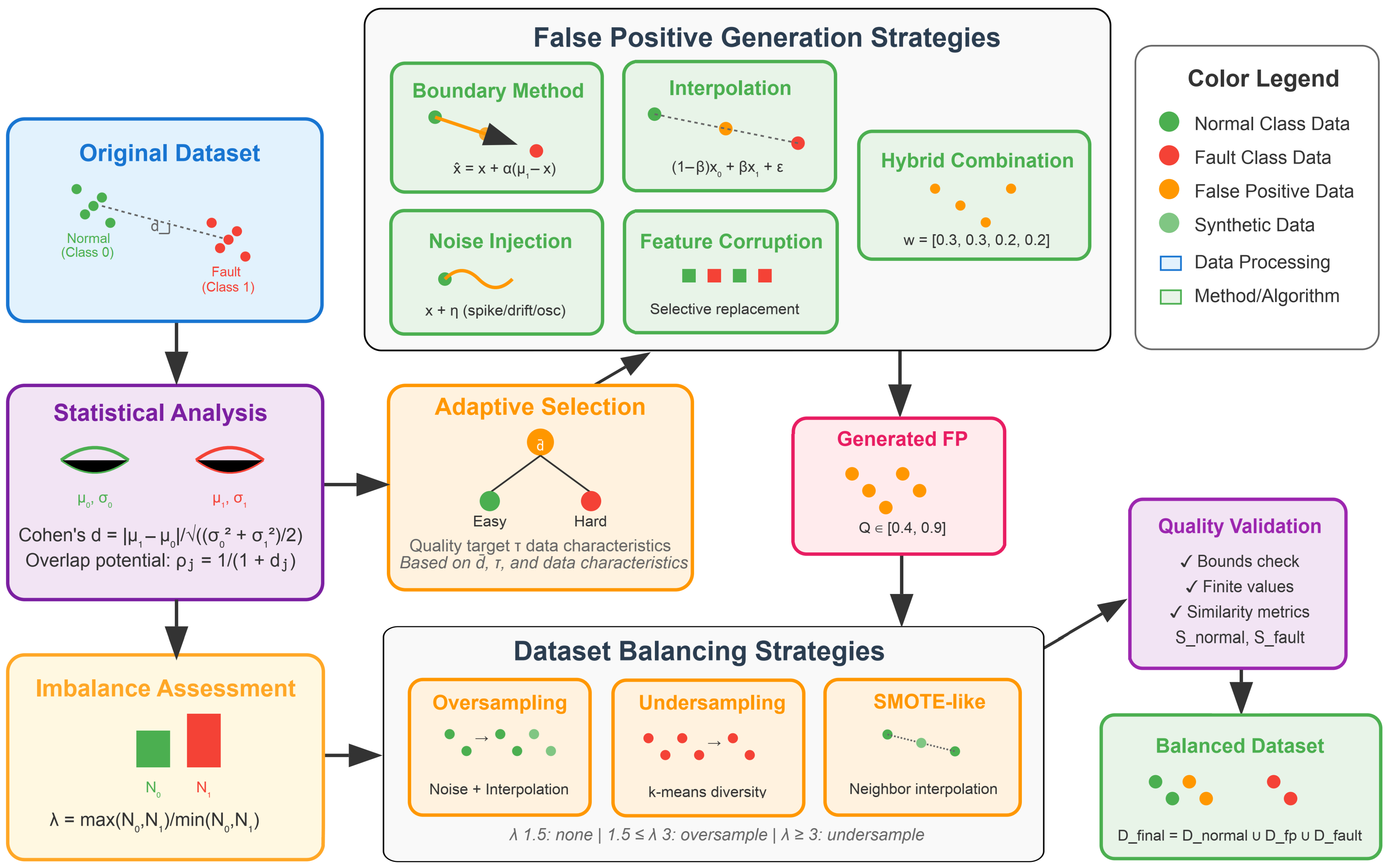
Figure 1 presents the summarized methodology for creating false positive samples. Initially, a statistical analysis is conducted to interpret the data, after which an optional sample selection is performed to create false positives. After selecting the data, a balancing strategy is carried out to ensure that the dataset does not have large unbalances between classes. Finally, the samples are validated, and the new dataset is determined.

4. Methodology

Graph Neural Networks (GNNs) operate by aggregating and transforming information from a node’s local neighborhood within a graph structure [28]. This inherently layered and modular nature of GNNs makes them ideal candidates for ablation analysis. By selectively disabling or modifying specific components (e.g., removing edge features, reducing message-passing steps, or eliminating non-linear transformations), it is possible to better understand which parts of the architecture drive performance improvements or introduce vulnerabilities such as overfitting or instability.

4.1. Graph Neural Network Fundamentals

GNNs operate on graph-structured data $\mathcal{G}=(\mathcal{V},\mathcal{E},\mathbf{X})$, where $\mathcal{V}=\{v_1,v_2,\dots ,v_N\}$ is the set of nodes, $\mathcal{E}\subseteq \mathcal{V}\times \mathcal{V}$ is the set of edges, and $\mathbf{X}\in {\mathbb{R}}^{N\times d}$ represents node features. GNNs use the iterative message passing framework, where node representations are updated by aggregating information from their local neighborhoods [29].

The general message passing paradigm follows a two-step process at each layer l, the message computation and the node update. For message computation, each edge $(i,j)\in \mathcal{E}$, a message is computed as

$$\begin{array}{c}\hfill {\mathbf{m}}_{i\leftarrow j}^{\left(l\right)}={\varphi }^{\left(l\right)}\left({\mathbf{h}}_i^{(l-1)},{\mathbf{h}}_j^{(l-1)},{\mathbf{e}}_{ij}\right)\end{array}$$

(7)

where ${\varphi }^{\left(l\right)}$ is a learnable message function, ${\mathbf{h}}_i^{(l-1)}$ represents the node features at layer $l-1$, and ${\mathbf{e}}_{ij}$ are optional edge features. Node representations are updated by aggregating messages from neighbors:

$$\begin{array}{c}\hfill {\mathbf{h}}_i^{\left(l\right)}={\psi }^{\left(l\right)}\left({\mathbf{h}}_i^{(l-1)},\mathrm{AGG}\left(\left\{{\mathbf{m}}_{i\leftarrow j}^{\left(l\right)}:j\in \mathcal{N}\left(i\right)\right\}\right)\right)\end{array}$$

(8)

where ${\psi }^{\left(l\right)}$ is an update function, $\mathcal{N}\left(i\right)=\{j:(i,j)\in \mathcal{E}\}$ denotes the neighborhood of node i, and AGG is a permutation-invariant aggregation function such as sum, mean, or max. The advantages of this framework include:

• Permutation Invariance: The output is invariant to node ordering due to the symmetric aggregation operation.
• Inductive Learning: Models can generalize to unseen graph structures during inference.
• Locality Preservation: Each layer captures information from immediate neighbors, with deeper networks accessing wider neighborhoods through multiple hops.
• Parameter Sharing: The same learned functions $\varphi$ and $\psi$ are applied across all nodes, enabling scalability to graphs of varying sizes.

For node classification tasks, the final node representations ${\mathbf{h}}_i^{\left(L\right)}$ after L layers are passed through a classifier to obtain predictions:

$$\begin{array}{c}\hfill {\widehat{\mathbf{y}}}_i=\mathrm{softmax}\left({\mathbf{W}}_{\mathrm{out}}{\mathbf{h}}_i^{\left(L\right)}+{\mathbf{b}}_{\mathrm{out}}\right)\end{array}$$

(9)

where ${\mathbf{W}}_{\mathrm{out}}\in {\mathbb{R}}^{C\times d_L}$ and ${\mathbf{b}}_{\mathrm{out}}\in {\mathbb{R}}^C$ are learnable parameters for C classes [30].

Given the preprocessed and balanced dataset ${\mathcal{D}}_{\mathrm{final}}={\left\{({\mathbf{x}}_i,y_i)\right\}}_{i=1}^N$ where ${\mathbf{x}}_i\in {\mathbb{R}}^d$ are feature vectors and $y_i\in \{0,1\}$ are binary labels, we construct a graph $\mathcal{G}=(\mathcal{V},\mathcal{E})$ where each data point corresponds to a node $v_i\in \mathcal{V}$ and edges $\mathcal{E}$ represent relationships between samples.

4.2. Mutual k-NN Graph

The k-Nearest Neighbor (k-NN) graph [31] construction method connects each node to its k nearest neighbors in the feature space based on Euclidean distance. This approach captures local similarities and is particularly effective for maintaining manifold structure in high-dimensional data. For each node $v_i$, we define the k-NN set as

$$\begin{array}{c}\hfill {\mathcal{N}}_k\left(i\right)=arg\underset{S\subset \{1,\dots ,N\},\left|S\right|=k}{min}\sum _{j\in S}{\parallel {\mathbf{x}}_i-{\mathbf{x}}_j\parallel }_2.\end{array}$$

(10)

The resulting edge set is

$$\begin{array}{c}\hfill {\mathcal{E}}_{\mathrm{knn}}=\{(i,j):j\in {\mathcal{N}}_k\left(i\right)\}.\end{array}$$

(11)

The k-NN graph ensures that each node has exactly k outgoing edges, resulting in a directed graph with uniform out-degree [32]. The time complexity is $O\left(N^{2}d\right)$ for an exhaustive search or $O(NlogN·d)$ using efficient nearest neighbor algorithms like KD-trees or LSH. This construction preserves local neighborhood structure and is based on the manifold hypothesis that high-dimensional data lies on or near a low-dimensional manifold. The parameter k controls the locality–globality trade-off: a small k preserves the fine-grained local structure but may create disconnected components, while a large k increases connectivity but may introduce noise [33].

The mutual k-NN graph enforces bidirectional nearest neighbor relationships, creating a symmetric graph where edges exist only if both nodes are in each other’s k-NN.

$$\begin{array}{c}\hfill {\mathcal{E}}_{\mathrm{mutual}}=\{(i,j):j\in {\mathcal{N}}_k\left(i\right)\wedge i\in {\mathcal{N}}_k\left(j\right)\}\end{array}$$

(12)

This construction typically results in a sparser graph than a standard k-NN with variable degrees. The mutual constraint ensures stronger local relationships and natural symmetry. The average degree is typically much less than k. The mutual k-NN reduces spurious connections by requiring bidirectional similarity, leading to a more robust graph structure. This is valuable when dealing with boundary points between clusters or regions with different densities [34].

In this work, the k-NN graph, epsilon-ball graph [35], cosine similarity graph [36], correlation-based graph [37], RBF graph [38], adaptive k-NN graph [39], Delaunay triangulation graph [40], Gabriel graph [41], Relative Neighborhood Graph (RNG) [42], and radius graph [43] are considered for comparison to the mutual k-NN graph.

4.3. Feature Processing and Node Representations

The input features undergo standardization to ensure numerical stability and fair comparison across different scales:

$$\begin{array}{c}\hfill {\tilde{\mathbf{x}}}_i={\displaystyle \frac{{\mathbf{x}}_i-\mu }{\sigma }}\end{array}$$

(13)

where $\mu ={\displaystyle \frac{1}{N}}{\sum }_{i=1}^N{\mathbf{x}}_i$ and ${\sigma }^2={\displaystyle \frac{1}{N-1}}{\sum }_{i=1}^N{({\mathbf{x}}_i-\mu )}^2$. The feature matrix $\mathbf{X}={[{\tilde{\mathbf{x}}}_1,{\tilde{\mathbf{x}}}_2,\dots ,{\tilde{\mathbf{x}}}_N]}^T\in {\mathbb{R}}^{N\times d}$ serves as node attributes in the graph neural networks.

Graph Attention Network (GAT)

GAT introduces attention mechanisms to graph neural networks, allowing nodes to attend to their neighbors with different weights based on the relevance of their features.   

$$\begin{array}{c}\hfill {\mathbf{h}}_i^{(l+1)}{=\parallel }_{k=1}^K\sigma \left(\sum _{j\in \mathcal{N}\left(i\right)\cup \left\{i\right\}}{\alpha }_{ij}^{\left(k\right)}{\mathbf{W}}^{\left(k\right)}{\mathbf{h}}_j^{\left(l\right)}\right)\end{array}$$

(14)

where the attention weights are computed as

$$\begin{array}{c}\hfill {\alpha }_{ij}^{\left(k\right)}={\displaystyle \frac{exp\left(\mathrm{LeakyReLU}\left({\mathbf{a}}^{\left(k\right)T}[{\mathbf{W}}^{\left(k\right)}{\mathbf{h}}_i^{\left(l\right)}\parallel {\mathbf{W}}^{\left(k\right)}{\mathbf{h}}_j^{\left(l\right)}]\right)\right)}{{\sum }_{m\in \mathcal{N}\left(i\right)\cup \left\{i\right\}}exp\left(\mathrm{LeakyReLU}\left({\mathbf{a}}^{\left(k\right)T}[{\mathbf{W}}^{\left(k\right)}{\mathbf{h}}_i^{\left(l\right)}\parallel {\mathbf{W}}^{\left(k\right)}{\mathbf{h}}_m^{\left(l\right)}]\right)\right)}}\end{array}$$

(15)

and ‖ denotes concatenation across K attention heads.

The attention mechanism provides a learnable, adaptive aggregation function that can focus on the most relevant neighbors. Multi-head attention allows the model to attend to different aspects of the neighbor representations simultaneously. GAT addresses the limitation of fixed aggregation functions in traditional GCNs by learning to weight neighbor contributions dynamically. This is particularly valuable in heterogeneous graphs or when different neighbors have varying relevance to the prediction task [44].

There are currently several state-of-the-art GNN models applied to graph-based data classification. In this paper, the enhanced GCN [45], GraphSAGE (Sample and Aggregate) [46], Graph Isomorphism Network (GIN) [47], Graph transformer [48], Chebyshev graph Network (ChebNet) [49], Topology Adaptive GCN (TAG) [50], AutoRegressive Moving Average (ARMA) graph [51], simple GCN [52], GATv2 [53], and hybrid GNN [54] models were compared.

4.4. Training Protocol and Optimization

We employ stratified k-fold cross-validation with $k=5$ to ensure balanced class distribution across folds. For each fold, the training procedure optimizes the cross-entropy loss function:

$$\begin{array}{c}\hfill \mathcal{L}=-{\displaystyle \frac{1}{|{\mathcal{V}}_{\mathrm{train}}|}}\sum _{i\in {\mathcal{V}}_{\mathrm{train}}}\sum _{c=1}^C{y}_{ic}log\left({\widehat{y}}_{ic}\right)\end{array}$$

(16)

where ${\widehat{y}}_{ic}=\mathrm{softmax}{\left({\mathbf{z}}_i\right)}_c$ and ${\mathbf{z}}_i$ is the final node representation.

The optimization process uses the Adam optimizer with adaptive learning rate:

$$\begin{array}{cc}\hfill {\mathbf{m}}_t& ={\beta }_1{\mathbf{m}}_{t-1}+(1-{\beta }_1){\nabla }_{\theta }\mathcal{L}\hfill \end{array}$$

(17)

$$\begin{array}{cc}\hfill {\mathbf{v}}_t& ={\beta }_2{\mathbf{v}}_{t-1}+(1-{\beta }_2){\left({\nabla }_{\theta }\mathcal{L}\right)}^2\hfill \end{array}$$

(18)

$$\begin{array}{cc}\hfill {\theta }_{t+1}& ={\theta }_t-{\displaystyle \frac{\alpha }{\sqrt{{\mathbf{v}}_t}+ϵ}}{\mathbf{m}}_t\hfill \end{array}$$

(19)

with learning rate $\alpha =0.01$, momentum parameters ${\beta }_1=0.9$ and ${\beta }_2=0.999$, and weight decay $\lambda =5\times {10}^{-4}$. The training features are as follows:

• Automatic Mixed Precision: Reduces memory usage and accelerates training using FP16 operations where numerically stable, with automatic loss scaling to prevent gradient underflow.
• Early Stopping: Training terminates when validation loss fails to improve for $p=10$ consecutive epochs with minimum improvement threshold $\delta ={10}^{-4}$:

  $$\begin{array}{c}\hfill \mathrm{Stop}\mathrm{if}{\mathcal{L}}_{\mathrm{val}}^{\left(t\right)}-{\mathcal{L}}_{\mathrm{val}}^{(t-p)}>-\delta \end{array}$$

  (20)
• Learning Rate Scheduling: ReduceLROnPlateau reduces the learning rate when the validation loss plateaus:

  $$\begin{array}{c}\hfill {\alpha }_{\mathrm{new}}={\alpha }_{\mathrm{old}}\times \mathrm{factor}\mathrm{if}\mathrm{no}\mathrm{improvement}\mathrm{for}\mathrm{patience}\mathrm{epochs}\end{array}$$

  (21)

  with patience = 5 and factor = 0.5.
• Gradient Scaling: Prevents gradient underflow in mixed-precision training through dynamic loss scaling.

4.5. Ablation Study Design and Statistical Analysis

The ablation experiment systematically evaluates $11\times 11=121$ model–graph combinations across 5-fold cross-validation, resulting in $121\times 5=605$ individual training runs. This comprehensive design ensures robust statistical conclusions about the relative performance of different approaches. In the performance aggregation, for each combination $(m,g)$ of model m and graph method g, we compute sample statistics:

$$\begin{array}{cc}\hfill {\overline{\mu }}_{m,g}& ={\displaystyle \frac{1}{K}}\sum _{k=1}^K{\mathrm{Metric}}_{m,g,k}\hfill \end{array}$$

(22)

$$\begin{array}{cc}\hfill {\sigma }_{m,g}^2& ={\displaystyle \frac{1}{K-1}}\sum _{k=1}^K{({\mathrm{Metric}}_{m,g,k}-{\overline{\mu }}_{m,g})}^2\hfill \end{array}$$

(23)

where $K=5$ is the number of cross-validation folds.

We employ paired t-tests to compare performance differences:

$$\begin{array}{c}\hfill t={\displaystyle \frac{\overline{d}}{\frac{s_d}{\sqrt{K}}}}\end{array}$$

(24)

where $\overline{d}$ is the mean difference between paired samples and $s_d$ is the sample standard deviation of differences. Models and graph methods are ranked by average F1-score, with confidence intervals of

$$\begin{array}{c}\hfill C{I}_{95\%}=\overline{\mu }\pm t_{K-1,0.025}·{\displaystyle \frac{\sigma }{\sqrt{K}}}\end{array}$$

(25)

where $t_{K-1,0.025}$ is the critical value from the t-distribution with $K-1$ degrees of freedom.

To analyze the size effect, Cohen’s d quantifies the magnitude of performance differences:

$$\begin{array}{c}\hfill d={\displaystyle \frac{{\overline{\mu }}_1-{\overline{\mu }}_2}{\sqrt{\frac{(K-1)s_1^2+(K-1)s_2^2}{2K-2}}}}.\end{array}$$

(26)

The computational complexity analysis is based on the training time evaluation, which considers the parameter count, given by

$$\begin{array}{c}\hfill \left|\theta \right|=\sum _{l=1}^L{d}_l\times d_{l+1}+\sum _{l=1}^L{d}_{l+1}\end{array}$$

(27)

where the first term accounts for weight matrices and the second for bias vectors.

The graph connectivity is evaluated by the average node degree and its impact on computational cost, calculated by

$$\begin{array}{c}\hfill \overline{d}={\displaystyle \frac{2\left|\mathcal{E}\right|}{N}}.\end{array}$$

(28)

The time complexity per layer is

$$\begin{array}{c}\hfill {\mathcal{O}}_{\mathrm{layer}}=\mathcal{O}\left(\right|\mathcal{E}|·d_l+N·d_l·d_{l+1})\end{array}$$

(29)

where the first term represents message computation and the second represents linear transformations.

The space requirements for node representations and intermediate computations is calculated by memory complexity, which is given by

$$\begin{array}{c}\hfill {\mathcal{O}}_{\mathrm{memory}}=\mathcal{O}(N·\underset{l}{max}{d}_l+\left|\mathcal{E}\right|).\end{array}$$

(30)

Given the large number of pairwise comparisons in our ablation study, we apply the Benjamini–Hochberg procedure to control the false discovery rate:

$$\begin{array}{c}\hfill p_{\mathrm{adj}}^{\left(i\right)}=min\left(1,{\displaystyle \frac{m·p^{\left(i\right)}}{i}}\right)\end{array}$$

(31)

where $p^{\left(i\right)}$ is the i-th smallest p-value among m total comparisons.

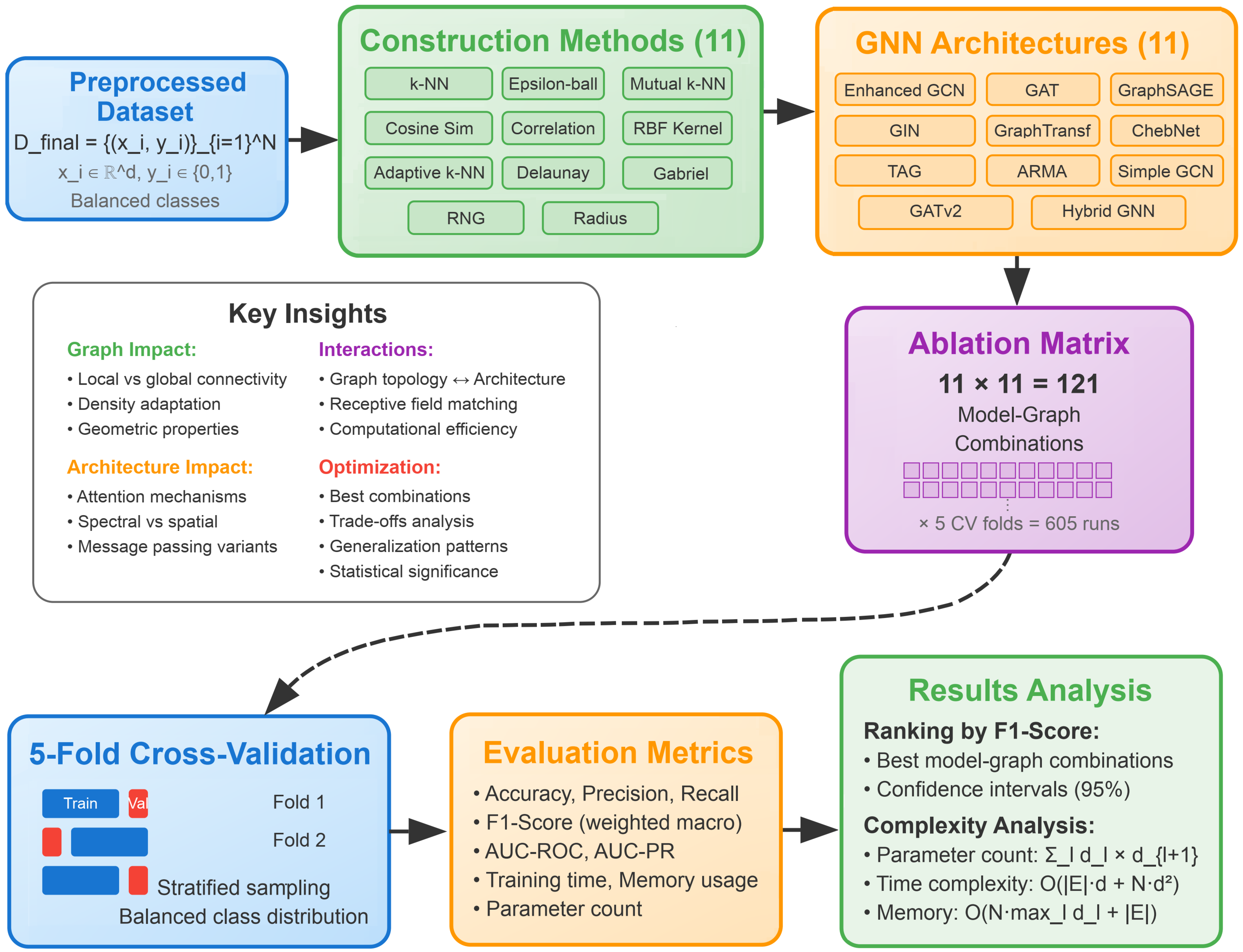
Figure 2 presents the complete pipeline of the ablation methodology applied in this paper. This comprehensive methodology ensures systematic evaluation of both graph construction strategies and GNN architectures while providing rigorous statistical analysis of performance differences across all experimental conditions. The large-scale ablation design enables identification of optimal model–graph combinations and provides insights into the interaction effects between graph topology and neural architecture choices.

The combination of 11 graph construction methods with 11 architectures results in 121 combinations that are compared in this study. To ensure robustness in the classification analysis and avoid bias, cross-validation is used. For cross-validation, a split of 80% of the data is considered for training and 20% for testing the model.

For each of the graphs, 23 samples were considered.

The proposed mathematical framework is broadly applicable to sensor-rich infrastructures; its development and validation within the context of NPPs are driven by the high-stakes, safety-critical, and sensor-dense nature of these facilities. Nowadays, studies have been increasingly presented to improve the design and safety of NPPs [55].

5. Results and Discussion

This section presents the results and discussions of the proposed method. We conducted 330 individual experiments across 11 GNN architectures and 11 graph construction methods using 3-fold stratified cross-validation.

For all evaluated experiments, we used synthetic data created using PCTRAN, having a total of 20 different simulated anomalies. For each of the experiments, 96 variables are recorded (see

Table A1. PCTRAN variables (1/2).

Description	Acronym
Activity reactor coolant (CPM)	RC87
Clad failure (%)	FRCL
Concentration reactor building hydrogen (%)	CNH2
Concentration reactor coolant I-131 (GBq/cc)	RC131
Concentration reactor coolant system boron (ppm)	PPM
Dose rate exclusion area boundary thyroid (mSv/h)	DTHY
Dose rate exclusion area boundary whole body (mSv/h)	DWB
Flow accumulator (t/h)	WCFT
Flow charging (t/h)	WCHG
Flow containment spray (t/h)	WCSP
Flow high pressure injection (t/h)	WHPI
Flow letdown (t/h)	WLD
Flow low-pressure injection (residual heat removal) (t/h)	WLPI
Flow pressurizer spray (t/h)	WSPY
Flow Przr power-operated relief valve and safeties (t/h)	WUP
Flow reactor coolant system leak (t/h)	WLR
Flow reactor coolant loop (t/h)	WRCA and WRCB
Flow steam generator feedwater (t/h)	WFWA and WFWB
Flow steam generator main steam (t/h)	WRLA and WRLB
Flow steam generator steam (t/h)	WSTA and WSTB
Flow steam generator tube leak (t/h)	WTRA and WTRB
Flow total break entering reactor building (t/h)	WBK
Flow total emergency core cooling system (t/h)	WECS
Fraction Zr oxidation	FRZR
Integrated break energy (MJ)	EBK
Integrated break flow (kg)	MBK
Level core water (m)	LVCR
Level pressurizer (%)	LVPZ
Level reactor building sump water (m)	LWRB
Level steam generator narrow range (%)	NSGA and NSGB
Level steam generator wide range (m)	LSGA and LSGB
Mass H2 generated by Zr-H2O (kg)	MH2
Mass of contingency cooling injection gases (kg)	MGAS
Mass of corium in DW (kg)	MDBR
Mass of molten concrete (kg)	MCRT
Mass total leakage out of reactor building (kg)	RBLK
Mass total leakage out of SGs (kg)	SGLK
Power core thermal (%)	PWR
Power fan cooler heat removal (MW)	QFCL
Power nuclear flux (%)	PWNT
Power pressurizer heater (kW)	HTR
Power residual heat removal rate (MW)	QRHR
Power steam generator heat removal (MW)	QMGA and QMGB
Power total megawatt thermal (MW)	QMWT
Power turbine load (%)	TBLD
Press partial reactor building air (bar)	PRBA
Press reactor building (bar)	PRB
Press reactor coolant system (bar)	P
Pressure steam generator (bar)	PSGA and PSGB
Rad monitor aux building air (CPM)	RM4

and

Table A2. PCTRAN variables (2/2).

Description	Acronym
Rad monitor condenser off-gas (CPM)	RM3
Rad monitor reactor building air (CPM)	RM1
Rad monitor steam line (CPM)	RM2
Rad rel rate condenser off-gas (GBq/s)	STTB
Rad rel rate reactor building (GBq/s)	STRB
Rad rel rate steam generator valves (GBq/s)	STSG
Ratio departure from nuclear boiling	DNBR
Reactivity fuel (doppler) (%dk/k)	RHFL
Reactivity mod temperature (%dk/k)	RHMT
Reactivity rod (%dk/k)	RHRD
Reactivity soluble boron (%dk/k)	RHBR
Reactivity total (%dk/k)	RH
Temp average fuel (°C)	TF
Temp hot leg (°C)	THA and THB
Temp loop subcooling margin (°C)	SCMA and SCMB
Temp of debris in cavity (°C)	TDBR
Temp of molten concrete (°C)	TCRT
Temp of debris in lower plenum (°C)	TSLP
Temp peak clad (°C)	TPCT
Temp peak fuel (°C)	TFPK
Temp Przr saturation (°C)	TSAT
Temp reactor building (°C)	TRB
Refueling water storage tank water volume (m3)	TKLV
Spec enthalpy Przr top discharge (kJ/kg)	HUP
Spec enthalpy reactor coolant system leak (kJ/kg)	HLW
Temp submerged fuel average (°C)	TFSB
Temperature cold leg (°C)	TCA and TCB
Temperature reactor coolant system average (°C)	TAVG
Volume reactor coolant system liquid (m3)	VOL
Void of reactor coolant system (%)	VOID

). These variables describe the physical, thermal–hydraulic, radiological, and reactivity-related conditions of a pressurized water reactor during normal operation and accident scenarios.

In this work, a pressurized water reactor with an inverted U-tube steam generator is considered (https://www.microsimtech.com/pctran/page2.htm (accessed on 21 December 2025)). For future evaluation, the simulated malfunctions are available at: https://github.com/SFStefenon/NPPmalfunctions (accessed on 21 December 2025).

5.1. Evaluation Metrics

The experimental evaluation was performed utilizing the foreblocks library (https://github.com/lseman/foreblocks (accessed on 21 December 2025)), an internally developed yet publicly accessible framework for time-series forecasting. The algorithms were written considering the Python language. For each model–graph combination, we compute comprehensive performance metrics across all folds to ensure robust statistical analysis. The classification accuracy, weighted precision, weighted recall, and weighted F1-Score are considered, given by

$$\begin{array}{c}\hfill \mathrm{Accuracy}={\displaystyle \frac{\left|\right\{i:arg{max}_c{\widehat{y}}_{ic}=arg{max}_c{y}_{ic}\left\}\right|}{N}}\end{array}$$

(32)

$$\begin{array}{c}\hfill {\mathrm{Prec}}_w=\sum _{c=1}^C{\displaystyle \frac{n_c}{N}}·{\displaystyle \frac{T{P}_c}{T{P}_c+F{P}_c}}\end{array}$$

(33)

where $n_c$ is the number of samples in class c, $T{P}_c$ is true positives, and $F{P}_c$ is false positives for class c.

$$\begin{array}{c}\hfill {\mathrm{Rec}}_w=\sum _{c=1}^C{\displaystyle \frac{n_c}{N}}·{\displaystyle \frac{T{P}_c}{T{P}_c+F{N}_c}}\end{array}$$

(34)

where $F{N}_c$ represents false negatives for class c.

$$\begin{array}{c}\hfill F{1}_w=\sum _{c=1}^C{\displaystyle \frac{n_c}{N}}·{\displaystyle \frac{2·{\mathrm{Prec}}_c·{\mathrm{Rec}}_c}{{\mathrm{Prec}}_c+{\mathrm{Rec}}_c}}.\end{array}$$

(35)

The macro-averaged metrics, unweighted averages across classes, are

$$\begin{array}{cc}\hfill {\mathrm{Prec}}_{\mathrm{macro}}& ={\displaystyle \frac{1}{C}}\sum _{c=1}^C{\mathrm{Prec}}_c\hfill \end{array}$$

(36)

$$\begin{array}{cc}\hfill {\mathrm{Rec}}_{\mathrm{macro}}& ={\displaystyle \frac{1}{C}}\sum _{c=1}^C{\mathrm{Rec}}_c\hfill \end{array}$$

(37)

$$\begin{array}{cc}\hfill F{1}_{\mathrm{macro}}& ={\displaystyle \frac{1}{C}}\sum _{c=1}^{C}F{1}_c\hfill \end{array}$$

(38)

The area under the receiver operating characteristic curve (AUC-ROC) for binary classification is given by

$$\begin{array}{c}\hfill \mathrm{AUC-ROC}={\int }_0^1\mathrm{TPR}\left({\mathrm{FPR}}^{-1}\left(x\right)\right)dx\end{array}$$

(39)

where TPR is the true positive rate and FPR is the false positive rate.

The area under the precision-recall curve (AUC-PR) is

$$\begin{array}{c}\hfill \mathrm{AUC-PR}={\int }_0^1\mathrm{Prec}\left(r\right)dr\end{array}$$

(40)

where precision is expressed as a function of recall r.

5.2. Experimental Configuration

The experimental framework employed a hybrid false positive generation method with class balancing through oversampling to address dataset imbalance. Models were trained for up to 50 epochs with early stopping mechanisms. The evaluation used 3-fold cross-validation across 330 total experiments, testing each architecture–method combination. The results represent means and standard deviations (StD) across all experiments.

Dataset preprocessing included synthetic false positive injection using hybrid noise patterns at 10% intensity, followed by oversampling-based class balancing. This configuration simulates operational conditions where threat detection systems encounter both genuine threats and false positives designed to evade detection.

5.3. GNN Architecture Performance

Table 2. Performance comparison of GNN architectures for threat detection.

Architecture	Accuracy		F1-Score		AUC-ROC		Time (s)
	Mean	StD	Mean	StD	Mean	StD	Mean	StD
GATv2	0.802	0.169	0.797	0.176	0.885	0.169	0.082	0.028
GraphSAGE	0.788	0.123	0.785	0.125	0.916	0.088	0.062	0.005
GraphTransformer	0.788	0.125	0.785	0.127	0.900	0.101	0.073	0.025
ChebNet	0.789	0.101	0.784	0.106	0.894	0.097	0.112	0.023
TAG-Conv	0.782	0.093	0.779	0.095	0.920	0.082	0.104	0.011

Best results in bold.

presents the performance comparison of GNN architectures averaged across all graph construction methods. GATv2 achieved the highest classification accuracy (0.802 ± 0.169) and F1-score (0.797 ± 0.176). GraphSAGE demonstrated the fastest training time (0.062 ± 0.005 s) while maintaining accuracy (0.788 ± 0.123).

TAG-Conv achieved the highest AUC-ROC score (0.920 ± 0.082). The attention-based architectures outperformed the convolution-based methods in classification metrics. GraphSAGE exhibited stable performance with low variance in training time, making it suitable for real-time deployment scenarios.

5.4. Graph Construction Method Performance

Table 3. Performance analysis of graph construction methods across all GNN architectures.

Method	Accuracy		F1-Score		AUC-ROC		Time (s)
	Mean	StD	Mean	StD	Mean	StD	Mean	StD
Mutual k-NN	0.838	0.080	0.835	0.082	0.920	0.095	0.077	0.024
Delaunay	0.811	0.102	0.808	0.105	0.910	0.091	0.090	0.031
Gabriel Graph	0.806	0.138	0.801	0.145	0.941	0.092	0.085	0.029
k-NN	0.801	0.095	0.798	0.099	0.906	0.098	0.090	0.024
Relative Neighbor.	0.793	0.102	0.788	0.105	0.907	0.089	0.078	0.028

Best results in bold.

shows the performance analysis of graph construction methods averaged across all GNN architectures. Mutual k-NN achieved the highest accuracy (0.838 ± 0.080) and F1-score (0.835 ± 0.082) while providing the fastest average training time (0.077 ± 0.024 s). Gabriel Graph achieved the highest AUC-ROC score (0.941 ± 0.092).

Proximity-based methods (Mutual k-NN, Gabriel Graph) outperformed similarity-based approaches, indicating that geometric relationships in feature space provide more informative connectivity patterns for threat detection. The standard deviations across methods demonstrate stable performance characteristics.

5.5. Architecture-Method Combinations

Table 4. Top 10 architecture–graph method combinations ranked by F1-score, including average training and inference time.

Architecture	Graph Method	Accuracy	F1-Score	AUC-ROC	Train Time (s)	Inference Time (s)
GAT	Mutual k-NN	0.884	0.882	0.979	0.070	0.00035
GAT	k-NN	0.880	0.880	0.921	0.094	0.00035
GATv2	Delaunay	0.880	0.880	0.900	0.103	0.00037
Simple GCN	Delaunay	0.880	0.880	0.904	0.053	0.00014
GATv2	Relative Neighborhood	0.880	0.874	0.979	0.064	0.00037
GraphTransformer	Gabriel Graph	0.875	0.873	0.938	0.095	0.00028
GraphSAGE	Mutual k-NN	0.847	0.845	0.871	0.063	0.00013
GraphTransformer	Mutual k-NN	0.847	0.845	0.829	0.086	0.00028
ChebNet	Mutual k-NN	0.847	0.845	0.946	0.111	0.00052
GIN	Delaunay	0.847	0.845	0.925	0.057	0.00014
Baseline Methods
MLP	–	0.760	0.722	0.900	–	–
SVM (RBF)	–	0.767	0.724	0.833	–	–
Random Forest	–	0.687	0.622	0.833	–	–

Best graph-based results in bold. Inference time reported as average per forward pass.

presents the top-performing architecture–method combinations ranked by F1-score. The GAT architecture with Mutual k-NN graph construction achieved the highest performance across all metrics, with an accuracy of 0.884, an F1-score of 0.882, and an AUC-ROC of 0.979. This combination (architecture with graph construction method) also maintained an efficient training time of 0.070 s.

The results show that attention-based architectures (GAT, GATv2) combined with proximity-based graph construction methods (Mutual k-NN, Delaunay) achieve superior performance. Simple GCN with Delaunay triangulation provides a computationally efficient alternative, achieving competitive accuracy (0.880) with the fastest training time (0.053 s).

5.6. Performance Analysis

The experimental results demonstrate performance differences between architectures and graph construction methods. Standard deviations across all metrics remain below 0.18, indicating stable performance characteristics. The performance differences between the top-performing combinations exceed two standard deviations.

Attention mechanisms provide advantages for threat detection, with GAT and GATv2 dominating the top combinations. However, computational efficiency considerations favor GraphSAGE and Simple GCN for real-time applications. The performance of the mutual k-NN and Delaunay methods across different architectures suggests that these graph construction approaches effectively capture threat-relevant structural patterns in the data.

5.6.1. Performance Distribution Analysis

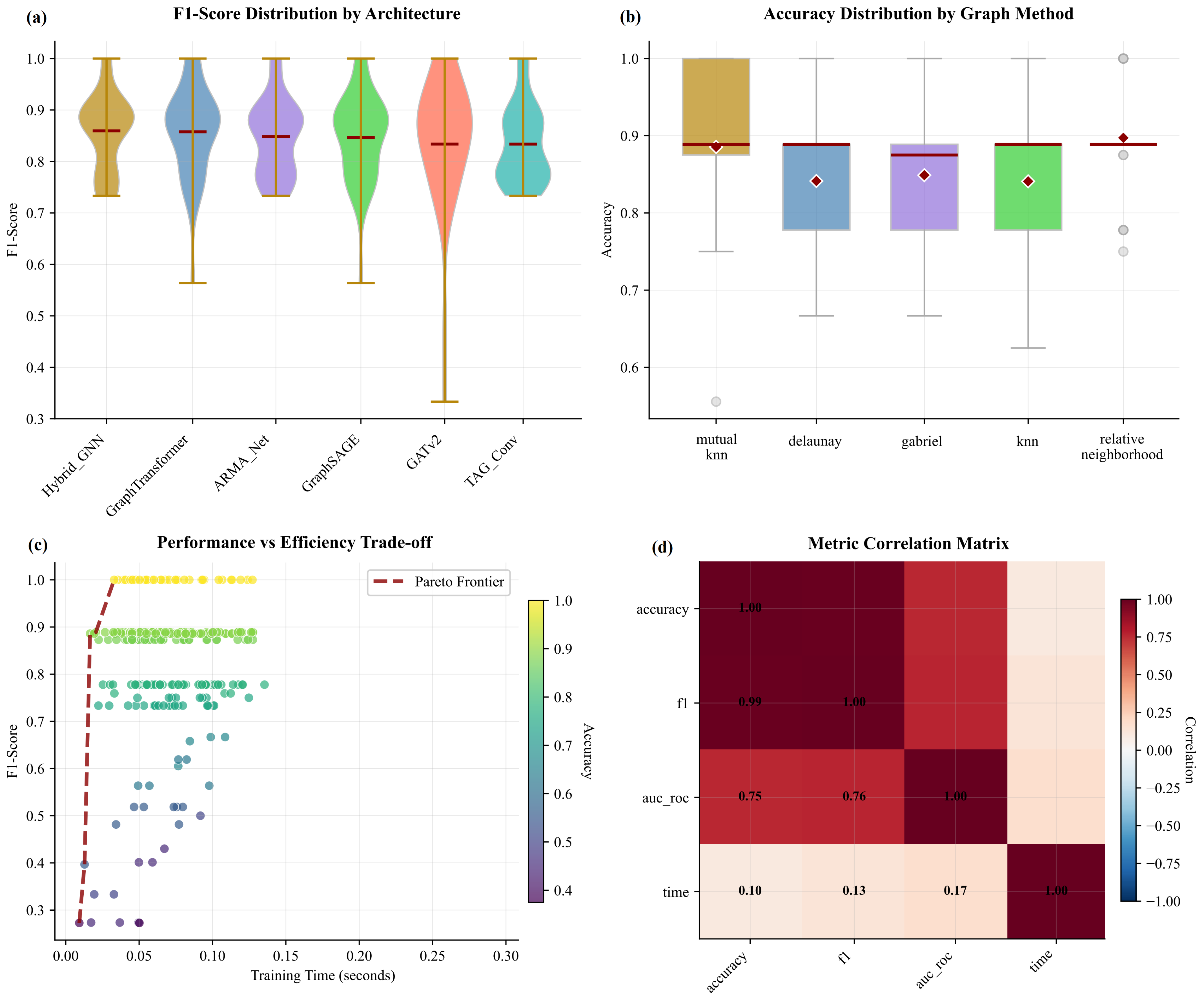
Figure 3 presents the performance distribution analysis across different architectures and graph construction methods. The violin plots in Figure 3a reveal that Hybrid GNN demonstrates the most consistent performance distribution with minimal variance, while GATv2 shows a broader distribution, indicating higher sensitivity to different graph configurations. TAG-Conv exhibits bimodal distribution patterns, suggesting performance depends heavily on specific graph construction methods. The differences in the mean F1-score between the architectures are subtle. The biggest differences are in the variability of the results, with some models showing poor performance in some of the experiments.

The box plots in Figure 3b show that mutual k-NN achieves the highest median accuracy (0.89) with the smallest interquartile range, indicating both high performance and stability. Gabriel’s graph construction shows the largest variance, with outliers extending below 0.75 accuracy. This result confirms that mutual k-NN is the best strategy to employ for the fault classification conducted here using graph-based architectures.

The Pareto frontier analysis in Figure 3c identifies optimal trade-offs between training time and F1-score. Points on the frontier represent architectures that cannot be improved in one metric without degrading the other. The vast majority of experiments showed that it is possible to achieve high accuracy values even in the short time used to train the model, with all experiments requiring less than 15 s for the model to be trained, considering the hardware characteristics used in this work. This shows that the models used require little computational effort and are capable of achieving high accuracy values.

The correlation matrix in Figure 3d reveals a strong positive correlation between accuracy and F1-score (r = 0.99), while training time shows a weak correlation with performance metrics (r = 0.10–0.17). Given the strong correlation between accuracy and F1-score, the model meets the expectations of projects focused on improving classification performance. In addition to the time required to train the model being acceptable, there is no correlation between training time and classification performance, which shows that the model is efficient, achieving satisfactory classification results in a short training time.

5.6.2. Statistical Significance Analysis

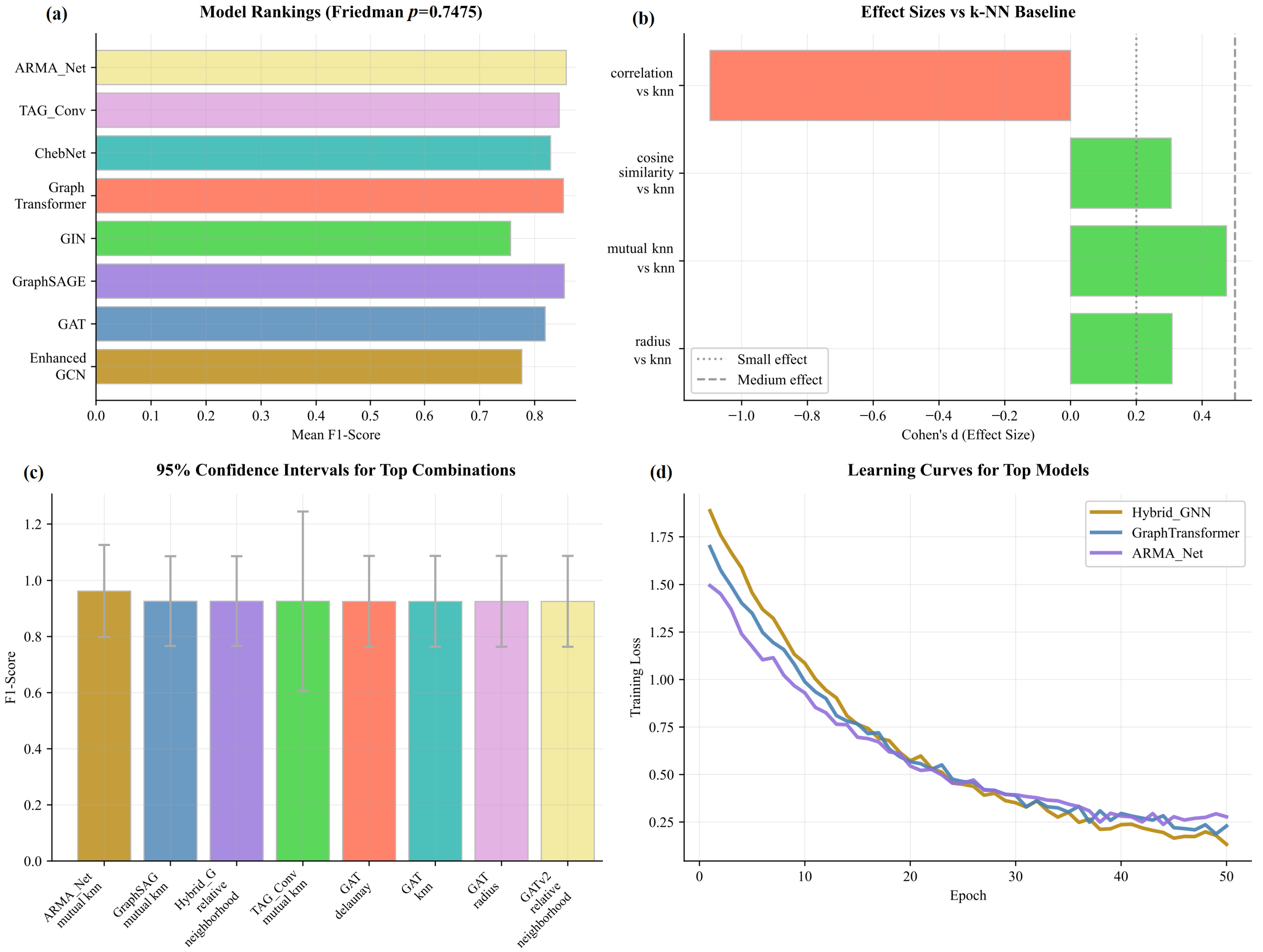
Figure 4 presents statistical tests and significance analysis. The Friedman test results in Figure 4a show no statistically significant differences between model architectures (p = 0.7475), indicating that architecture choice has less impact than graph construction method selection. In the Friedman test, p (p-value) tells the probability of observing the rank differences assuming the null hypothesis is true.

Effect size analysis in Figure 4b demonstrates that mutual k-NN and cosine similarity methods show medium effect sizes (Cohen’s d > 0.2) compared to the standard k-NN baseline. Correlation-based graph construction shows a negative effect size, indicating inferior performance relative to k-NN. The confidence interval analysis in Figure 4c reveals that GAT with mutual k-NN achieves the highest performance (F1 = 0.96) with tight confidence bounds. The learning curves in Figure 4d show that Hybrid GNN converges fastest, reaching stable performance within 15 epochs, while GraphTransformer requires 25–30 epochs for convergence.

5.6.3. Graph Topology Impact Analysis

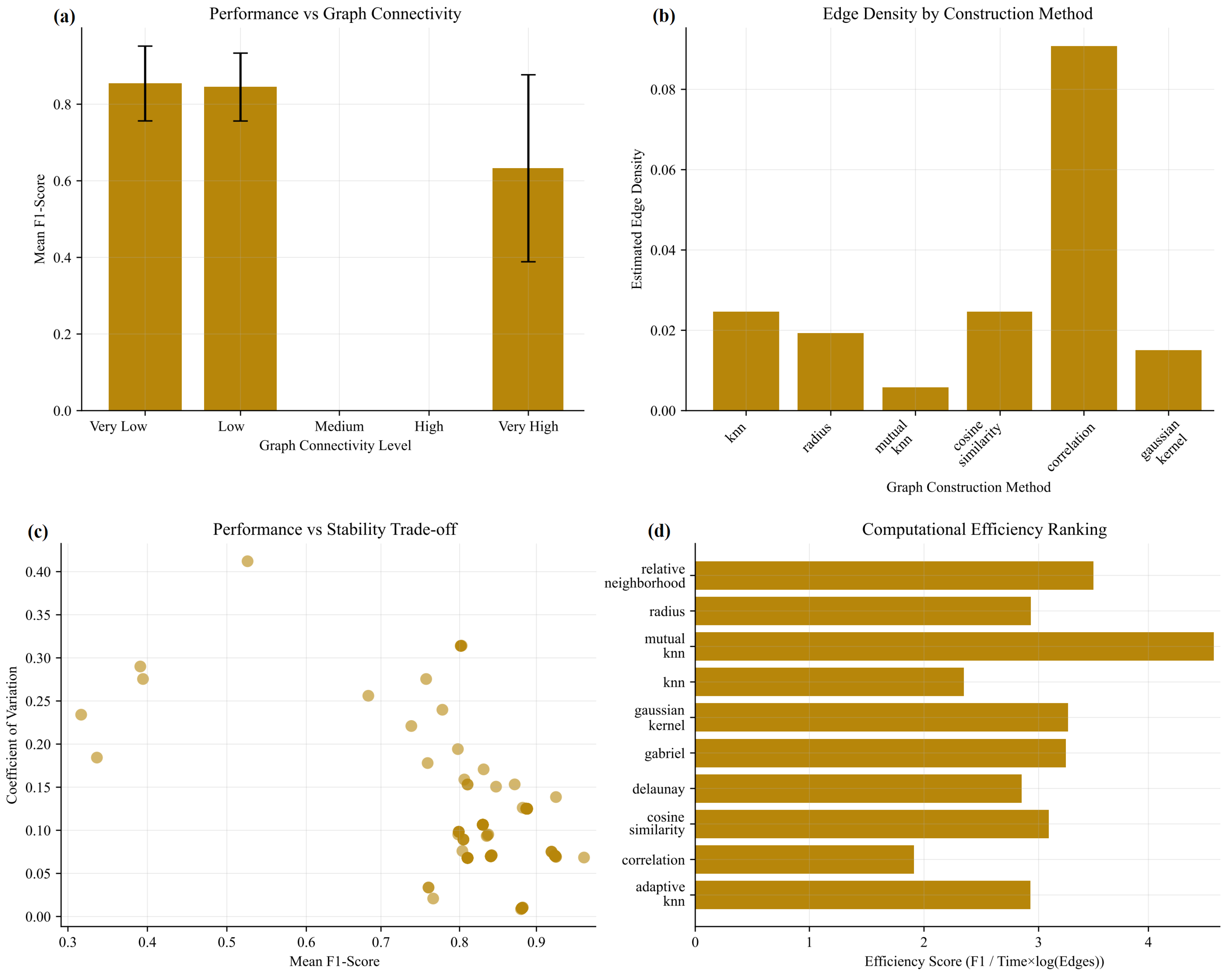
Figure 5 examines the relationship between graph topology and performance. The connectivity analysis in Figure 5a shows that very low and low connectivity levels achieve the highest mean F1-scores (0.82–0.83), while medium to very high connectivity degrades performance. This suggests that sparse, well-connected graphs are optimal for threat detection tasks.

Edge density comparison in Figure 5b reveals that correlation-based methods produce the densest graphs, while mutual k-NN maintains moderate density. The performance vs. stability trade-off in Figure 5c identifies combinations with both high performance and a low coefficient of variation, with GAT-mutual k-NN achieving the optimal balance.

The computational efficiency ranking in Figure 5d shows mutual k-NN as the most efficient method, achieving a high F1-score per unit of computational cost. Relative neighborhood and radius methods also demonstrate good efficiency, while adaptive k-NN shows the lowest efficiency, despite its competitive performance.

5.6.4. Detailed Performance Analysis

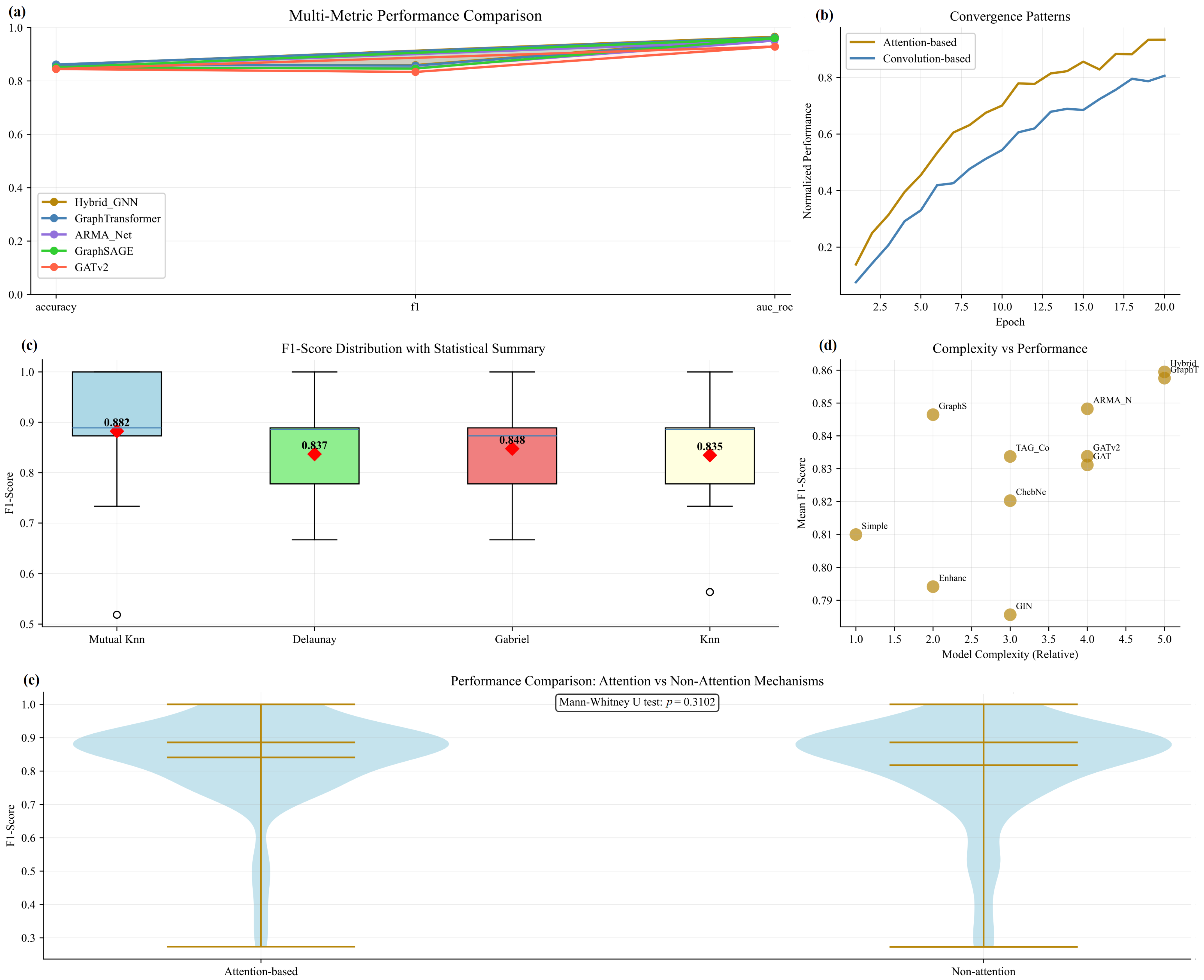
Figure 6 provides multi-dimensional performance analysis. The radar chart in Figure 6a shows that GATv2 achieves balanced performance across all metrics, while GraphSAGE excels in AUC-ROC but shows a lower accuracy and F1-score. Hybrid GNN demonstrates the most balanced profile across accuracy, F1-score, and AUC-ROC.

Convergence pattern analysis in Figure 6b reveals that attention-based models converge faster and achieve higher asymptotic performance compared to convolution-based approaches. The attention mechanism comparison in Figure 6e shows no statistically significant difference between attention-based and non-attention models (p = 0.3102), though attention-based models demonstrate slightly higher median performance.

For the Mann–Whitney U test, p (p-value) is the probability of obtaining a difference between the two groups as extreme as the observed one, assuming that the null hypothesis is true The complexity vs. performance analysis in Figure 6d indicates that model complexity does not strongly correlate with performance. Simple GCN achieves competitive results with low complexity, while more complex models like Hybrid GNN and GraphTransformer show marginal performance gains.

5.7. Physical Explanation for Best Performance

Mutual k-NN produced the best results because its graph topology aligns more closely with the physical coupling principles that govern NPP sensor behavior. In a thermodynamic system, two sensors influence one another only when they share a genuine physical coupling such as mass-flow continuity, energy balance, pressure–temperature interdependence, or spatial adjacency in a hydraulic loop. Mutual k-NN preserves these strong, reciprocal relationships by creating edges only when the sensor is among the closest neighbors. This reciprocity filters out statistical similarities that frequently appear in correlation-based graphs, where high correlations may arise from global trends, transient common-mode effects, or indirect dependencies rather than true physical interactions.

Mutual k-NN produces a sparse but physically faithful graph in which edges reflect only robust thermodynamic couplings, such as the paired behavior of temperature and pressure sensors in the primary circuit, or feedwater and steam sensors in the secondary loop. This structure allows the GAT layers to propagate information along paths that correspond to real heat-transfer and fluid-flow mechanisms, improving anomaly localization and preventing error propagation through irrelevant or non-physical links. Consequently, the model trained on mutual k-NN can distinguish genuine fault propagation from isolated sensor anomalies with greater precision, which explains its superior performance in this thermodynamic context.

5.8. Comparison with Other Research

While the results are derived from a controlled, synthetic dataset, they support the core conclusion that the proposed GAT-Mk-NN framework represents a promising approach for predictive maintenance in NPPs. The comprehensive ablation study, encompassing several model–graph combinations, provides statistically significant evidence that the mutual k-NN graph construction combined with an attention-based GNN architecture achieves the optimal trade-off between accuracy (0.884), F1-score (0.882), and computational efficiency for fault discrimination.

Several studies focused on NPPs applied standard models without extensive comparisons of possible combinations for solving tasks in this field [15,16]. Our work presents a comparison approach with several structures and methods to create an efficient model for classifying failures in NPPs. In [17], the authors achieved 99.20% accuracy, with Petri Net proving to be a very promising solution for fault classification.

New techniques have been applied, successfully combining state-of-the-art models for fault classification in NPPs, such as the work by Wang et al. [18], which uses a combination of FFT, LSTM, and GCN. In Jyotish et al. [20], using a reachability graph and ordinary differential equations, the authors achieved an accuracy of 99.5%. In fact, the use of graphs has been more widely applied in the literature with promising results, motivating the complete evaluation of the structures, as presented in this paper.

5.9. Operational Implementation Example

To demonstrate the practical application of the developed GAT-Mk-NN method, consider a real-world diagnostic scenario in a pressurized water reactor NPP. During operation, a temperature sensor (e.g., hot leg temperature) begins reporting anomalous readings that suggest a rapid rise in primary coolant temperature, a potential indicator of a loss-of-coolant accident. In a traditional monitoring system, this could trigger an unnecessary shutdown or alarm flood. However, the deployed GAT-Mk-NN model evaluates this reading within the context of its graph neighborhood, which includes physically linked sensors such as pressure, cold leg temperature, steam generator pressure, and reactor power.

The attention mechanism weights the information from these neighboring nodes and detects that, while the temperature hot leg shows an outlier, the correlated readings from pressure and flow sensors remain within normal operational bounds, and no complementary spike in containment radiation or building pressure is observed. The model therefore classifies the anomaly as a sensor-level false positive, likely due to drift or calibration error, rather than a system-level fault. This allows operators to schedule targeted sensor maintenance without disrupting plant operation, thereby enhancing diagnostic accuracy, reducing false alarms, and supporting predictive maintenance decisions in real time.

6. Conclusions

This work presented a framework for improving predictive maintenance in NPPs by combining false positive generation, dataset balancing, and GNN ablation analysis. Synthetic anomalies were generated using structured perturbation strategies and integrated into the training set through controlled oversampling, aiming to expose models to realistic misclassification scenarios.

Ablation experiments across multiple GNN architectures and graph construction methods showed that proximity-based graphs, such as mutual k-NN and Delaunay triangulation, consistently yielded better classification performance. Among the considered models, attention-based architectures, particularly GAT combined with mutual k-NN, achieved the highest accuracy and F1-scores. The analysis also showed that sparse graphs with moderate connectivity often provided a good balance between expressiveness and training efficiency.

This study further examined training stability, learning dynamics, and performance-efficiency trade-offs, supporting informed model selection depending on available computational resources and application constraints. These results provide a basis for applying graph-based learning to fault detection in sensor-rich industrial environments.

Future extensions may include multi-fault modeling, temporal graph representations, and causal inference techniques to improve diagnostic coverage and adaptability under changing operating conditions. To facilitate the deployment of the GAT-Mk-NN in operational nuclear power plants, several practical measures can be adopted. For edge computing constraints, the model can be optimized to reduce computational and memory footprints, enabling execution on local sensor nodes or gateway devices with minimal latency.

To meet nuclear regulators’ requirements for explainability, attention weights from the GAT layers can be visualized to highlight influential sensor relationships, and rule-extraction techniques can be employed to generate human-interpretable diagnostic logs. Integration with existing SCADA (Supervisory Control and Data Acquisition) systems can be achieved through modular APIs or middleware that translate model outputs into standardized alarms and advisories, ensuring compatibility with real-time monitoring interfaces and preserving existing operational workflows.

To further strengthen the validation and applicability of the GAT-Mk-NN, future work could incorporate cross-dataset evaluation using publicly available NPP fault datasets or data from different reactor types to assess generalization.

References

1. Yin, W.; Zhu, S.; Xia, H. Fault detection for time-varying process in nuclear power plants based on improved moving window and dynamic kernel principal component analysis. Reliab. Eng. Syst. Saf. 2025, 264, 111441. [Google Scholar] [CrossRef]
2. Wang, H.; Peng, M.J.; Yu, Y.; Saeed, H.; Hao, C.M.; Liu, Y.K. Fault identification and diagnosis based on KPCA and similarity clustering for nuclear power plants. Ann. Nucl. Energy 2021, 150, 107786. [Google Scholar] [CrossRef]
3. Liu, B.; Lei, J.; Xie, J.; Zhou, J. Development and validation of a nuclear power plant fault diagnosis system based on deep learning. Energies 2022, 15, 8629. [Google Scholar] [CrossRef]
4. Lin, T.H.; Wang, T.C.; Wu, S.C. Deep learning schemes for event identification and signal reconstruction in nuclear power plants with sensor faults. Ann. Nucl. Energy 2021, 154, 108113. [Google Scholar] [CrossRef]
5. Chen, E.; Bao, H.; Dinh, N. Evaluating the reliability of machine-learning-based predictions used in nuclear power plant instrumentation and control systems. Reliab. Eng. Syst. Saf. 2024, 250, 110266. [Google Scholar] [CrossRef]
6. Yin, W.; Xia, H.; Wang, Z.; Yang, B.; Zhang, J.; Jiang, Y.; Miyombo, M.E. A fault diagnosis of nuclear power plant rotating machinery based on multi-sensor and deep residual neural network. Ann. Nucl. Energy 2023, 185, 109700. [Google Scholar] [CrossRef]
7. Seman, L.O.; Aquino, L.S.; Stefenon, S.F.; Yow, K.C.; Mariani, V.C.; dos Santos Coelho, L. Simultaneously anomaly detection and forecasting for predictive maintenance using a zero-cost differentiable architecture search-based network. Comput. Ind. Eng. 2025, 208, 111412. [Google Scholar] [CrossRef]
8. Choi, J.; Lee, S.J. RNN-based integrated system for real-time sensor fault detection and fault-informed accident diagnosis in nuclear power plant accidents. Nucl. Eng. Technol. 2023, 55, 814–826. [Google Scholar] [CrossRef]
9. Zhu, S.; Xia, H.; Annor-Nyarko, M.; Yin, W.; Peng, B.; Wang, Z.; Zhang, J. A robust strategy for sensor fault detection in nuclear power plants based on principal component analysis. Ann. Nucl. Energy 2021, 164, 108621. [Google Scholar] [CrossRef]
10. Zheng, Q.; Lu, L.; Sun, F.; Chen, Z.; Wu, Q.; Hou, B.; Yang, J.; Zhu, H.; Yang, L.; Wang, Y.; et al. Deep learning-driven thermal conductivity evaluation of aerogel composite felt for nuclear power pipelines insulation. Sustain. Mater. Technol. 2025, 46, e01729. [Google Scholar] [CrossRef]
11. Zhang, S.; Ma, X.; Nie, Z.; Cheng, W.; Xing, J.; Zhang, L.; Hong, J.; Xu, Z.; Chen, X. Integration of multi-relational graph oriented fault diagnosis method for nuclear power circulating water pumps. Measurement 2025, 242, 115811. [Google Scholar] [CrossRef]
12. Qu, Y.; Xue, X.; Shi, Y. Graph classification based fault detection in nuclear power plants with graph formulation. Procedia Comput. Sci. 2023, 221, 657–663. [Google Scholar] [CrossRef]
13. Wang, Y.; Cheng, Y.; Qi, Q.; Tao, F. IDS-KG: An industrial dataspace-based knowledge graph construction approach for smart maintenance. J. Ind. Inf. Integr. 2024, 38, 100566. [Google Scholar] [CrossRef]
14. Mamdikar, M.R.; Kumar, V.; Singh, P. Dynamic reliability analysis framework using fault tree and dynamic Bayesian network: A case study of NPP. Nucl. Eng. Technol. 2022, 54, 1213–1220. [Google Scholar] [CrossRef]
15. Li, M.; Xu, Z.; Yang, J.; Yang, M. A graph representation model for radiation exposure prediction and path-planning in nuclear power plants. Ann. Nucl. Energy 2021, 156, 108196. [Google Scholar] [CrossRef]
16. Wang, X.; Wang, H.; Peng, M. Interpretability study of a typical fault diagnosis model for nuclear power plant primary circuit based on a graph neural network. Reliab. Eng. Syst. Saf. 2025, 261, 111151. [Google Scholar] [CrossRef]
17. Jyotish, N.K.; Singh, L.K.; Kumar, C. Availability analysis of safety-critical systems of nuclear power plant using ordinary differential equations and reachability graph. Prog. Nucl. Energy 2023, 159, 104624. [Google Scholar] [CrossRef]
18. Wang, Y.; Liu, J.; Qian, G. Hierarchical FFT-LSTM-GCN based model for nuclear power plant fault diagnosis considering spatio-temporal features fusion. Prog. Nucl. Energy 2024, 171, 105178. [Google Scholar] [CrossRef]
19. Zhang, L.; Cheng, W.; Zhang, S.; Xing, J.; Chen, X.; Gao, L.; Xu, Z.; Yang, R.; Hong, J.; Ma, Y. Spatial-Temporal Graph Conditionalized Normalizing Flows for Nuclear Power Plant Multivariate Anomaly Detection. IEEE Trans. Ind. Inform. 2024, 20, 12945–12957. [Google Scholar] [CrossRef]
20. Jyotish, N.K.; Singh, L.K.; Kumar, C. Reliability assessment of safety-critical systems of nuclear power plant using ordinary differential equations and reachability graph. Nucl. Eng. Des. 2023, 412, 112469. [Google Scholar] [CrossRef]
21. Liu, S.; Zhou, X.; Yu, J.; Wang, Y.; Xu, T.; Wang, H. Graph attention Network-Based model for multiple fault detection and identification of sensors in nuclear power plant. Nucl. Eng. Des. 2024, 419, 112949. [Google Scholar] [CrossRef]
22. Chae, Y.H.; Lee, C.; Han, S.M.; Seong, P.H. Graph neural network based multiple accident diagnosis in nuclear power plants: Data optimization to represent the system configuration. Nucl. Eng. Technol. 2022, 54, 2859–2870. [Google Scholar] [CrossRef]
23. Fei, Z.; Manning, C.; West, G.M.; Murray, P.; Dobie, G. Enhanced video-level anomaly feature detection for nuclear power plant component inspections using the latency mechanism. Nucl. Technol. 2024, 210, 2404–2418. [Google Scholar] [CrossRef]
24. Dong, C.; Zhou, J. A New Algorithm of Cubic Dynamic Uncertain Causality Graph for Speeding Up Temporal Causality Inference in Fault Diagnosis. IEEE Trans. Reliab. 2023, 72, 662–677. [Google Scholar] [CrossRef]
25. Aminov, R.; Garievskii, M.; Anoshin, D. Development of design solutions for a latent heat thermal energy storage under conditions of its operation in a single energy complex with an NPP. Therm. Eng. 2024, 71, 203–214. [Google Scholar] [CrossRef]
26. Wu, G.; Yuan, D.; Yin, J.; Xiao, Y.; Ji, D. A framework for monitoring and fault diagnosis in nuclear power plants based on signed directed graph methods. Front. Energy Res. 2021, 9, 641545. [Google Scholar] [CrossRef]
27. Zhang, L.; Cheng, W.; Xing, J.; Chen, X.; Nie, Z.; Zhang, S.; Hong, J.; Xu, Z. Self-Supervised Variational Graph Autoencoder for System-Level Anomaly Detection. IEEE Trans. Instrum. Meas. 2023, 72, 3535111. [Google Scholar] [CrossRef]
28. Wang, Q.; Han, B. Temporal transaction network anomaly detection for Industrial Internet of Things with federated graph neural networks. Comput. Ind. Eng. 2025, 205, 111122. [Google Scholar] [CrossRef]
29. Westarb, G.; Stefenon, S.F.; Hoppe, A.F.; Sartori, A.; Klaar, A.C.R.; Leithardt, V.R.Q. Complex graph neural networks for medication interaction verification. J. Intell. Fuzzy Syst. 2023, 44, 10383–10395. [Google Scholar] [CrossRef]
30. Yamaguchi, C.K.; Stefenon, S.F.; Santana, J.F.D.P.; Leithardt, V.R.Q. Are Graph Neural Networks Better than Standard Classifiers? In Proceedings of the International Conference on Disruptive Technologies, Tech Ethics and Artificial Intelligence, Salamanca, Spain, 8–10 July 2025; Volume 5, pp. 36–47. [Google Scholar] [CrossRef]
31. Zhao, W.L.; Wang, H.; Ngo, C.W. Approximate k-NN Graph Construction: A Generic Online Approach. IEEE Trans. Multimed. 2022, 24, 1909–1921. [Google Scholar] [CrossRef]
32. Li, Q.; Wang, Y.; Chen, W.; Li, L.; Hao, H. Machine learning prediction of BLEVE loading with graph neural networks. Reliab. Eng. Syst. Saf. 2024, 241, 109639. [Google Scholar] [CrossRef]
33. Jiang, W.; Ning, B.; Li, G.; Bai, M.; Jia, X.; Wei, F. Graph-decomposed k-NN searching algorithm on road network. Front. Comput. Sci. 2024, 18, 183609. [Google Scholar] [CrossRef]
34. Calder, J.; Trillos, N.G. Improved spectral convergence rates for graph Laplacians on ε-graphs and k-NN graphs. Appl. Comput. Harmon. Anal. 2022, 60, 123–175. [Google Scholar] [CrossRef]
35. Susskind, L.; Susskind, L. Graph Theory Perspective. Three Lect. Complex. Black Holes 2020, 1, 21–29. [Google Scholar] [CrossRef]
36. Wang, L.; Luo, J.; Deng, S.; Guo, X. RoCS: Knowledge graph embedding based on joint cosine similarity. Electronics 2023, 13, 147. [Google Scholar] [CrossRef]
37. Vijayvargiya, A.; Kumar, R.; Sharma, P. PC-GNN: Pearson Correlation-Based Graph Neural Network for Recognition of Human Lower Limb Activity Using sEMG Signal. IEEE Trans. Hum.-Mach. Syst. 2023, 53, 945–954. [Google Scholar] [CrossRef]
38. Deng, Z.; Wang, J. G2-SCANN: Gaussian-kernel graph-based SLD clustering algorithm with natural neighbourhood. Pattern Recognit. 2024, 155, 110682. [Google Scholar] [CrossRef]
39. Yan, Y.; Zhou, T.; Zheng, Z.; Ge, H.; Zhang, Y.; Zhang, Y. Robust gravitation based adaptive k-NN graph under class-imbalanced scenarios. Knowl.-Based Syst. 2022, 239, 108002. [Google Scholar] [CrossRef]
40. Wang, P.; Wang, Z.; Xin, S.; Gao, X.; Wang, W.; Tu, C. Restricted delaunay triangulation for explicit surface reconstruction. ACM Trans. Graph. 2022, 41, 1–20. [Google Scholar] [CrossRef]
41. Jurkiewicz, P. TopoHub: A repository of reference Gabriel graph and real-world topologies for networking research. SoftwareX 2023, 24, 101540. [Google Scholar] [CrossRef]
42. Foster, C.; Sevilmis, B.; Kimia, B. Generalized relative neighborhood graph (GRNG) for similarity search. Pattern Recognit. Lett. 2025, 188, 103–110. [Google Scholar] [CrossRef]
43. Zhou, S.; Zhang, Y. Signless Laplacian spectral radius for a k-extendable graph. Filomat 2025, 39, 649–657. [Google Scholar] [CrossRef]
44. Starke, L.; Hoppe, A.F.; Sartori, A.; Stefenon, S.F.; Santana, J.F.D.P.; Leithardt, V.R.Q. Interference recommendation for the pump sizing process in progressive cavity pumps using graph neural networks. Sci. Rep. 2023, 13, 16884. [Google Scholar] [CrossRef]
45. Liang, B.; Su, H.; Gui, L.; Cambria, E.; Xu, R. Aspect-based sentiment analysis via affective knowledge enhanced graph convolutional networks. Knowl.-Based Syst. 2022, 235, 107643. [Google Scholar] [CrossRef]
46. Sun, Q.; Wei, X.; Yang, X. GraphSAGE with deep reinforcement learning for financial portfolio optimization. Expert Syst. Appl. 2024, 238, 122027. [Google Scholar] [CrossRef]
47. Wu, C.; Lou, Y.; Li, J.; Wang, L.; Xie, S.; Chen, G. A Multitask Network Robustness Analysis System Based on the Graph Isomorphism Network. IEEE Trans. Cybern. 2024, 54, 6630–6642. [Google Scholar] [CrossRef] [PubMed]
48. Chen, C.; Wu, Y.; Dai, Q.; Zhou, H.Y.; Xu, M.; Yang, S.; Han, X.; Yu, Y. A Survey on Graph Neural Networks and Graph Transformers in Computer Vision: A Task-Oriented Perspective. IEEE Trans. Pattern Anal. Mach. Intell. 2024, 46, 10297–10318. [Google Scholar] [CrossRef]
49. Tseng, C.C.; Lee, S.L. Minimax Design of Graph Filter Using Chebyshev Polynomial Approximation. IEEE Trans. Circuits Syst. II Express Briefs 2021, 68, 1630–1634. [Google Scholar] [CrossRef]
50. Du, J.; Zhang, S.; Wu, G.; Moura, J.M.; Kar, S. Topology adaptive graph convolutional networks. arXiv 2017, arXiv:1710.10370. [Google Scholar] [CrossRef]
51. Wang, Z.; Fu, L.; Ma, M.; Zhai, Z.; Chen, H. Extended ARMA graph neural networks for the prognosis of complex systems. Knowl.-Based Syst. 2025, 309, 112762. [Google Scholar] [CrossRef]
52. Wu, F.; Souza, A.; Zhang, T.; Fifty, C.; Yu, T.; Weinberger, K. Simplifying Graph Convolutional Networks. In Proceedings of the Machine Learning Research, Proceedings of the 36th International Conference on Machine Learning, Long Beach, CA, USA, 9–15 June 2019; ML Research Press: Cambridge, MA, USA, 2019; Volume 97, pp. 6861–6871. [Google Scholar]
53. Zhu, P.; Yuan, Y.; Chen, L. Electra-based graph network model for multi-hop question answering. J. Intell. Inf. Syst. 2023, 61, 819–834. [Google Scholar] [CrossRef]
54. Pfeifer, B.; Chereda, H.; Martin, R.; Saranti, A.; Clemens, S.; Hauschild, A.C.; Beißbarth, T.; Holzinger, A.; Heider, D. Ensemble-GNN: Federated ensemble learning with graph neural networks for disease module discovery and classification. Bioinformatics 2023, 39, btad703. [Google Scholar] [CrossRef] [PubMed]
55. Janczyszyn, J.; Domańska, G.; Oettingen, M. Simulation of the measured reactivity distributions in the subcritical MYRRHA reactor. Energies 2024, 17, 2565. [Google Scholar] [CrossRef]
Figure 1. Methodology for creating false positive samples.
Technologies 14 00026 g001
Figure 2. Pipeline of the ablation methodology.
Technologies 14 00026 g002
Figure 3. Performance distribution analysis showing (a) F1-score distribution by architecture using violin plots, (b) accuracy distribution by graph method with box plots and mean markers, (c) performance vs. efficiency trade-off with Pareto frontier, and (d) correlation matrix of evaluation metrics.
Technologies 14 00026 g003
Figure 4. Statistical significance analysis including (a) Friedman test rankings of model architectures, (b) Cohen’s d effect sizes compared to the k-NN baseline, (c) 95% confidence intervals for the top-performing combinations, and (d) learning curves showing convergence patterns for top models.
Technologies 14 00026 g004
Figure 5. Graph topology impact analysis showing (a) performance vs. graph connectivity levels, (b) edge density distribution by construction method, (c) a performance–stability trade-off scatterplot with the coefficient of variation, and (d) computational efficiency ranking based on F1-score normalized by time and graph complexity.
Technologies 14 00026 g005
Figure 6. Advanced performance analysis including (a) multi-metric radar chart comparison, (b) convergence patterns for attention vs. convolution-based models, (c) F1-score distribution with statistical summaries, (d) model complexity vs. performance scatterplot, and (e) violin plot comparison of attention vs. non-attention mechanisms with Mann–Whitney U test results.
Technologies 14 00026 g006