Dynamic Modeling and Analysis of Epidemic Spread Driven by Human Mobility

Abstract

A spatiotemporal transmission epidemic model is proposed based on human mobility, spatial factors of population migration across multiple regions, individual protection, and government quarantine measures. First, the model’s basic reproduction number and disease-free equilibrium are derived, and the relationship between the basic reproduction number in a single region and that across multiple regions is explored. Second, the global asymptotic stability of both the disease-free equilibrium and the endemic equilibrium is proved by constructing a Lyapunov function. The impact of population migration on the spread of the virus is revealed by numerical simulations, and the global sensitivity of the model parameters is analyzed for a single region. Finally, a protection isolation strategy based on the optimal path is proposed. The experimental results indicate that increasing the isolation rate, improving the treatment rate, enhancing personal protection, and reducing the infection rate can effectively prevent and control the spread of the epidemic. Population migration accelerates the spread of the virus from high-infected areas to low-infected areas, aggravating the epidemic situation. However, effective public health measures in low-infected areas can prevent transmission and reduce the basic reproduction number. Furthermore, if the inflow migration rate exceeds the outflow rate, the number of infected individuals in the region increases.

1. Introduction

Infectious diseases continue to pose threats to public health and social stability, disrupting social and economic order and daily life patterns [1]. In recent years, a variety of infectious diseases have emerged across different regions and countries, such as the COVID-19 pandemic [2,3], Ebola [4], HIV [5], and Dengue [6]. In the context of globalization, international travel and trade have accelerated cross-border population mobility. This connectivity enables infectious diseases to spread rapidly from localized outbreaks to a global scale. The dense urban environment and crowded public places have increased the frequency of interpersonal contact, further facilitating the spread of diseases. The transmission dynamics of infectious diseases are an inherently nonlinear process, which is influenced by complex factors such as vaccination, government intervention, and human mobility [7]. The large-scale human mobility plays a decisive role in enabling spatial dissemination, as it physically bridges outbreaks across regions. The spatiotemporal heterogeneity caused by large-scale human mobility determines the velocity and geographic reach of epidemics. Quantifying the mobility-driven mode of transmission not only improves predictive accuracy but also formulates intervention strategies. Thus, an effective epidemiological model should account for both localized outbreaks and cross-regional disease spread driven by large-scale human mobility.

However, existing single-region transmission models often fail to capture the impact of dynamic population mobility on interregional disease spread, particularly in a highly interconnected world [8]. While these transmission models can effectively characterize the evolutionary mechanisms of local epidemics, they struggle to incorporate the complex, real-time effects of human movement across regions, which are critical drivers of disease spread in a globalized context.

To address these limitations, we propose a nonlinear dynamic model that considers three critical factors: multi-regional population migration, low-risk population, and isolated population. The primary contributions of this paper are described as follows:

(1)

According to the transmission characteristics of infectious diseases, a multi-regional spatio-temporal transmission dynamic model is proposed, considering low-risk population, isolation factors, and population flow between different regions.

(2)

We calculate the basic reproduction number, and the relationship between the basic reproduction number of a single region and that of multiple regions is explored. Furthermore, the global stability of the model’s equilibrium points is proved by constructing a Lyapunov function.

(3)

The impact of population mobility on the transmission of infectious diseases is studied. Latin hypercube sampling (LHS) and partial rank correlation coefficient (PRCC) are used to analyze the global parameter sensitivity in a single region. A protective isolation strategy is designed on the basis of the optimal path.

The structure of this paper is organized as follows: Section 2 reviews related works. The SLEIQDR model of multi-regional population migration based on the SEIR model is described in Section 3. Section 4 analyzes the global stability of the disease-free equilibrium and the endemic equilibrium of the model. In Section 5, the theories in Section 4 are proved by numerical simulations, and the model’s parameter effects on infectious diseases are analyzed through global sensitivity analysis. Finally, Section 6 summarizes the work of this paper.

2. Related Works

At present, the most representative dynamic models of infectious disease include the susceptible-infected-recovered (SIR) model, the susceptible-infected-recovered-susceptible (SIRS) model, and the susceptible-exposed-infected-recovered (SEIR) model. These dynamic models are based on nonlinear dynamics theory and aim to explore the virus’s evolution, transmission mechanisms, and predict the epidemic’s future trajectory. Alkhazzan et al. [9] propose a new stochastic SIRS model and analyze the dynamics of two diseases simultaneously. The model includes media coverage, treatment functions, and three types of noise factors. Ishtiaq et al. [10] propose a delayed stochastic SIRS model that incorporates an exponential birth rate and a saturated incidence function and analyze its dynamics. Yin et al. [11] integrate the SIR model with multilayer networks and study the joint dynamics of information and epidemics spread across different networks influenced by government policies. Centres et al. [12] integrate the SIR Model with mobile agent diffusion characteristics and propose two infectious mechanisms–direct contact and close transmission–to simulate disease spread more accurately. Song et al. [13] combine asynchronous state estimation with a nonlinear reaction-diffusion SIR Model to solve the shortcomings of existing models in multi-stage epidemic propagation modeling and state estimation. Khalifi et al. [14] introduce the heterogeneity of individual immunity into the SIRS model, which can predict the spread trend of the epidemic more accurately. Guan et al. [15] use rubella as an example to study a network-based SIR epidemic model that combines saturation infectivity, vertical transmission, and pulse vaccination strategies. The dynamic behavior of the model is analyzed using impulse differential equation theory. Aguiar et al. [16] studied dengue epidemiology by using an SIR model with temporary immunity and disease-enhancing, and analyzed the characteristics of disease-free and endemic equilibrium transitions by using bifurcation analysis. The adaptability of the SIR model is limited because of its simplistic state group classification, and it does not adequately account for the complexity of real-world scenarios.

The SEIR model is obtained by considering the exposed population in the SIR model. Darabsah [17] proposes a time-delay SVEIR model with imperfect vaccines. This study uses measles as a case study and performs systematic numerical simulations and comprehensive parameter sensitivity analysis. Yu et al. [18] propose the SEIMQR model by considering the virus mutation. They analyze the model’s dynamics and use epidemic data from the UK to predict the epidemic. Chebotaeva et al. [19] propose a new SEIR model for accurately simulating the spread of infectious diseases by more finely distinguishing symptomatic and asymptomatic infected individuals. In the context of seasonal infectious disease transmission, Wang et al. [20] consider the change in vaccination strategy within the season factors and emphasize the importance of improving vaccine effectiveness, reducing vaccine costs, and considering individual risk perception and herd immunity effects. Khairulbahri [21] analyzes the impact of asymptomatic infected individuals and various behavioral measures on COVID-19 transmission by using the SEIR model. The results demonstrate that comprehensive lockdown measures in Sweden could significantly reduce the spread. Yang et al. [22] integrate population migration data into the modified SEIR model and combine a long short-term memory network (LSTM) to predict COVID-19 transmission. Given that official data collection may overlook unreported infections, Chen et al. [23] propose a segmented SEIUR model. Das et al. [24] discuss the impact of information dissemination and medical resource saturation on disease dynamics in the process of disease transmission and propose an SEIR model by considering a non-monotonic incidence function influenced by information and a treatment function with saturation. Luebben et al. [25] studied optimal vaccination strategies for COVID-19 in the U.S. by dividing the population into different age groups based on the SEIR model. Incorporating exposed populations into the SIR model improves the accuracy of simulations, which leads to better predictions of outbreak timing and scale. These studies extend the SEIR model to describe infectious disease transmission in greater detail. Wang et al. [26] propose a deep epidemiological modeling method based on black box knowledge distillation to accurately predict the spread of an epidemic. By constructing a mixed model as a teacher model, the method uses sequence mix to improve query efficiency and knowledge diversity, and then trains the student network to retain the accuracy of the teacher model while reducing computational costs and data requirements.

However, the models discussed above focus on changes in the spread of infectious diseases over time and largely overlook the spatial spread of the virus. Therefore, population density, traffic networks, geographical characteristics, and social distancing can affect transmission, and these factors are essential for integrating spatial elements into the analysis. Several studies have addressed this gap using diverse approaches. Tu et al. [27] propose a reaction-diffusion framework by incorporating the vaccination and isolation measures and optimizing strategies to balance social costs and benefits. Policarpo et al. [28] apply a fractal diffusion model to explore the virus’s scale-free dynamics in Brazil and show how social distancing influences the spread of the virus. Bhouri et al. [29] integrate human mobility and social behavior into an SEIR model by enhancing LSTM networks to identify infection clusters and simulate key parameters. Mustavee et al. [30] utilize a Koopman operator framework to estimate early pandemic dynamics with human mobility as a control input. Bekiros et al. [31] use a stochastic process model based on Brownian motion to track the spatial movements of virus carriers. Other spatial models focus on regional dynamics. Wang et al. [32] utilize an improved SIRD model with finite element methods to analyze time-varying parameters spatially. Brockmann et al. [33] present a network-driven model to predict the speed of disease spread, arrival time, and geographical origin. Mahmood et al. [34] propose a spatiotemporal stochastic model by incorporating contact tracing and spatial risk assessments.

The multi-patch model integrates dynamic systems with discrete spatial units to characterize infectious disease at multiple scales, which is of great significance in spatial epidemiology. Jia et al. [35] analyze provincial COVID-19 transmission patterns in China using a dynamic model with mobility data. Guo et al. [36] examine nonlocal infection dynamics and analyze how delays in infection dissemination reduce local concentrations. Allman et al. [37] developed an SEIQRD model for Belgium, and the results show that reducing social contact is more effective than limiting mobility in controlling outbreaks. Das et al. [38] studied the SIS infectious disease model of nonlocal transmission mechanism and revealed the important influence of nonlocal transmission on the formation of space-time patterns of diseases. Wang et al. [39] consider the two ways of foot-and-mouth disease infection through contact and airborne transmission and use the integral kernel function to describe the nonlocal transmission characteristics of foot-and-mouth disease in space and time, to simulate the transmission of foot-and-mouth disease more comprehensively. Sun et al. [40] use a two-patch SIR Model and combine it with the regulatory effect of historical monitoring data on infectious diseases to reveal the threshold behavior of disease transmission and the periodic fluctuations caused by the delayed effect, providing a theoretical basis for the prevention and control strategy of infectious diseases. Wu et al. [41] provide a new method to study spatial heterogeneity of syphilis transmission by transforming the reactive-diffusion model into a patch model under a discrete spatial framework and using actual case data for parameter estimation. Wang et al. [42] consider both the high and low infectivity of Vibrio cholerae and the infection of the human host. To better capture the transmission dynamics during the incubation period, a nonlocal time delay is introduced to describe individual movement and infection. Akuno et al. [43] propose a multi-patch SEIRS epidemic model that considers partial mobility, residence time, and demographic factors. By separating the mobility ratio from the residence time matrix, the realistic applicability of the model is enhanced. Zhao et al. [44] propose the first systematic theoretical framework for epidemic models driven by Lévy flights, revealing the profound implications of nonlocal diffusion on spatiotemporal transmission dynamics. Their work provides a rigorous mathematical foundation for understanding the role of long-distance mobility in the geographical spread of disease. Gross et al. [45] analyze the spatio-temporal spread of COVID-19 using scaling laws. Spatially, it reveals the power-law relationship between the number of infections and the distance from the source of the epidemic, population size, and the number of people who left Hubei, confirming the effectiveness of inter-city isolation. Temporally, it proposes a two-stage model: a constant infection rate in the early stage and an exponential decline in the later stage.

These multi-patch models have made significant progress in spatial epidemiology [35,36,37,38,39,40,41,42,43,44,45], but their theoretical frameworks still have some limitations. In terms of migration pattern modeling, most models assume homogeneous migration [43], which fails to reflect the mobility differences in different infection status groups in real scenarios. Secondly, when characterizing susceptible populations, traditional models lack a risk stratification mechanism and fail to describe the impact of protective behaviors (such as wearing masks) on transmission dynamics. Furthermore, there are still limited results on the global stability of equilibrium points in multi-patch models, as previous work is usually restricted to local analysis or threshold conditions [37]. To address these problems, we propose the SLEIQDR model for multi-regional population migration.

3. Model Assumptions and Establishment

3.1. Model Assumptions

According to the transmission characteristics of infectious disease, the SLEIQDR model for multi-regional population migration is developed, incorporating population mobility factors. The population is classified into seven categories as follows:

• S (Susceptible): People who have not taken any protective measures and are vulnerable to infection after interacting with infected or exposed individuals.
• L (Low-risk): People who have taken protective measures (e.g., wearing masks or reducing outings) but still face a certain probability of infection.
• E (Exposed): People who carry the virus, but it remains in a latent state within their bodies.
• I (Infected): People who have been infected with the virus and are showing active symptoms.
• Q (Quarantined): People who have been confirmed to carry the virus through medical testing and have been placed in isolation.
• D (Deceased): People who have died as a result of the virus.
• R (Recovered): People who were infected and have subsequently recovered from the disease.

Some assumptions are proposed for building the model:

• Both susceptible and low-risk individuals can be infected by exposure or infection.
• The model considers population dynamics. In region i, the natural death rate is μ_i, and the constant birth rate is denoted by Λ_i. For the newborn population, the per unit time input of susceptible is ρ_iΛ_i, while the low-risk is (1 − ρ_i)Λ_i.
• Susceptible and low-risk individuals may contract the disease after exposure to virus carriers (exposed or infected individuals). It is assumed that the number of susceptible and low-risk individuals infected by virus carriers is proportional to their number. In region i, the infection rate for susceptible and low-risk individuals is β_i and φ_i, respectively. Therefore, the number of susceptible and low-risk transitioning to the exposed state per unit of time is β_iS_i(E_i + I_i) and φ_iL_i(E_i + I_i), respectively. In addition, due to government interventions or increased protective awareness, susceptible individuals may adopt protective measures and transition to low-risk. It is assumed that the number of susceptible transferred to low-risk per unit time is proportional to the number of susceptible. In region i, the transfer rate is m_i. The number of transfers from susceptible to low-risk per unit time is m_iS_i.
• The infectious disease transmission has a latent period before the infected person shows symptoms. Only the exposed can transition to the infected, and the conversion rate is proportional to their number. In region i, the outbreak rate is δi, and the infected can be increased by δ_iE_i per unit of time.
• Given a constant level of healthcare quality, the number of individuals recovered is proportional to the number of infected. In region i, the number of recovered per unit time is γ_iI_i.
• Medical detection can identify exposed and infected individuals, who are then quarantined. In region i, the isolation rates for exposed and infected individuals are λ_i and θ_i, respectively. Therefore, the number of quarantined individuals increases by λ_iE_i + θ_iI_i per unit time. In the region, the number of recovered infected is q_iI_i.
• The quarantined and infected may die from the disease. In region i, the number of infected and quarantined who die is η_iI_i and α_iQ_i per unit time, respectively. For simplicity, the model does not consider reinfection after recovery.
• Population movement between regions is further considered, and it is represented by migration rates. And people move in n regions (where n represents the number of regions considered). In fact, directional movement can occur between countries or cities. While quarantined and deceased are assumed to remain stationary, groups S, L, E, I, and R can be migrated between regions. The subscript ij denotes movement from region j to i, and the subscript ji denotes movement from region i to j. For example, the migration rate of group S from region j to region i is denoted by a_ij, and the number of susceptible transferred per unit time is a_ijS_j. Similarly, the movement of susceptible from region i to j is a_jiS_i. The definitions of all migration rates are as follows:
  • a_ij: Migration rate for susceptible (S) individuals from region j to region i. The number of susceptible moving from j to i per unit time is a_ijS_j.
  • b_ij: Migration rate for low-risk (L) individuals from region j to region i. The number of low-risk moving from j to i per unit time is b_ijL_j.
  • c_ij: Migration rate for exposed (E) individuals from region j to region i. The number of exposed moving from j to i per unit time is c_ijE_j.
  • d_ij: Migration rate for infected (I) individuals from region j to region i. The number of infected moving from j to i per unit time is d_ijI_j.
  • e_ij: Migration rate for recovered (R) individuals from region j to region i. The number of recovered moving from j to i per unit time is e_ijR_j.

The mobility parameters a_ij, b_ij, c_ij, d_ij, and e_ij are all non-negative values. To further simplify the model, cross-regional infections during travel are not considered, and transportation is assumed to involve direct transit, such as by train or plane.

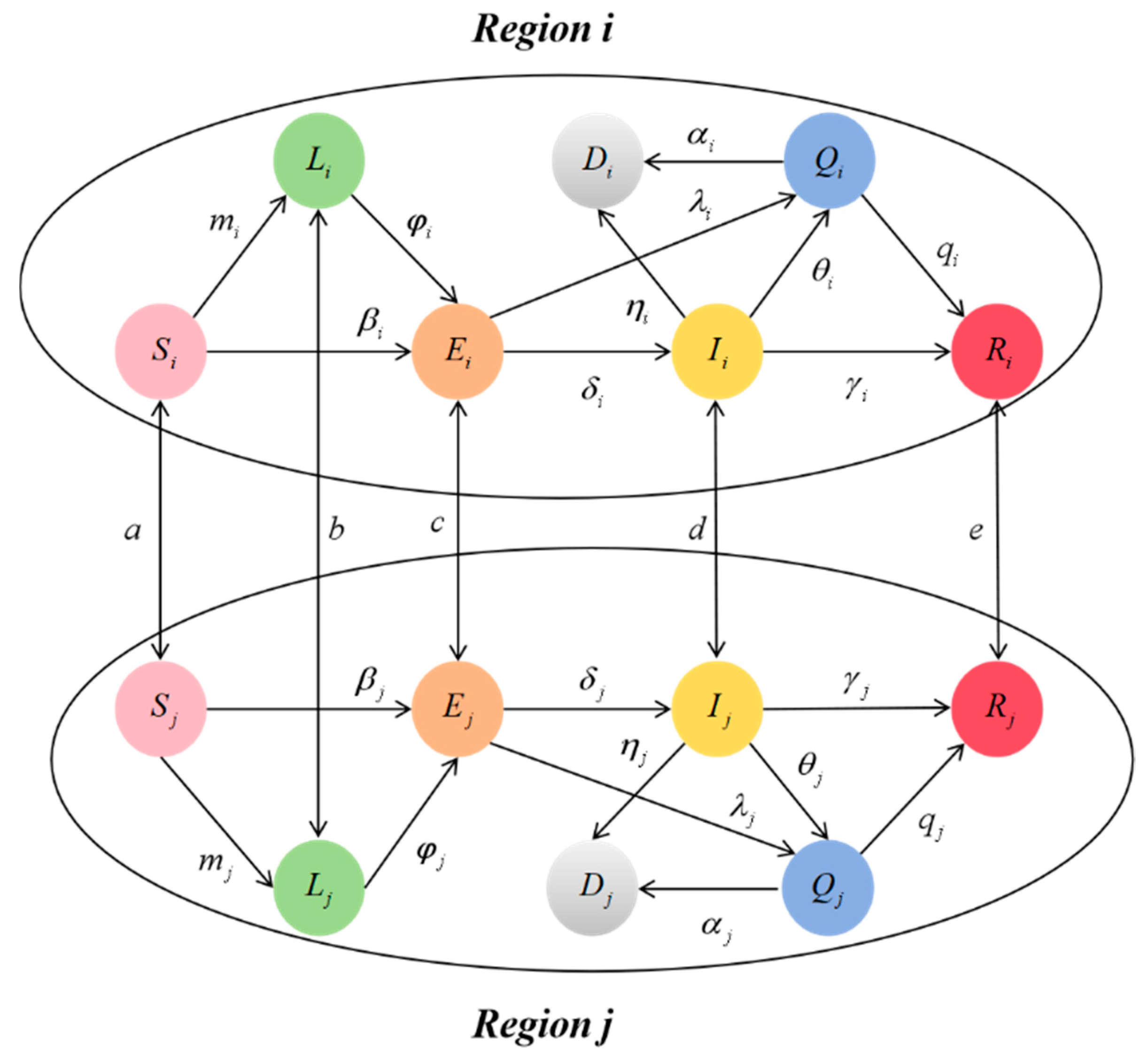
Based on the above assumption conditions, the state transition diagram of the model is shown in Figure 1.

3.2. Nonlinear Dynamic Model

Based on the state transition process in Figure 1, a new SLEIQDR transmission dynamic model is obtained as follows:

$$\left\{\begin{array}{l}{\displaystyle \frac{d{S}_i}{dt}}={\rho }_i{\mathrm{\Lambda }}_i-({\mu }_i+m_i)S_i-{\beta }_i{S}_i(E_i+I_i)+{\displaystyle \sum _{j=1}^n{a}_{ij}{S}_j-{\displaystyle \sum _{j=1}^n{a}_{ji}{S}_i}}\\ {\displaystyle \frac{d{L}_i}{dt}}=(1-{\rho }_i){\mathrm{\Lambda }}_i-{\mu }_i{L}_i+m_i{S}_i-{\phi }_i{L}_i(E_i+I_i)+{\displaystyle \sum _{j=1}^n{b}_{ij}{L}_j-{\displaystyle \sum _{j=1}^n{b}_{ji}{L}_i}}\\ {\displaystyle \frac{d{E}_i}{dt}}=({\beta }_i{S}_i+{\phi }_i{L}_i)(E_i+I_i)-({\mu }_i+{\lambda }_i+{\delta }_i)E_i+{\displaystyle \sum _{j=1}^n{c}_{ij}{E}_j-{\displaystyle \sum _{j=1}^n{c}_{ji}{E}_i}}\\ {\displaystyle \frac{d{I}_i}{dt}}={\delta }_i{E}_i-({\eta }_i+{\theta }_i+{\gamma }_i+{\mu }_i)I_i+{\displaystyle \sum _{j=1}^n{d}_{ij}{I}_j-{\displaystyle \sum _{j=1}^n{d}_{ji}{I}_i}}\\ {\displaystyle \frac{d{Q}_i}{dt}}={\theta }_i{I}_i+{\lambda }_i{E}_i-({\alpha }_i+q_i+{\mu }_i)Q_i\\ {\displaystyle \frac{d{D}_i}{dt}}={\alpha }_i{Q}_i+{\eta }_i{I}_i\\ {\displaystyle \frac{d{R}_i}{dt}}={\gamma }_i{I}_i+q_i{Q}_i-{\mu }_i{R}_i+{\displaystyle \sum _{j=1}^n{e}_{ij}{R}_j-{\displaystyle \sum _{j=1}^n{e}_{ji}{R}_i}}\end{array}\right.$$

(1)

where I ≠ j. If i = j, the migration rate is zero, and the model is transformed into a single region SLEIQDR model. The parameters in model (1) are defined in

Table 1. The definition of parameters in the model (1).

Symbol	Symbol Definition	Reference
ρi	The proportion of inputs to susceptible in the i-th region.	[1]
Λi	The constant input quantity in the i-th region.	[1]
μi	The natural mortality rate in the i-th region.	[40]
mi	The conversion rate of susceptible to low-risk in the i-th region.	Assumed
βi	The probability of susceptible being infected in the i-th region.	[46]
φi	The probability of low-risk individuals being infected in the i-th region.	Assumed
δi	The outbreak rate of exposure in the i-th region.	[46]
λi	The probability of the exposed being isolated in the i-th region.	[35]
ηi	The mortality rate of infected individuals in the i-th region due to illness.	[46]
θi	The probability of isolation for the infected in the i-th region.	[37]
γi	The recovery rate of infected in the i-th region.	[35]
αi	The mortality rate of those quarantined in the i-th region due to illness.	[46]
qi	The recovery rate of the quarantined in the i-th region.	[37]
aij,bij,cij,dij,eij	Migration rate of susceptible, low-risk, exposed, and infected individuals from region j to region i.	[33,40]

.

Due to the individuals who are quarantined, deceased, and recovered, they do not participate in the transmission of the disease within this model; therefore, the dynamical equations in Equation (1) are updated by

$$\left\{\begin{array}{l}{\displaystyle \frac{d{S}_i}{dt}}={\rho }_i{\mathrm{\Lambda }}_i-({\mu }_i+m_i)S_i-{\beta }_i{S}_i(E_i+I_i)+{\displaystyle \sum _{j=1}^n{a}_{ij}{S}_j-{\displaystyle \sum _{j=1}^n{a}_{ji}{S}_i}}\\ {\displaystyle \frac{d{L}_i}{dt}}=(1-{\rho }_i){\mathrm{\Lambda }}_i-{\mu }_i{L}_i+m_i{S}_i-{\phi }_i{L}_i(E_i+I_i)+{\displaystyle \sum _{j=1}^n{b}_{ij}{L}_j-{\displaystyle \sum _{j=1}^n{b}_{ji}{L}_i}}\\ {\displaystyle \frac{d{E}_i}{dt}}=({\beta }_i{S}_i+{\phi }_i{L}_i)(E_i+I_i)-({\mu }_i+{\lambda }_i+{\delta }_i)E_i+{\displaystyle \sum _{j=1}^n{c}_{ij}{E}_j-{\displaystyle \sum _{j=1}^n{c}_{ji}{E}_i}}\\ {\displaystyle \frac{d{I}_i}{dt}}={\delta }_i{E}_i-({\eta }_i+{\theta }_i+{\gamma }_i+{\mu }_i)I_i+{\displaystyle \sum _{j=1}^n{d}_{ij}{I}_j-{\displaystyle \sum _{j=1}^n{d}_{ji}{I}_i}}\end{array}\right.$$

(2)

Theorem 1.

The invariant set of system (1) is as follows:

$$\begin{array}{l}\mathrm{\Gamma }=\{(S_1,L_1,E_1,I_1,Q_1,D_1,R_1,...,S_n,L_n,E_n,I_n,Q_n,D_n,R_n)\in R_{+}^{7n}|N(t)\le {\displaystyle \frac{\widehat{\mathrm{\Lambda }}}{{\mu }^{*}}},\\ 0\le S_i\le S^0,0\le L_i\le L^0,i=1,2,\dots n\}\end{array}$$

(3)

where $\widehat{\mathrm{\Lambda }}={\displaystyle \sum _{i=1}^n{\mathrm{\Lambda }}_i,{\mu }^{*}=\min \left\{{\mu }_1\right.}\left.,{\mu }_2,\cdots ,{\mu }_n\right\}$, $S_i^0$ is the number of susceptible individuals when the system reaches the disease-free equilibrium point. And $L_i^0$ is the number of low-risk individuals when the system reaches the disease-free equilibrium point. And we have $N_i(t)=S_i(t)+L_i(t)+E_i(t)+I_i(t)+Q_i(t)+R_i(t),N(t)={\displaystyle \sum _{i=1}^n{N}_i(t)}$. N(t) is the total number of people alive.

Proof of Theorem 1.

The matrices A and B are defined as follows:

$$A_{ij}=\left\{\begin{array}{ll}{\mu }_i+m_i+{\displaystyle \sum _{k=1}^n{a}_{ki}}\hfill & if i=j\hfill \\ -a_{ij}\hfill & if i\ne j\hfill \end{array}\right.$$

(4)

$$B_{ij}=\left\{\begin{array}{ll}{\mu }_i+{\displaystyle \sum _{k=1}^n{b}_{ki}}\hfill & if i=j\hfill \\ -b_{ij}\hfill & if i\ne j\hfill \end{array}\right.$$

(5)

$$\begin{array}{l}{\displaystyle \frac{dN(t)}{dt}}={\displaystyle \sum _{i=1}^n\frac{d}{dt}(S_i(t)+L_i(t)+E_i(t)+I_i(t)+Q_i(t)+R_i(t))}\\ ={\displaystyle \sum _{i=1}^n{\mathrm{\Lambda }}_i-{\mu }_i(S_i(t)+L_i(t)+E_i(t)+I_i(t)+Q_i(t)+R_i(t))}+\\ {\displaystyle \sum _{i=1}^n{\displaystyle \sum _{j=1}^n[}}(a_{ij}{S}_j-a_{ji}{S}_i)+(b_{ij}{L}_j-b_{ji}{L}_i)+(c_{ij}{E}_j-c_{ji}{E}_i)+(d_{ij}{I}_j-d_{ji}{I}_i)+(e_{ij}{R}_j-e_{ji}{R}_i)]\\ =\widehat{\mathrm{\Lambda }}-{\displaystyle \sum _{i=1}^n{\mu }_i{N}_i(t)}+\xi \\ \le \widehat{\mathrm{\Lambda }}-{\mu }^{*}N(t)\end{array}$$

(6)

The migration item $\xi$ = 0. Solving the differential inequalities (6), we have $N(t)\le {\displaystyle \frac{\widehat{\mathrm{\Lambda }}}{{\mu }^{*}}}$ and

$$\left\{\begin{array}{l}{\displaystyle \frac{dS}{dt}}\le {\rho }_i{\mathrm{\Lambda }}_i-({\mu }_i+m_i)S_i+{\displaystyle \sum _{j=1}^n{a}_{ij}{S}_j-{\displaystyle \sum _{j=1}^n{a}_{ji}{S}_i={(A{S}^0-AS)}_i}}\\ {\displaystyle \frac{dL}{dt}}\le (1-{\rho }_i){\mathrm{\Lambda }}_i-\mu L_i+m_i{S}_i+{\displaystyle \sum _{j=1}^n{b}_{ij}{L}_j-{\displaystyle \sum _{j=1}^n{b}_{ji}{L}_i}={(B{L}^0-BL)}_i}\end{array}\right.$$

(7)

if i ≠ j, S_i = S_i⁰, S_j ≤ S_j⁰, ${\displaystyle \frac{dS}{dt}}\le 0$, L_i = L_i⁰, L_j ≤ L_j⁰, ${\displaystyle \frac{dL}{dt}}\le 0$. So we have S_i ≤ S_i⁰, L_i ≤ L_i⁰. The proof is now complete. □

Theorem 2.

System (2) has a unique disease-free equilibrium.

Proof of Theorem 2.

Let the right-hand side of the Equation (2) be zero, and E_i = 0 and I_i = 0 are substituted into the Equation (2), the result is obtained as follows:

$$\left\{\begin{array}{l}{\rho }_i{\mathrm{\Lambda }}_i-({\mu }_i+m_i)S_i+{\displaystyle \sum _{j=1}^n{a}_{ij}{S}_j-{\displaystyle \sum _{j=1}^n{a}_{ji}{S}_i=0}}\\ (1-{\rho }_i){\mathrm{\Lambda }}_i-{\mu }_i{L}_i+m_i{S}_i+{\displaystyle \sum _{j=1}^n{b}_{ij}{L}_j-{\displaystyle \sum _{j=1}^n{b}_{ji}{L}_i}}=0\end{array}\right.$$

(8)

furthermore, its matrix forms are described by

$$\left(\begin{array}{cc}A& 0\\ C& B\end{array}\right)\left(\begin{array}{c}S\\ L\end{array}\right)=\left(\begin{array}{c}{M}_s\\ M_l\end{array}\right)$$

(9)

A and B maintain the definitions of Equations (4) and (5). C = −diag (m₁, m₂, m₃, …, m_n)^T. And M_s = (ρ₁Λ₁, ρ₂Λ₂, ρ₃Λ₃, …, ρ_nΛ_n)^T, M_l = ((1 − ρ₁)Λ₁, (1 − ρ₂)Λ₂, (1 − ρ₃)Λ₃, …, (1 − ρ_n)Λ_n)^T, S = (S₁, S₂, S₃, …, S_n)^T, L = (L₁, L₂, L₃, …, L_n)^T.

Because the sum of each column in matrices A and B is greater than zero, and the non-diagonal elements are non-positive, there exists a unique solution for the disease-free equilibrium, which can be expressed as S₀ = A⁻¹M_s, L₀ = B⁻¹(M_l − CA⁻¹M_s). □

According to the system (2) and the matrix-based next-generation approach, the model’s basic reproduction number R₀ is calculated, where F_E = (β_iS_i + φ_iL_i)(E_i + I_i), F_I = 0, V_E =(μ_i + λ_i + δ_i)E_i − ${\displaystyle \sum _{j=1}^n{c}_{ij}{E}_j+}{\displaystyle \sum _{j=1}^n{c}_{ji}{E}_i}$, V_I = (η_i + θ_i + γ_i)I_i – δ_iE_i – ${\displaystyle \sum _{j=1}^n{d}_{ij}{I}_j+}{\displaystyle \sum _{j=1}^n{d}_{ji}{I}_i}$, therefore

$$F=\left(\begin{array}{cc}{F}_1& F_1\\ 0& 0\end{array}\right)$$

(10)

$$V=\left(\begin{array}{cc}{v}_1& 0\\ v_2& v_3\end{array}\right)$$

(11)

$$F_1=diag({\beta }_1{S}_1^0+{\phi }_1{L}_1^0,\dots ,{\beta }_n{S}_n^0+{\phi }_n{L}_n^0)$$

(12)

$$v_1=diag({\mu }_1+{\delta }_1+{\lambda }_1,\dots ,{\mu }_n+{\delta }_n+{\lambda }_n)+diag(s_c)-ℂ$$

(13)

where s_c is the sum of the column vectors of the matrix $ℂ$, and $s_{C,i}={\displaystyle \sum _{j=1}^n{c}_{ji}}$. The matrix $ℂ$ is the migration matrix corresponding to exposed. Similarly, $v_2$ and $v_3$ are defined as follows:

$$v_2=-diag({\delta }_1,\dots {\delta }_n)$$

(14)

$$v_3=diag({\eta }_1+{\theta }_1+{\gamma }_1+{\mu }_1,\dots ,{\eta }_n+{\theta }_n+{\gamma }_n+{\mu }_n)+diag(s_{D^{\prime }})-D^{\prime }$$

(15)

where $s_{D^{\prime }}$ is the sum of the column vectors of matrix $D^{\prime }$, that is $s_{D^{\prime },i}={\displaystyle \sum _{j=1}^n{d}_{ji}}$. The matrix $D^{\prime }$ is the migration matrix corresponding to the infected.

F and V are 2n × 2n matrices, and v₁ and v₃ are both reversible matrices.

$$F{V}^{-1}=\left(\begin{array}{cc}{F}_1& F_1\\ 0& 0\end{array}\right)\left(\begin{array}{cc}{v}_1^{-1}& 0\\ -v_3^{-1}{v}_2{v}_1^{-1}& v_3^{-1}\end{array}\right)=\left(\begin{array}{cc}{F}_1{v}_1^{-1}-F_1{v}_3^{-1}{v}_2{v}_1^{-1}& F_1{v}_3^{-1}\\ 0& 0\end{array}\right)$$

(16)

As a result, the R₀ is obtained as follows:

$$R_0=\rho (F{V}^{-1})=\rho (F_1{v}_1^{-1}-F_1{v}_3^{-1}{v}_2{v}_1^{-1})$$

(17)

For a single region, the R₀ is calculated by

$$R_0^{(i)}=\rho (F_i{V}_i^{-1})={\displaystyle \frac{({\beta }_i{S}_i^0+{\phi }_i{L}_i^0){\delta }_i}{({\delta }_i+{\mu }_i+{\lambda }_i)({\gamma }_i+{\mu }_i+{\eta }_i+{\theta }_i)}}+{\displaystyle \frac{({\beta }_i{S}_i^0+{\phi }_i{L}_i^0)}{({\delta }_i+{\mu }_i+{\lambda }_i)}}$$

(18)

Theorem 3.

If ${\delta }_i=\delta ,{\delta }_i+{\mu }_i+{\lambda }_i=a_i=a,{\beta }_i{S}_i^0+{\phi }_i{L}_i^0={\sigma }_i,{\gamma }_i+{\mu }_i+{\eta }_i+{\theta }_i=b_i=b$ , ${\sigma }_1\le {\sigma }_2\le \cdots \le {\sigma }_n$ and then $R_0^{(i)}={\displaystyle \frac{{\sigma }_i{\delta }_i}{a_i{b}_i}}+{\displaystyle \frac{{\sigma }_i}{a_i}}$, $\underset{1\le i\le n}{min}{R}_0^{(i)}\le R_0\le \underset{1\le i\le n}{max}{R}_0^{(i)}$.

Proof of Theorem 3.

Let v₁⁻¹ = P, v₃⁻¹ = L, W = F₁P − F₁LV₂P, ${\sigma }_1\le {\sigma }_2\le \cdots \le {\sigma }_n$ , the sum of the i-th column of matrix v₁ is a_i, and a_{i =} a. That is,

$${\displaystyle \sum _{i=1}^n{(v_1)}_{ij}}=a,\hspace{1em}\forall j\in \{1,\dots ,n\}.$$

(19)

This implies that the unit row vector e^T = [1, 1, …, 1] is a left eigenvector of ν₁ with eigenvalue a:

$$e^T{v}_1=a{e}^T$$

(20)

Let ν₁⁻¹ denote the inverse of ν₁. Then, scaling ν₁⁻¹ by a yields a matrix B = a ν₁⁻¹ whose columns sum to unity:

$${\displaystyle \sum _{i=1}^n{B}_{ij}}=1,\hspace{1em}\forall j\in \{1,\dots ,n\}$$

(21)

From (20), we have

$$e^T{v}_1{v}_1^{-1}=a{e}^T{v}_1^{-1}\Rightarrow e^{T}I=a{e}^T{v}_1^{-1}\Rightarrow e^T=a{e}^T{v}_1^{-1}$$

(22)

where I is the identity matrix. Rearranging (22), we obtain the following:

$$e^T{v}_1^{-1}={\displaystyle \frac{1}{a}}{e}^T.$$

(23)

The column sums of B are

$${\displaystyle \sum _{i=1}^n{B}_{ij}}={\displaystyle \sum _{i=1}^{n}a}{({\nu }_1^{-1})}_{ij}=a\left({\displaystyle \sum _{i=1}^n{({\nu }_1^{-1})}_{ij}}\right)=a\cdot {\displaystyle \frac{1}{a}}=1$$

(24)

where ${\displaystyle \sum _{i=1}^n{a}_i{P}_{ij}}=1$, ${\displaystyle \sum _{i=1}^n{P}_{ij}}={\displaystyle \frac{1}{a}}$. Similarly, ${\displaystyle \sum _{i=1}^n{l}_{ij}}={\displaystyle \frac{1}{b}}$. Therefore, the sum of the j-th column of matrix W is calculated as follows:

$$\begin{array}{l}{\displaystyle \sum _{i=1}^n{w}_{ij}=}{\displaystyle \sum _{i=1}^n({\beta }_i{S}_i^0+{\phi }_i{L}_i^0)}{v}_{1_{(i,j)}}^{-1}+{\displaystyle \sum _{i=1}^n{\displaystyle \sum _{k=1}^n({\beta }_i{S}_i^0+{\phi }_i{L}_i^0)}}{\delta }_k{v}_{3_{(i,k)}}^{-1}{v}_{1_{(i,k)}}^{-1}\\ ={\displaystyle \sum _{i=1}^n{\sigma }_i{P}_{ij}}+{\displaystyle \sum _{i=1}^n{\sigma }_i{\displaystyle \sum _{k=1}^n{\delta }_k{l}_{ik}{P}_{kj}}}\le {\sigma }_n{\displaystyle \sum _{i=1}^n{P}_{ij}}+{\sigma }_n\delta {\displaystyle \sum _{i=1}^n{\displaystyle \sum _{k=1}^n{l}_{ik}{P}_{kj}}}\\ ={\displaystyle \frac{{\sigma }_n}{a}}+{\displaystyle \frac{{\sigma }_n\delta }{ab}}=R_0^{(n)}\end{array}$$

(25)

Similarly, ${\displaystyle \sum _{i=1}^n{w}_{ij}\ge \frac{{\sigma }_1}{a}+\frac{{\sigma }_1\delta }{ab}=R_0^{(1)}}$. So $\underset{1\le i\le n}{min}{R}_0^{(i)}\le R_0\le \underset{1\le i\le n}{max}{R}_0^{(i)}$. □

In some cases, due to strict control measures, the exposed and infected may not migrate between different regions. Therefore. c_ij = c_ji = d_ij = d_ji = 0, i, j = 1, …, n, and v₁ and v₃ are updated as follows

$$v_1=diag({\mu }_1+{\delta }_1+{\lambda }_1,\dots ,{\mu }_n+{\delta }_n+{\lambda }_n)$$

(26)

$$v_3=diag({\eta }_1+{\theta }_1+{\gamma }_1+{\mu }_1,\dots ,{\eta }_n+{\theta }_n+{\gamma }_n+{\mu }_n)$$

(27)

The R₀ is obtained by

$$R_0=\rho (F{V}^{-1})=\rho (F_1{v}_1^{-1}-F_1{v}_3^{-1}{v}_2{v}_1^{-1})=\underset{1\le i\le n}{max}{R}_0^{(i)}$$

(28)

4. Dynamics Behavior Analysis of the Model

4.1. Global Stability Analysis of Disease-Free Equilibrium

Theorem 4.

If R₀ < 1, the system (2) is globally asymptotically stable at the disease-free equilibrium.

Proof of Theorem 4.

A Lyapunov function is presented as

$$L_i={\displaystyle \sum _{i=1}^n{h}_i{E}_i}+{\displaystyle \sum _{i=1}^n{l}_i{I}_i}$$

(29)

The weights h_i and l_i in the Lyapunov function $L_i={\displaystyle \sum _{i=1}^n{h}_i{E}_i}+{\displaystyle \sum _{i=1}^n{l}_i{I}_i}$ are constructed from the left eigenvector of the matrix V⁻¹F, corresponding to its spectral radius R₀. We set h_i = f_i and l_i = r_i. This ensures ${\displaystyle \frac{dL}{dt}}\le 0$ when R₀ < 1.

The derivative of L_i in the system (2) is obtained as follows:

$$\begin{array}{l}{\displaystyle \frac{d{L}_i}{dt}}=h_i{\displaystyle \sum _{i=1}^n\frac{d{E}_i}{dt}}+l_i{\displaystyle \sum _{i=1}^n\frac{d{I}_i}{dt}}\\ =h_i{\displaystyle \sum _{i=1}^n\left[({\beta }_i{S}_i+{\phi }_i{L}_i)(E_i+I_i)-({\mu }_i+{\lambda }_i+{\delta }_i)E_i+{\displaystyle \sum _{j=1}^n{c}_{ij}{E}_j-{\displaystyle \sum _{j=1}^n{c}_{ji}{E}_i}}\right]}\\ +l_i{\displaystyle \sum _{i=1}^n\left[{\delta }_i{E}_i-({\eta }_i+{\theta }_i+{\gamma }_i+{\mu }_i)I_i+{\displaystyle \sum _{j=1}^n{d}_{ij}{I}_j-{\displaystyle \sum _{j=1}^n{d}_{ji}{I}_i}}\right]}\\ \le h_i{\displaystyle \sum _{i=1}^n\left[({\beta }_i{S}_i^0+{\phi }_i{L}_i^0)(E_i+I_i)-({\mu }_i+{\lambda }_i+{\delta }_i)E_i+{\displaystyle \sum _{j=1}^n{c}_{ij}{E}_j-{\displaystyle \sum _{j=1}^n{c}_{ji}{E}_i}}\right]}\\ +l_i{\displaystyle \sum _{i=1}^n\left[{\delta }_i{E}_i-({\eta }_i+{\theta }_i+{\gamma }_i+{\mu }_i)I_i+{\displaystyle \sum _{j=1}^n{d}_{ij}{I}_j-{\displaystyle \sum _{j=1}^n{d}_{ji}{I}_i}}\right]}\\ =\left(k_1,k_2,\cdots k_n,v_1,v_2,\cdots v_n\right)\left[(F-V){(E_1,E_2,\cdots E_n,I_1,I_2,\cdots I_n)}^T\right]\\ =\left(k_1,k_2,\cdots k_n,v_1,v_2,\cdots v_n\right)\left[(F-V)M\right]\\ =\left(f_1,f_2,\cdots f_n,r_1,r_2,\cdots r_n\right)V^{-1}\left[(F-V)M\right]\\ =\left(f_1,f_2,\cdots f_n,r_1,r_2,\cdots r_n\right)(V^{-1}F-E)M\\ =\left(f_1,f_2,\cdots f_n,r_1,r_2,\cdots r_n\right)(\rho \left(F{V}^{-1}\right)-1)M\\ \le 0\end{array}$$

(30)

where the vector $\left(f_1,f_2,\cdots f_n,r_1,r_2,\cdots r_n\right)$ is the left eigenvector of V⁻¹F. If ${\displaystyle \frac{d{L}_i}{dt}}=0$, S_i = S_i⁰, E_i = 0, I_i = 0. According to the result of Theorem 1 and the Lasalle invariant set principle, if R₀ < 1, the system (2) is globally asymptotically stable at the disease-free equilibrium. □

4.2. Global Stability Analysis of Endemic Disease Equilibrium

Theorem 5.

The endemic disease equilibrium exists and is unique.

Proof of Theorem 5.

First, we prove the existence of the Endemic Equilibrium. We prove existence using the mapping method. Define the ${\mathrm{\Psi }}_i=E_i+I_i>0$ , and construct a mapping G:${ℝ}_{+}^n\to {ℝ}_{+}^n$, where $G(\mathrm{\Psi })=(G_1(\mathrm{\Psi }),\dots ,G_n(\mathrm{\Psi }))$ is determined by as follows:

$$\left\{\begin{array}{l}{S}_i\left({\mu }_i+m_i+{\beta }_i{\mathrm{\Psi }}_i\right)={\rho }_i{\mathrm{\Lambda }}_i+{\displaystyle \sum _{j=1}^n{a}_{ij}}{S}_j-{\displaystyle \sum _{j=1}^n{a}_{ji}}{S}_i,\hfill \\ L_i\left({\mu }_i+{\varphi }_i{\mathrm{\Psi }}_i\right)=(1-{\rho }_i){\mathrm{\Lambda }}_i+m_i{S}_i+{\displaystyle \sum _{j=1}^n{b}_{ij}}{L}_j-{\displaystyle \sum _{j=1}^n{b}_{ji}}{L}_i\hfill \end{array}\right.$$

(31)

Since the coefficient matrix is an M-matrix and the right-hand side is positive, there exists a unique positive solution $S_i\left(\mathrm{\Psi }\right)>0$, $L_i\left(\mathrm{\Psi }\right)>0$, and $S_i\left(\mathrm{\Psi }\right)$, $L_i\left(\mathrm{\Psi }\right)$ are continuously decreasing with respect to ${\mathrm{\Psi }}_i$. Calculate the new infection input as follows:

$$A_i(\mathrm{\Psi })=({\beta }_i{S}_i(\mathrm{\Psi })+{\varphi }_i{L}_i(\mathrm{\Psi })){\mathrm{\Psi }}_i$$

(32)

Solve the $E_i(\mathrm{\Psi })$ and $I_i(\mathrm{\Psi })$:

$$\left\{\begin{array}{l}({\delta }_i+{\mu }_i+{\lambda }_i)E_i=A_i(\mathrm{\Psi })+{\displaystyle \sum _{j=1}^n{c}_{ij}}{E}_j-{\displaystyle \sum _{j=1}^n{c}_{ji}}{E}_i\hfill \\ ({\theta }_i+{\lambda }_i+{\mu }_i+{\eta }_i)I_i={\delta }_i{E}_i+{\displaystyle \sum _{j=1}^n{d}_{ij}}{I}_j-{\displaystyle \sum _{j=1}^n{d}_{ji}}{E}_i\hfill \end{array}\right.$$

(33)

Since the coefficient matrices are M-matrices, there exists a unique solution $E_i(\mathrm{\Psi })\ge 0$, $I_i\left(\mathrm{\Psi }\right)\ge 0$. We define $G_i\left(\mathrm{\Psi }\right)=E_i\left(\mathrm{\Psi }\right)+I_i\left(\mathrm{\Psi }\right)$. $G(0)=0$, G is continuous and monotonically increasing. $\Vert \mathrm{\Psi }\Vert \to \infty$$G(\mathrm{\Psi })\to 0$. The spectral radius of the Jacobian matrix of G at $\mathrm{\Psi }=0$ equals R₀. Since R₀ > 1, there exists $\mathrm{u}>0$ such that G(u) > u. Consider the $X=\{\mathrm{\Psi }\ge 0\mid G(\mathrm{\Psi })\ge \mathrm{\Psi }\}$, which is non-empty and bounded. Let ${\mathrm{\Psi }}^{*}=\sup X$, and by the continuity of G, we have $G({\mathrm{\Psi }}^{*})={\mathrm{\Psi }}^{*}$ with ${\mathrm{\Psi }}^{*}>0$. From ${\mathrm{\Psi }}^{*}$, we can uniquely determine $S_i^{*}=S_i\left({\mathrm{\Psi }}^{*}\right)>0$, $L_i^{*}=L_i\left({\mathrm{\Psi }}^{*}\right)>0,$, $,E_i^{*}=E_i\left({\mathrm{\Psi }}^{*}\right)>0$, $,I_i^{*}=I_i\left({\mathrm{\Psi }}^{*}\right)>0$. Solving the equilibrium equations for $Q_i^{*}$ and $R_i^{*}$ yields all state variables strictly positive, forming an endemic equilibrium. Then we prove the Uniqueness of the Endemic Equilibrium. First, we show that the mapping G satisfies the sublinearity condition:

$$G(c\mathrm{\Psi })\ge cG(\mathrm{\Psi }),\hspace{1em}\forall c\in [0,1],\forall \mathrm{\Psi }\ge 0$$

(34)

This property holds because $S_i\left({\mathrm{\Psi }}^{*}\right)$ and $L_i\left({\mathrm{\Psi }}^{*}\right)$ are convex functions with respect to ${\mathrm{\Psi }}_i$, The new infection input $A_i(\mathrm{\Psi })$ is concave with respect to ${\mathrm{\Psi }}_i$, and the inverse of an M-matrix preserves the sublinearity structure. Suppose ${\mathrm{\Psi }}^{*}$ and ${\mathrm{\Psi }}^{**}$ are both positive fixed points of G. Define:

$$c={\min }_{1\le i\le n}{\displaystyle \frac{{\mathrm{\Psi }}_i^{**}}{{\mathrm{\Psi }}_i^{*}}}\in (0,1]$$

(35)

Then $c{\mathrm{\Psi }}^{*}\le {\mathrm{\Psi }}^{**}$ and there exists k such that $c{\mathrm{\Psi }}_k^{*}={\mathrm{\Psi }}_k^{**}$. By the sublinearity condition and monotonicity of G:

$${\mathrm{\Psi }}^{**}=G({\mathrm{\Psi }}^{**})\ge G(c{\mathrm{\Psi }}^{*})\ge cG({\mathrm{\Psi }}^{*})=c{\mathrm{\Psi }}^{*}$$

(36)

If c < 1, consider the iterative sequence ${\mathrm{\Psi }}^{(0)}=c{\mathrm{\Psi }}^{*}$, ${\mathrm{\Psi }}^{(k+1)}=G({\mathrm{\Psi }}^{(k)})$. By the sublinearity condition, ${\mathrm{\Psi }}^{(0)}\le {\mathrm{\Psi }}^{(1)}$, and by monotonicity, $\left\{{\mathrm{\Psi }}^{(k)}\right\}$ is monotonically increasing and converges to some limit $\widehat{\mathrm{\Psi }}\ge c{\mathrm{\Psi }}^{*}$ satisfying $G(\widehat{\mathrm{\Psi }})=\widehat{\mathrm{\Psi }}$. Since $\widehat{\mathrm{\Psi }}\le {\mathrm{\Psi }}^{**}$ and G is strictly sublinear in the positive region, the iterative sequence converges strictly increasing to ${\mathrm{\Psi }}^{**}$. However, if c < 1, then ${\mathrm{\Psi }}^{(1)}>{\mathrm{\Psi }}^{(0)}$, which contradicts $\widehat{\mathrm{\Psi }}$ being the limit unless c = 1. Therefore, c = 1, which implies ${\mathrm{\Psi }}^{**}={\mathrm{\Psi }}^{*}$. Since $\mathrm{\Psi }$ uniquely determines all state variables, the endemic equilibrium is unique. □

Theorem 6.

Assuming that the transfer matrices AT = (a_ij), BT = (b_ij), CT = (c_ij), DT = (d_ij) are all irreducible, if R₀ > 1, the endemic equilibrium in the system (2) holds the following condition on the feasible region Γ, where

$$\left\{\begin{array}{l}1,\exists {\eta }_1,{\eta }_2,{\eta }_3,{\eta }_4, let{\eta }_1{a}_{ij}{S}_j^{*}={\eta }_2{b}_{ij}{L}_j^{*}={\eta }_3{c}_{ij}{E}_j^{*}={\eta }_4{d}_{ij}{I}_j^{*}\\ 2,({\beta }_i{S}_i^{*}+{\phi }_i{L}_i^{*})I_i(1-{\displaystyle \frac{I_i^{*}{E}_i}{I_i{E}_i^{*}}})+({\beta }_i{S}_i+{\phi }_i{L}_i)I_i^{*}(1-{\displaystyle \frac{I_i{E}_i^{*}}{I_i^{*}{E}_i}})+{\delta }_i{E}_i(1-{\displaystyle \frac{I_i^{*}}{I_i}})+{\delta }_i{E}_i^{*}(1-{\displaystyle \frac{I_i}{I_i^{*}}})\\ +m_i{S}_i(1-{\displaystyle \frac{L_i^{*}}{L_i}})+m_i{S}_i^{*}(1-{\displaystyle \frac{L_i}{L_i^{*}}})<0\end{array}\right.$$

(37)

The endemic equilibrium E^* of the system (2) is unique and globally asymptotically stable in the feasible region Γ.

Proof of Theorem 6.

We construct the Lyapunov function as follows.

$$V_i(S_i,L_i,E_i,I_i)=S_i-S_i^{*}-S_i^{*}\ln {\displaystyle \frac{S_i}{S_i^{*}}}+L_i-L_i^{*}-L_i^{*}\ln {\displaystyle \frac{L_i}{L_i^{*}}}+E_i-E_i^{*}-E_i^{*}\ln {\displaystyle \frac{E_i}{E_i^{*}}}+I_i-I_i^{*}-I_i^{*}\ln {\displaystyle \frac{I_i}{I_i^{*}}}$$

(38)

The derivative of the function V_i (S_i, L_i, E_i, I_i) in Equation (2) is

$$\begin{array}{l}{\displaystyle \frac{d{V}_i}{dt}}=(1-{\displaystyle \frac{S_i^{*}}{S_i}}){\displaystyle \frac{d{S}_i}{dt}}+(1-{\displaystyle \frac{L_i^{*}}{L_i}}){\displaystyle \frac{d{L}_i}{dt}}+(1-{\displaystyle \frac{E_i^{*}}{E_i}}){\displaystyle \frac{d{E}_i}{dt}}+(1-{\displaystyle \frac{I_i^{*}}{I_i}}){\displaystyle \frac{d{I}_i}{dt}}\\ =(1-{\displaystyle \frac{S_i^{*}}{S_i}})({\rho }_i{\mathrm{\Lambda }}_i-({\mu }_i+m_i)S_i-{\beta }_i{S}_i(E_i+I_i)+{\displaystyle \sum _{j=1}^n{a}_{ij}{S}_j-{\displaystyle \sum _{j=1}^n{a}_{ji}{S}_i}})\\ +(1-{\displaystyle \frac{L_i^{*}}{L_i}})((1-{\rho }_i){\mathrm{\Lambda }}_i-\mu L_i+m_i{S}_i-{\phi }_i{L}_i(E_i+I_i)+{\displaystyle \sum _{j=1}^n{b}_{ij}{L}_j-{\displaystyle \sum _{j=1}^n{b}_{ji}{L}_i}})\\ +(1-{\displaystyle \frac{E_i^{*}}{E_i}})(({\beta }_i{S}_i+{\phi }_i{L}_i)(E_i+I_i)-({\mu }_i+{\lambda }_i+{\delta }_i)E_i+{\displaystyle \sum _{j=1}^n{c}_{ij}{E}_j-{\displaystyle \sum _{j=1}^n{c}_{ji}{E}_i}})\\ +(1-{\displaystyle \frac{I_i^{*}}{I_i}}\left)\right({\delta }_i{E}_i-({\eta }_i+{\theta }_i+{\gamma }_i+{\mu }_i)I_i+{\displaystyle \sum _{j=1}^n{d}_{ij}{I}_j-{\displaystyle \sum _{j=1}^n{d}_{ji}{I}_i}})\end{array}$$

(39)

According to the system (2), it can be obtained by

$$\left\{\begin{array}{l}({\mu }_i+m_i)S_i^{*}={\rho }_i{\mathrm{\Lambda }}_i-{\beta }_i{S}_i^{*}(E_i^{*}+I_i^{*})+{\displaystyle \sum _{j=1}^n{a}_{ij}{S}_j^{*}-{\displaystyle \sum _{j=1}^n{a}_{ji}{S}_i^{*}}}\\ \mu L_i^{*}=(1-{\rho }_i){\mathrm{\Lambda }}_i+m_i{S}_i^{*}-{\phi }_i{L}_i^{*}(E_i^{*}+I_i^{*})+{\displaystyle \sum _{j=1}^n{b}_{ij}{L}_j^{*}-{\displaystyle \sum _{j=1}^n{b}_{ji}{L}_i^{*}}}\\ ({\mu }_i+{\lambda }_i+{\delta }_i)E_i^{*}=({\beta }_i{S}_i^{*}+{\phi }_i{L}_i^{*})(E_i^{*}+I_i^{*})+{\displaystyle \sum _{j=1}^n{c}_{ij}{E}_j^{*}-{\displaystyle \sum _{j=1}^n{c}_{ji}{E}_i^{*}}}\\ ({\eta }_i+{\theta }_i+{\gamma }_i+{\mu }_i)I_i^{*}={\delta }_i{E}_i^{*}+{\displaystyle \sum _{j=1}^n{d}_{ij}{I}_j^{*}-{\displaystyle \sum _{j=1}^n{d}_{ji}{I}_i^{*}}}\end{array}\right.$$

(40)

Equation (40) is substituted into Equation (39), and the result is obtained as follows:

$$\begin{gathered} \begin{array}{l}{\rho }_i{\mathrm{\Lambda }}_i(1-{\displaystyle \frac{S_i^{*}}{S_i}}+1-{\displaystyle \frac{S_i}{S_i^{*}}})+{\beta }_i{S}_i(E_i^{*}+I_i^{*})+{\beta }_i{S}_i^{*}(E_i+I_i)+{\displaystyle \sum _{j=1}^n{a}_{ij}{S}_j-{\displaystyle \sum _{j=1}^n{a}_{ij}{S}_j\frac{S_i^{*}}{S_i}}}\\ +{\displaystyle \sum _{j=1}^n{a}_{ij}{S}_j^{*}-}{\displaystyle \sum _{j=1}^n{a}_{ij}{S}_j^{*}\frac{S_i}{S_i^{*}}}+(1-{\rho }_i){\mathrm{\Lambda }}_i(1-{\displaystyle \frac{L_i^{*}}{L_i}}+1-{\displaystyle \frac{L_i}{L_i^{*}}})+m_i(S_i+S_i^{*})-S_i{\displaystyle \frac{L_i^{*}}{L_i}}-S_i^{*}{\displaystyle \frac{L_i}{L_i^{*}}}+{\phi }_i{L}_i(E_i^{*}+I_i^{*})\\ +{\phi }_i{L}_i^{*}(E_i+I_i)+{\displaystyle \sum _{j=1}^n{b}_{ij}{L}_j-{\displaystyle \sum _{j=1}^n{b}_{ij}{L}_j\frac{L_i^{*}}{L_i}}}+{\displaystyle \sum _{j=1}^n{b}_{ij}{L}_j^{*}-}{\displaystyle \sum _{j=1}^n{b}_{ij}{L}_j^{*}\frac{L_i}{L_i^{*}}}-({\beta }_i{S}_i^{*}+{\phi }_i{L}_i^{*})(E_i^{*}+I_i^{*}){\displaystyle \frac{E_i}{E_i^{*}}}\\ -({\beta }_i{S}_i+{\phi }_i{L}_i)(E_i+I_i){\displaystyle \frac{E_i^{*}}{E_i}}+{\displaystyle \sum _{j=1}^n{c}_{ij}{E}_j-{\displaystyle \sum _{j=1}^n{c}_{ij}{E}_j\frac{E_i^{*}}{E_i}}}+{\displaystyle \sum _{j=1}^n{c}_{ij}{E}_j^{*}-}{\displaystyle \sum _{j=1}^n{c}_{ij}{E}_j^{*}\frac{E_i}{E_i^{*}}}+{\delta }_i(E_i^{*}+E_i-E_i^{*}{\displaystyle \frac{I_i}{I_i^{*}}}-E_i{\displaystyle \frac{I_i^{*}}{I_i}})\\ +{\displaystyle \sum _{j=1}^n{d}_{ij}{I}_j-{\displaystyle \sum _{j=1}^n{d}_{ij}{I}_j\frac{I_i^{*}}{I_i}}}+{\displaystyle \sum _{j=1}^n{d}_{ij}{I}_j^{*}-}{\displaystyle \sum _{j=1}^n{d}_{ij}{I}_j^{*}\frac{I_i}{I_i^{*}}}\\ \le {\beta }_i{S}_i(E_i^{*}+I_i^{*})+{\beta }_i{S}_i^{*}(E_i+I_i)+{\displaystyle \sum _{j=1}^n{a}_{ij}{S}_j-{\displaystyle \sum _{j=1}^n{a}_{ij}{S}_j\frac{S_i^{*}}{S_i}}}+{\displaystyle \sum _{j=1}^n{a}_{ij}{S}_j^{*}-}{\displaystyle \sum _{j=1}^n{a}_{ij}{S}_j^{*}\frac{S_i}{S_i^{*}}}\\ +m_i(S_i+S_i^{*})-S_i{\displaystyle \frac{L_i^{*}}{L_i}}-S_i^{*}{\displaystyle \frac{L_i}{L_i^{*}}}+{\phi }_i{L}_i(E_i^{*}+I_i^{*})+{\phi }_i{L}_i^{*}(E_i+I_i)+{\displaystyle \sum _{j=1}^n{b}_{ij}{L}_j-{\displaystyle \sum _{j=1}^n{b}_{ij}{L}_j\frac{L_i^{*}}{L_i}}}+{\displaystyle \sum _{j=1}^n{b}_{ij}{L}_j^{*}-}{\displaystyle \sum _{j=1}^n{b}_{ij}{L}_j^{*}\frac{L_i}{L_i^{*}}}\\ -({\beta }_i{S}_i^{*}+{\phi }_i{L}_i^{*})(E_i^{*}+I_i^{*}){\displaystyle \frac{E_i}{E_i^{*}}}-({\beta }_i{S}_i+{\phi }_i{L}_i)(E_i+I_i){\displaystyle \frac{E_i^{*}}{E_i}}+{\displaystyle \sum _{j=1}^n{c}_{ij}{E}_j-{\displaystyle \sum _{j=1}^n{c}_{ij}{E}_j\frac{E_i^{*}}{E_i}}}+{\displaystyle \sum _{j=1}^n{c}_{ij}{E}_j^{*}-}{\displaystyle \sum _{j=1}^n{c}_{ij}{E}_j^{*}\frac{E_i}{E_i^{*}}}\\ +{\delta }_i(E_i^{*}+E_i-E_i^{*}{\displaystyle \frac{I_i}{I_i^{*}}}-E_i{\displaystyle \frac{I_i^{*}}{I_i}})+{\displaystyle \sum _{j=1}^n{d}_{ij}{I}_j-{\displaystyle \sum _{j=1}^n{d}_{ij}{I}_j\frac{I_i^{*}}{I_i}}}+{\displaystyle \sum _{j=1}^n{d}_{ij}{I}_j^{*}-}{\displaystyle \sum _{j=1}^n{d}_{ij}{I}_j^{*}\frac{I_i}{I_i^{*}}}\end{array} \\ \begin{array}{l}={\beta }_i{S}_i(E_i^{*}+I_i^{*})+{\beta }_i{S}_i^{*}(E_i+I_i)+{\displaystyle \sum _{j=1}^n{a}_{ij}{S}_j^{*}(1-\frac{S_j{S}_i^{*}}{S_j^{*}{S}_i}+\ln \frac{S_j{S}_i^{*}}{S_j^{*}{S}_i})+}{\displaystyle \sum _{j=1}^n{a}_{ij}{S}_j^{*}(\frac{S_j}{S_j^{*}}-\frac{S_i}{S_i^{*}}-\ln \frac{S_j}{S_j^{*}}-\ln \frac{S_i^{*}}{S_i})}\\ +m_i(S_i+S_i^{*})-S_i{\displaystyle \frac{L_i^{*}}{L_i}}-S_i^{*}{\displaystyle \frac{L_i}{L_i^{*}}}+{\phi }_i{L}_i(E_i^{*}+I_i^{*})+{\phi }_i{L}_i^{*}(E_i+I_i)+{\displaystyle \sum _{j=1}^n{b}_{ij}{L}_j^{*}(1-\frac{L_j{L}_i^{*}}{L_j^{*}{L}_i}+\ln \frac{L_j{L}_i^{*}}{L_j^{*}{L}_i})}\\ +{\displaystyle \sum _{j=1}^n{b}_{ij}{L}_j^{*}(\frac{L_j}{L_j^{*}}-\frac{L_i}{L_i^{*}}-\ln \frac{L_j}{L_j^{*}}-\ln \frac{L_i^{*}}{L_i})}-({\beta }_i{S}_i^{*}+{\phi }_i{L}_i^{*})(E_i^{*}+I_i^{*}){\displaystyle \frac{E_i}{E_i^{*}}}-({\beta }_i{S}_i+{\phi }_i{L}_i)(E_i+I_i){\displaystyle \frac{E_i^{*}}{E_i}}\\ +{\displaystyle \sum _{j=1}^n{c}_{ij}{E}_j^{*}(1-\frac{E_j{E}_i^{*}}{E_j^{*}{E}_i}+\ln \frac{E_j{E}_i^{*}}{E_j^{*}{E}_i})+}{\displaystyle \sum _{j=1}^n{c}_{ij}{E}_j^{*}(\frac{E_j}{E_j^{*}}-\frac{E_i}{E_i^{*}}-\ln \frac{E_j}{E_j^{*}}-\ln \frac{E_i^{*}}{E_i})}+{\delta }_i(E_i^{*}+E_i-E_i^{*}{\displaystyle \frac{I_i}{I_i^{*}}}-E_i{\displaystyle \frac{I_i^{*}}{I_i}})\\ +{\displaystyle \sum _{j=1}^n{d}_{ij}{I}_j^{*}(1-\frac{I_j{I}_i^{*}}{I_j^{*}{I}_i}+\ln \frac{I_j{I}_i^{*}}{I_j^{*}{I}_i})+}{\displaystyle \sum _{j=1}^n{d}_{ij}{I}_j^{*}(\frac{I_j}{I_j^{*}}-\frac{I_i}{I_i^{*}}-\ln \frac{I_j}{I_j^{*}}-\ln \frac{I_i^{*}}{I_i})}\\ \le {\beta }_i{S}_i(E_i^{*}+I_i^{*})+{\beta }_i{S}_i^{*}(E_i+I_i)+{\displaystyle \sum _{j=1}^n{a}_{ij}{S}_j^{*}(\frac{S_j}{S_j^{*}}-\frac{S_i}{S_i^{*}}-\ln \frac{S_j}{S_j^{*}}-\ln \frac{S_i^{*}}{S_i})}\\ +m_i(S_i+S_i^{*})-S_i{\displaystyle \frac{L_i^{*}}{L_i}}-S_i^{*}{\displaystyle \frac{L_i}{L_i^{*}}}+{\phi }_i{L}_i(E_i^{*}+I_i^{*})+{\phi }_i{L}_i^{*}(E_i+I_i)+{\displaystyle \sum _{j=1}^n{b}_{ij}{L}_j^{*}(\frac{L_j}{L_j^{*}}-\frac{L_i}{L_i^{*}}-\ln \frac{L_j}{L_j^{*}}-\ln \frac{L_i^{*}}{L_i})}\\ -({\beta }_i{S}_i^{*}+{\phi }_i{L}_i^{*})(E_i^{*}+I_i^{*}){\displaystyle \frac{E_i}{E_i^{*}}}-({\beta }_i{S}_i+{\phi }_i{L}_i)(E_i+I_i){\displaystyle \frac{E_i^{*}}{E_i}}+{\displaystyle \sum _{j=1}^n{c}_{ij}{E}_j^{*}(\frac{E_j}{E_j^{*}}-\frac{E_i}{E_i^{*}}-\ln \frac{E_j}{E_j^{*}}-\ln \frac{E_i^{*}}{E_i})}\\ +{\delta }_i(E_i^{*}+E_i-E_i^{*}{\displaystyle \frac{I_i}{I_i^{*}}}-E_i{\displaystyle \frac{I_i^{*}}{I_i}})+{\displaystyle \sum _{j=1}^n{d}_{ij}{I}_j^{*}(\frac{I_j}{I_j^{*}}-\frac{I_i}{I_i^{*}}-\ln \frac{I_j}{I_j^{*}}-\ln \frac{I_i^{*}}{I_i})}\end{array} \end{gathered}$$

(41)

According to Equation (37), the result can be obtained as follows:

$$\begin{array}{l}{\displaystyle \frac{d{V}_i}{dt}}\le {\displaystyle \sum _{j=1}^n{a}_{ij}{S}_j^{*}(\frac{S_j}{S_j^{*}}-\frac{S_i}{S_i^{*}}-\ln \frac{S_j}{S_j^{*}}-\ln \frac{S_i^{*}}{S_i})}+{\displaystyle \sum _{j=1}^n{b}_{ij}{L}_j^{*}(\frac{L_j}{L_j^{*}}-\frac{L_i}{L_i^{*}}-\ln \frac{L_j}{L_j^{*}}-\ln \frac{L_i^{*}}{L_i})}\\ +{\displaystyle \sum _{j=1}^n{c}_{ij}{E}_j^{*}(\frac{E_j}{E_j^{*}}-\frac{E_i}{E_i^{*}}-\ln \frac{E_j}{E_j^{*}}-\ln \frac{E_i^{*}}{E_i})}+{\displaystyle \sum _{j=1}^n{d}_{ij}{I}_j^{*}(\frac{I_j}{I_j^{*}}-\frac{I_i}{I_i^{*}}-\ln \frac{I_j}{I_j^{*}}-\ln \frac{I_i^{*}}{I_i})}\\ ={\displaystyle \sum _{j=1}^n{a}_{ij}{S}_j^{*}[(\frac{S_j}{S_j^{*}}-\ln \frac{S_j}{S_j^{*}}+\frac{{\eta }_1}{{\eta }_2}(\frac{L_j}{L_j^{*}}-\ln \frac{L_j}{L_j^{*}})+\frac{{\eta }_1}{{\eta }_3}(\frac{E_j}{E_j^{*}}-\ln \frac{E_j}{E_j^{*}})+\frac{{\eta }_1}{{\eta }_4}(\frac{I_j}{I_j^{*}}-\ln \frac{I_j}{I_j^{*}}))}\\ -({\displaystyle \frac{S_i}{S_i^{*}}}-\ln {\displaystyle \frac{S_i}{S_i^{*}}}+{\displaystyle \frac{{\eta }_1}{{\eta }_2}}({\displaystyle \frac{L_i}{L_i^{*}}}-\ln {\displaystyle \frac{L_i}{L_i^{*}}})+{\displaystyle \frac{{\eta }_1}{{\eta }_3}}({\displaystyle \frac{E_i}{E_i^{*}}}-\ln {\displaystyle \frac{E_i}{E_i^{*}}})+{\displaystyle \frac{{\eta }_1}{{\eta }_4}}({\displaystyle \frac{I_i}{I_i^{*}}}-\ln {\displaystyle \frac{I_i}{I_i^{*}}}))]\\ ={\displaystyle \sum _{j=1}^n{a}_{ij}{S}_j^{*}\left[P(S_j,L_j,E_j,I_j)-P(S_i,L_i,E_i,I_i)\right]}\end{array}$$

(42)

And

$$P(S_j,L_j,E_j,I_j)={\displaystyle \frac{S_j}{S_j^{*}}}-\ln {\displaystyle \frac{S_j}{S_j^{*}}}+{\displaystyle \frac{{\eta }_1}{{\eta }_2}}({\displaystyle \frac{L_j}{L_j^{*}}}-\ln {\displaystyle \frac{L_j}{L_j^{*}}})+{\displaystyle \frac{{\eta }_1}{{\eta }_3}}({\displaystyle \frac{E_j}{E_j^{*}}}-\ln {\displaystyle \frac{E_j}{E_j^{*}}})+{\displaystyle \frac{{\eta }_1}{{\eta }_4}}({\displaystyle \frac{I_j}{I_j^{*}}}-\ln {\displaystyle \frac{I_j}{I_j^{*}}})$$

(43)

According to the tree ring identity Equation [47]

$${\displaystyle \sum _{j=1}^n{a}_{ij}{S}_j^{*}\left[P(S_j,L_j,E_j,I_j)-P(S_i,L_i,E_i,I_i)\right]}=0$$

(44)

In summary, if the Equation (37) is satisfied and AT = (a_ij), BT = (b_ij), CT = (c_ij), DT = (d_ij) is irreducible, and ${\displaystyle \frac{dV}{dt}}={\displaystyle \sum _{i=1}^n\frac{d{V}_i}{dt}}\le 0$. If and only if S_i = S_i^*, L_i = L_i^*, E_i = E_i^*, I_i = I_i^*, ${\displaystyle \frac{dV}{dt}}=0$. Therefore, the maximum invariant subset in ${\displaystyle \frac{dV}{dt}}=0$ is the single point set E^*. According to the result of Theorem 1 and the LaSalle invariant set principle, E^* is proven to be globally asymptotically stable. □

5. Results and Discussions

5.1. Global Stability of Disease-Free Equilibrium

Example 1.

Simulate the global stability of the disease-free equilibrium with n = 4, and the parameters for each region are shown in

Table 2. Set the parameters for each region at the disease-free equilibrium state.

Parameter	Region 1	Region 2	Region 3	Region 4
ρ	0.4	0.55	0.5	0.45
Λ	1000	1200	1300	1200
μ	0.15	0.25	0.1	0.2
m	0.15	0.25	0.25	0.2
β	0.000015	0.000025	0.000020	0.000025
φ	0.00001	0.00002	0.00001	0.00003
λ	0.25	0.1	0.15	0.2
δ	0.2	0.25	0.15	0.1
η	0.004	0.0035	0.0025	0.0025
θ	0.3	0.35	0.35	0.2
γ	0.35	0.4	0.3	0.45
α	0.1	0.2	0.25	0.3
q	0.25	0.35	0.45	0.55

.

The migration rates between different regions are shown in matrices G = [g_ij], H = [h_ij], E = J = [e_ij] = [j_ij], K = [k_ij], where

$$\begin{gathered} [g_{ij}]=\left[\begin{array}{cccc}0& 0.00015& 0.00025& 0.00035\\ 0.00015& 0& 0.00065& 0.00035\\ 0.00015& 0.00015& 0& 0.00025\\ 0.00025& 0.00025& 0.00045& 0\end{array}\right],[h_{ij}]=\left[\begin{array}{cccc}0& 0.00025& 0.00015& 0.00035\\ 0.00015& 0& 0.00045& 0.00015\\ 0.00005& 0.00005& 0& 0.00025\\ 0.00025& 0.00025& 0.00035& 0\end{array}\right] \\ [j_{ij}]=[e_{ij}]=\left[\begin{array}{cccc}0& 0.0015& 0.0025& 0.0035\\ 0.0015& 0& 0.0065& 0.0035\\ 0.0015& 0.0015& 0& 0.0025\\ 0.0025& 0.0025& 0.0045& 0\end{array}\right],[k_{ij}]=\left[\begin{array}{cccc}0& 0.00005& 0.000025& 0.000035\\ 0.000015& 0& 0.000060& 0.000030\\ 0.000010& 0.000015& 0& 0.000035\\ 0.000025& 0.000025& 0.000045& 0\end{array}\right] \end{gathered}$$

Based on the given parameters and Equation (17), R₀ = 0.43880 < 1, which indicates that the system has a globally stable disease-free equilibrium. The initial data for each region and state are shown in

Table 3. Initial data of the disease-free equilibrium in each region.

State Variable	Region 1	Region 2	Region 3	Region 4
S	35,000	45,000	55,000	40,000
L	30,000	30,000	35,000	40,000
E	5000	4500	5500	4000
I	5500	5000	5000	5500
Q	500	450	400	150
D	150	250	250	550
R	500	450	300	700

.

The evolution diagrams are shown in Figure 2a–d. The infected and exposed individuals in each region will disappear, while the number of other individuals will stabilize. The phase trajectory diagrams are shown in Figure 3a–d.

5.2. Global Stability of Endemic Disease Equilibrium

Example 2.

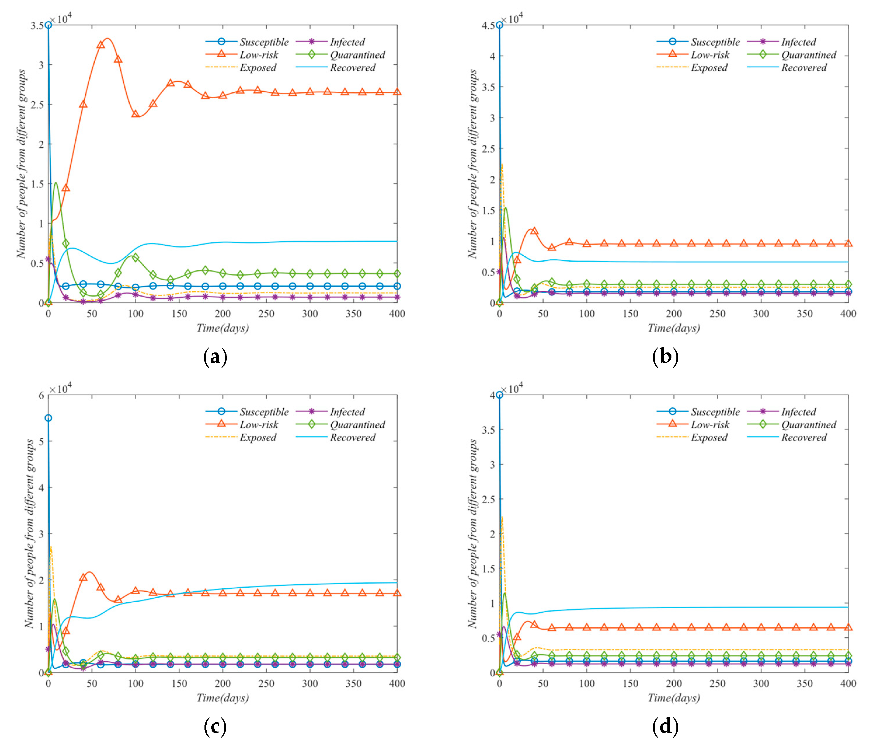
This example simulates the global stability of the equilibrium of endemic diseases with n = 4. The parameter values are set as γ₁ = 0.035, γ₂ = 0.040, γ₃ = 0.03, γ₄ = 0.045, and μ is reduced by one order of magnitude. The remaining parameters are listed in Table 1. Given these settings, R₀ = 7.9728 > 1. The initial data for each region and state are shown in

Table 4. Initial data of the endemic disease equilibrium in each region.

State Variable	Region 1	Region 2	Region 3	Region 4
S	35,000	45,000	55,000	40,000
L	0	0	0	0
E	5000	4500	5500	4000
I	5500	5000	5000	5500
Q	0	0	0	0
D	0	0	0	0
R	0	0	0	0

.

The evolution diagrams obtained from simulation based on these parameters are shown in Figure 4a–d, and the phase trajectory diagrams are shown in Figure 5a–d.

5.3. Impact of Migration Rate on the Number of Infected

In order to study the impact of population movement on disease transmission, the number of infected individuals with different migration rates is considered.

Table 5. Set the parameters for each region.

Parameter	Region 1	Region 2	Region 3	Region 4
ρ	0.4	0.45	0.5	0.55
Λ	1000	1200	1300	1200
μ	0.015	0.025	0.010	0.02
m	0.035	0.015	0.025	0.02
β	1.5 × 10−5	2.5 × 10−5	1.5 × 10−5	2.5 × 10−5
φ	1 × 10−5	1.5 × 10−5	2 × 10−5	3 × 10−5
λ	0.15	0.1	0.15	0.35
δ	0.025	0.02	0.035	0.025
η	0.004	0.0035	0.0025	0.0025
θ	0.025	0.035	0.035	0.02
γ	0.0035	0.004	0.003	0.0045
α	0.001	0.005	0.002	0.004
q	0.25	0.35	0.45	0.45

lists the parameter values. The initial data of the number of infected in each region are 5500, 5000, 5000, and 5500, respectively. We assume that the mobility of all populations in each region is equal, and AT = BT = CT = DT = ET = [p_ij]_{4 × 4}. Where i ≠ j, and i, j = 1, 2, 3, 4, with p_ii = 0, for i = 1, 2, 3, 4. When p_ij = p_ji, all regions are connected with the same mobility. The migration rates p_ij are set to 0.0005, 0.005, and 0.05, respectively, as shown in Figure 6.

As mobility increases, the peak number of infected rises in regions 1, 2, and 4, while it decreases in region 3. According to the parameters in Table 5, the basic reproduction numbers of regions 1 to 4 are approximately R₀₁ ≈ 2.32, R₀₂ ≈ 2.70, R₀₃ ≈ 10.02, and R₀₄ ≈ 5.97, indicating that region 3 is a high-outbreak area. As mobility increases, the overall basic reproduction number decreases from 8.97 to 4.49. Therefore, in a multi-regional model, increased population migration may disperse the infected from high-outbreak areas to other regions. If better public health measures are implemented in the target area, the overall basic reproduction number could be reduced. For instance, consider region 1. If its immigration rate exceeds its emigration rate (where p₁ = p_1j = 0.005 and p₂ = p_j1 = 0.0005, with i ≠ j and i, j = 1, 2, 3, 4), the number of infected in region 1 will increase, while decreasing in other regions. Therefore, an increase in the immigration rate of the population in a local region will increase the number of infected in that region. Conversely, if the immigration rate of region 1 is lower than its emigration rate (where p₁ = p_1j = 0.005 and p₂ = p_j1 = 0.05, with i ≠ j and i, j = 1, 2, 3, 4), the number of infected in region 1 will decrease, while increasing in other regions.

5.4. Parameter Sensitivity Analysis

Global sensitivity analysis can identify the parameters that have the most significant effect on model results. The global parameter sensitivity is explored by analyzing the interactions between parameters, which can reveal the dynamic relationships within complex systems and help understand the internal mechanisms of the model. In this paper, the global parameter sensitivity of the model is analyzed using Latin hypercube sampling and the partial rank correlation coefficient method. To simplify the analysis, we simulate the model with n = 1. The basic steps of the global parameter sensitivity analysis are described as follows:

• Sample generation.

First, the distribution of each parameter is sampled evenly by dividing the probability density function of the input parameter into intervals with equal area, ensuring a balanced representation of the parameter’s distribution. Assuming that there are M input parameters and each parameter is divided into N intervals, the sample matrix A has dimensions of N × M.

2.

A Monte Carlo simulation is performed on randomly paired samples.

Each column of the sample matrix is randomly shuffled to generate a sample set of different parameter combinations. Each row in the sample matrix represents an input set for one Monte Carlo simulation.

3.

Comparing samples with the simulated outputs.

The simulated outputs are added to the sample matrix, and all values are converted to ranks. Then, the PRCC (Partial Rank Correlation Coefficient) is calculated. The input parameters are X₁, X₂, …, X_M, while the output is Y, and the rank-transformed matrix is R (X₁), R (X₂), …, R (Y). The influence of other parameters is controlled using the following multiple linear regression model:

$$\begin{array}{l}R(X_i)={\beta }_0+{\beta }_{1}R(X_1)+{\beta }_{2}R(X_2)+\dots +{\beta }_{M}R(X_M)+{ϵ}_i\\ R(Y)={\gamma }_0+{\gamma }_{1}R(X_1)+{\gamma }_{2}R(X_2)+\dots +{\gamma }_{M}R(X_M)+\eta R(Y)\end{array}$$

(45)

The residuals ε_i and η are calculated, and the PRCC can be estimated by

$$PRCC={\displaystyle \frac{C\mathrm{ov}(R({\epsilon }_i),R(\eta ))}{\sqrt{Var(R({\epsilon }_i))\cdot Var(R(\eta ))}}}$$

(46)

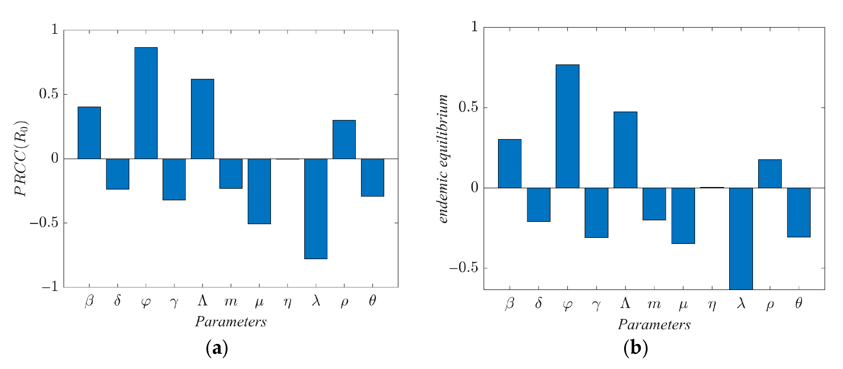
The PRCC value ranges from [–1, 1], where a larger absolute value indicates a more significant influence of the parameter on the output. According to the above analysis process, the sensitivity analysis of the global parameters for the R₀ and the endemic equilibrium can be obtained. The PRCC values for different parameters are shown in Figure 7.

According to the above results, the infection rate of susceptible subjects β_i and low-risk subjects φ_i in this model are positively correlated with the R₀ and the endemic equilibrium; i.e., as β_i and φ_i increase, the R₀ and the endemic equilibrium will increase. Similarly, the isolation rate λ_i and θ_i, and the recovery rate of infected γ_i are negatively correlated with the R₀ and the endemic equilibrium. Specifically, the φ_i, λ_i, θ_i, and γ_i show strong correlations with both the R₀ and the endemic equilibrium. Therefore, controlling the transmission rate of infectious diseases, isolating virus carriers, and improving medical care levels are essential strategies to prevent the spread of diseases. To verify the accuracy of global parameter sensitivity analysis results, a local parameter sensitivity analysis is performed for key parameters. Figure 8 illustrates the curves for parameters β, φ, λ, θ, and γ within their respective value ranges. The values of the other parameters are as follows: ρ = 0.4, Λ = 2000, μ = 0.15, δ = 0.2, η = 0.004, α = 0.1, and q = 0.25. The ranges of the remaining parameters are shown in

Table 6. Key parameters values for the infected.

Parameters	β	φ	λ	θ	γ	m
Data 1	[1.5–5.5] × 10−5	1 × 10−4	0.25	0.3	0.35	0.15
Data 2	1 × 10−4	[1.0–5.0] × 10−5	0.25	0.3	0.35	0.15
Data 3	1 × 10−4	1 × 10−4	[0.1–0.5]	0.3	0.35	0.15
Data 4	1 × 10−4	1 × 10−4	0.25	[0.1–0.5]	0.35	0.15
Data 5	1 × 10−4	1 × 10−4	0.25	0.3	[0.1–0.5]	0.15
Data 6	1 × 10−4	1 × 10−5	0.25	0.3	0.35	[0.1–0.5]

.

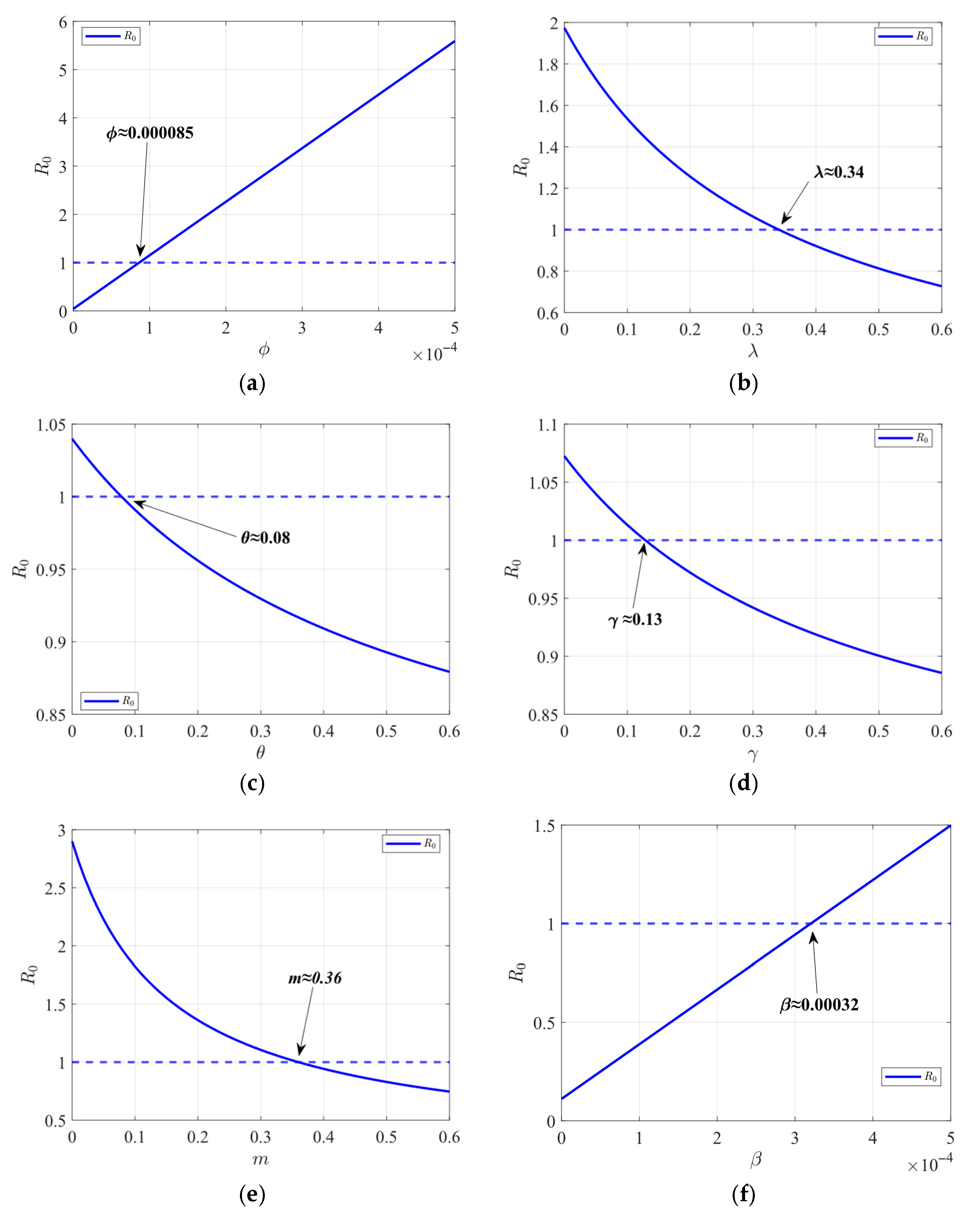
Furthermore, the sensitivity analysis for the R₀ is investigated. Data 1 to 6 in

Table 7. Key parameters for the R₀.

Parameters	β	φ	λ	θ	γ	m
Data 1	[0–5] × 10−4	1.0 × 10−5	0.25	0.3	0.35	0.15
Data 2	1.5 × 10−5	[0–5] × 10−4	0.25	0.3	0.35	0.15
Data 3	1.5 × 10−5	1.0 × 10−4	[0–0.6]	0.3	0.35	0.15
Data 4	1.5 × 10−5	8.0 × 10−5	0.25	[0–0.6]	0.35	0.15
Data 5	1.5 × 10−5	8.0 × 10−5	0.25	0.3	[0–0.6]	0.15
Data 6	5.0 × 10−4	1.0 × 10−5	0.25	0.3	0.35	[0–0.6]

show the value range of each group of parameters. The numerical simulation is shown in Figure 9. In Figure 9b,c, the value of R₀ increases with the infection rate β and φ. That means the increased infection rate can lead to an expansion of the epidemic. In contrast, Figure 9d–f indicate that the isolation rates of λ, θ, and γ have an inverse relationship with R₀. Therefore, enhancing the recovery rate and isolating virus carriers will effectively help prevent the spread of the epidemic.

Protection—Isolation Strategy Based on Optimal Path

In infectious disease dynamics, R₀ is a key epidemiological indicator that reflects the disease’s potential to spread. If R₀ < 1, disease transmission will gradually decline and eventually cease. Conversely, if R₀ > 1, infection may propagate within the population, potentially triggering a pandemic. The control of an epidemic can be analyzed by examining the association between R₀ and the threshold value of 1. In this paper, the protection rate m of S and the isolation rate λ of E are selected for analysis. These parameters are selected for analysis because β, φ, δ, and γ in the model are intrinsic epidemic traits; external factors have little impact on them. Therefore, we explore how protection measures and isolation strategies can effectively control the spread of disease by analyzing their influence on R₀.

Specifically, two parameters, m and λ, are selected to investigate the condition R (m, λ) = 1, where

$$\lambda ={\displaystyle \frac{\mathrm{\Lambda }(\phi (m+\mu )+\mu \rho (\beta -\phi )(\delta +\gamma +\eta +\theta ))}{\mu (m+\mu )(\gamma +\eta +\mu +\theta )}}-\mu -\delta$$

(47)

The parameters used in the simulation are as follows: ρ = 0.4, Λ = 1000, μ = 0.1, β = 0.0002, δ = 0.2, φ = 0.00002, η = 0.004, θ = 0.3, α = 0.1, q = 0.25, and γ = 0.35. The numerical simulation results are shown in Figure 10a. In this figure, the red curve intersects the plane where R (λ, m) = 1, dividing it into three regions (R₀ < 1, R₀ > 1, and R₀ = 1). When all other parameters remain constant, R0 reaches its maximum value in the absence of protective or isolation measures. As protective and isolation measures are gradually enhanced, the R0 moves from the R₀ > 1 region to the R₀ < 1 region, and the transmission of the epidemic tends to cease. Therefore, the optimal strategy is to implement the protection-quarantine strategy to cross the red curve as quickly as possible. From a geometric perspective, this corresponds to the optimal route OM starting at the origin and reaching the red curve. The coordinates M (λ₁, m₁) represent the optimal combination along this shortest path. The red curve equation in Figure 10b is

$$f(\lambda ,m)={\displaystyle \frac{\mathrm{\Lambda }(\phi (m+\mu )+\mu \rho (\beta -\phi )(\delta +\gamma +\eta +\theta ))}{\mu (m+\mu )(\gamma +\eta +\mu +\theta )(\delta +\mu +\lambda )}}-1$$

(48)

For the point M tangent vector $\overrightarrow{B}$, $\overrightarrow{OM}$⊥$\overrightarrow{B}$, where

$$\left\{\begin{array}{l}f({\lambda }_1,m_1)={\displaystyle \frac{\mathrm{\Lambda }(\phi (m_1+\mu )+\mu \rho (\beta -\phi )(\delta +\gamma +\eta +\theta ))}{\mu (m_1+\mu )(\gamma +\eta +\mu +\theta )(\delta +\mu +{\lambda }_1)}}-1=0\\ \left({\displaystyle \frac{-{\lambda }_1}{(\delta +\mu +{\lambda }_1)}}+{\displaystyle \frac{m_1}{(m_1+\mu )}}+{\displaystyle \frac{{\lambda }_1(\phi (m_1+\mu ))}{(\delta +\mu +{\lambda }_1)\mathrm{\Lambda }\mu \rho (\beta -\phi )(\delta +\gamma +\eta +\theta ))}}\right)\mathrm{\Delta }=0\\ \mathrm{\Delta }={\displaystyle \frac{\mathrm{\Lambda }\mu \rho (\beta -\phi )(\delta +\gamma +\eta +\theta ))}{\mu (m_1+\mu )(\gamma +\eta +\mu +\theta )(\delta +\mu +{\lambda }_1)}}\end{array}\right.$$

(49)

To prove the uniqueness of point M, it is only necessary to prove that the curve (50) is concave.

$$\left\{\begin{array}{l}\lambda ={\displaystyle \frac{\mathrm{\Lambda }(\phi (m+\mu )+\mu \rho (\beta -\phi ))(\delta +\gamma +\eta +\theta )}{\mu (m+\mu )(\gamma +\eta +\mu +\theta )}}-\delta -\mu \\ {\lambda }^{\prime \prime }={\displaystyle \frac{2\mathrm{\Lambda }AB}{C}}{\displaystyle \frac{1}{{(m+\mu )}^3}}\\ A=(\beta -\phi )\phi \rho \\ B=(\delta +\gamma +\eta +\theta )\\ C=\mu (\gamma +\eta +\mu +\theta )\end{array}\right.$$

(50)

Since the probability of a susceptible becoming infected is higher than that of a low-risk, and β-φ > 0, we have $> 0$. Therefore, the curve (50) is concave, Equation (49) has a unique solution, and a unique shortest path (λ₁, m₁) is obtained. If the protection intensity is λ₁ and the isolation intensity is m₁, the spread of the epidemic can be effectively controlled.

6. Conclusions

In this paper, on the basis of the traditional SEIR model, a SLEIQDR model of multi-regional population migration is established by combining the factors of population migration, low-risk individuals, and isolated individuals. First, the model’s uniqueness of the disease-free equilibrium is proved, the basic reproduction number is calculated, and the relationship between the single region and multiple regions is analyzed. Furthermore, a Lyapunov function is constructed to prove the stability of the endemic equilibrium and the disease-free equilibrium, and the correctness of the theory is proved by numerical analysis. To explore the impact of population migration on the number of infected, changes in infection numbers across different regions under varying migration rates are simulated. The results show that population migration facilitates the spread of the virus from high-infection areas to low-infection areas, exacerbating the situation in the latter. However, strong public health measures implemented in low-infection areas can effectively prevent the spread and reduce the overall basic reproduction number. In addition, the number of infected increases in areas where the immigration rate is greater than the emigration rate. Finally, a parameter sensitivity analysis is conducted for the single region case, and an optimal protection isolation strategy is proposed. The results indicate that increasing isolation and recovery rates, along with reducing the infection rate, will significantly reduce the spread of the disease. This study will help decision-makers better grasp the dynamics of the epidemic and optimize the response measures to effectively mitigate the epidemic’s impact on society. However, due to the complexity of the model, it is difficult to estimate its parameters with real datasets. Future work should focus on developing parameter estimation methods for this model and calibrating the model using real datasets.

References

1. López, L.; Giovanini, L. Adaptive dynamic social networks using an agent-based model to study the role of social awareness in infectious disease spread. Phys. D Nonlinear Phenom. 2025, 474, 134530. [Google Scholar] [CrossRef]
2. Deng, Y.; He, D.; Zhao, Y. Assessment of age-dependent effects during the transmission of Omicron and the outcomes of booster campaign vaccination strategies. Appl. Math. Model. 2024, 133, 148–169. [Google Scholar] [CrossRef]
3. Hwang, E. A partially periodic oscillation model combined with heterogeneous autoregression and its application to COVID-19. Appl. Math. Model. 2024, 125, 509–528. [Google Scholar] [CrossRef]
4. Njankou, S.D.D.; Nyabadza, F. Modelling the potential influence of human migration and two strains on Ebola virus disease dynamics. Infect. Dis. Model. 2022, 7, 645–659. [Google Scholar] [CrossRef]
5. Kar, S.; Maiti, D.K.; Maiti, A.P. HIV/AIDS control owing to local and global awareness, diagnosis, treatment tactics and control theory: Fractional order modeling. Nonlinear Dyn. 2024, 112, 22391–22420. [Google Scholar] [CrossRef]
6. Guo, W.; Zheng, B.; Yu, J. Modeling the dengue control dynamics based on a delay stochastic differential system. Comput. Appl. Math. 2024, 43, 166. [Google Scholar] [CrossRef]
7. Wu, B.; Huo, L. The influence of different government policies on the co-evolution of information dissemination, vaccination behavior and disease transmission in multilayer networks. Chaos Solitons Fractals 2024, 180, 114522. [Google Scholar] [CrossRef]
8. Kerkmann, D.; Korf, S.; Nguyen, K.; Abele, D.; Schengen, A.; Gerstein, C.; Göbbert, J.H.; Basermann, A.; Kühn, M.J.; Meyer-Hermann, M. Agent-based modeling for realistic reproduction of human mobility and contact behavior to evaluate test and isolation strategies in epidemic infectious disease spread. Comput. Biol. Med. 2025, 193, 110269. [Google Scholar] [CrossRef] [PubMed]
9. Alkhazzan, A.; Wang, J.; Nie, Y.; Khan, H.; Alzabut, J. A novel SIRS epidemic model for two diseases incorporating treatment functions, media coverage, and three types of noise. Chaos Solitons Fractals 2024, 181, 114631. [Google Scholar] [CrossRef]
10. Ali, I.; Khan, S.U. Analysis of stochastic delayed SIRS model with exponential birth and saturated incidence rate. Chaos Solitons Fractals 2020, 138, 110008. [Google Scholar] [CrossRef]
11. Yin, Q.; Wang, Z.; Xia, C. Information-epidemic co-evolution propagation under policy intervention in multiplex networks. Nonlinear Dyn. 2023, 111, 14583–14595. [Google Scholar] [CrossRef]
12. Centres, P.M.; Perez-Morelo, D.J.; Guzman, R.; Reinaudi, L.; Gimenez, M.C. Diffusion model for the spread of infectious diseases: SIR model with mobile agents. Phys. A Stat. Mech. Its Appl. 2024, 633, 129399. [Google Scholar] [CrossRef]
13. Song, X.; Peng, Z.; Song, S.; Stojanovic, V. Asynchronous state estimation for switched nonlinear reaction–diffusion SIR epidemic models with impulsive effects. Biomed. Signal Process. Control 2025, 105, 107600. [Google Scholar] [CrossRef]
14. El Khalifi, M.; Britton, T. SIRS epidemics with individual heterogeneity of immunity waning. J. Theor. Biol. 2024, 587, 111815. [Google Scholar] [CrossRef]
15. Guan, G.; Guo, Z.; Xiao, Y. Dynamical behaviors of a network-based SIR epidemic model with saturated incidence and pulse vaccination. Commun. Nonlinear Sci. Numer. Simul. 2024, 137, 108097. [Google Scholar] [CrossRef]
16. Aguiar, M.; Steindorf, V.; Srivastav, A.K.; Stollenwerk, N.; Kooi, B.W. Bifurcation analysis of a two infection SIR-SIR epidemic model with temporary immunity and disease enhancement. Nonlinear Dyn. 2024, 112, 13621–13639. [Google Scholar] [CrossRef]
17. Al-Darabsah, I. A time-delayed SVEIR model for imperfect vaccine with a generalized nonmonotone incidence and application to measles. Appl. Math. Model. 2021, 91, 74–92. [Google Scholar] [CrossRef]
18. Yu, Z.; Zhang, J.; Zhang, Y.; Cong, X.; Li, X.; Mostafa, A.M. Mathematical modeling and simulation for COVID-19 with mutant and quarantined strategy. Chaos Solitons Fractals 2024, 181, 114656. [Google Scholar] [CrossRef]
19. Chebotaeva, V.; Srinivasan, A.; Vasquez, P.A. Differentiating Contact with Symptomatic and Asymptomatic Infectious Individuals in a SEIR Epidemic Model. Bull. Math. Biol. 2025, 87, 38. [Google Scholar] [CrossRef]
20. Wang, Y.; Tu, L.; Wang, X.; Guo, Y. Evolutionary vaccination game considering intra-seasonal strategy shifts regarding multi-seasonal epidemic spreading. Chaos Solitons Fractals 2024, 180, 114419. [Google Scholar] [CrossRef]
21. Khairulbahri, M. The SEIR model incorporating asymptomatic cases, behavioral measures, and lockdowns: Lesson learned from the COVID-19 flow in Sweden. Biomed. Signal Process. Control 2023, 81, 104416. [Google Scholar] [CrossRef]
22. Yang, Z.; Zeng, Z.; Wang, K.; Wong, S.S.; Liang, W.; Zanin, M.; Liu, P.; Cao, X.; Gao, Z.; Mai, Z.; et al. Modified SEIR and AI prediction of the epidemics trend of COVID-19 in China under public health interventions. J. Thorac. Dis. 2020, 12, 165–174. [Google Scholar] [CrossRef]
23. Chen, Z.; Feng, L.; Lay, H.A., Jr.; Furati, K.; Khaliq, A. SEIR model with unreported infected population and dynamic parameters for the spread of COVID-19. Math. Comput. Simul. 2022, 198, 31–46. [Google Scholar] [CrossRef]
24. Das, T.; Srivastava, P.K.; Kumar, A. Nonlinear dynamical behavior of an SEIR mathematical model: Effect of information and saturated treatment. Chaos Interdiscip. J. Nonlinear Sci. 2021, 31, 043104. [Google Scholar] [CrossRef]
25. Luebben, G.; González-Parra, G.; Cervantes, B. Study of optimal vaccination strategies for early COVID-19 pandemic using an age-structured mathematical model: A case study of the USA. Math. Biosci. Eng. 2023, 20, 10828–10865. [Google Scholar] [CrossRef] [PubMed]
26. Wang, D.; Zhang, S.; Wang, L. Deep epidemiological modeling by black-box knowledge distillation: An accurate deep learning model for COVID-19. In Proceedings of the AAAI Conference on Artificial Intelligence, Virtual, 2–9 February 2021; Volume 35, pp. 15424–15430. [Google Scholar]
27. Tu, Y.; Hayat, T.; Hobiny, A.; Meng, X. Modeling and multi-objective optimal control of reaction-diffusion COVID-19 system due to vaccination and patient isolation. Appl. Math. Model. 2023, 118, 556–591. [Google Scholar] [CrossRef] [PubMed]
28. Policarpo, J.M.P.; Ramos, A.; Dye, C.; Faria, N.R.; Leal, F.E.; Moraes, O.J.S.; Parag, K.V.; Peixoto, P.S.; Buss, L.; Sabino, E.C.; et al. Scale-free dynamics of Covid-19 in a Brazilian city. Appl. Math. Model. 2023, 121, 166–184. [Google Scholar] [CrossRef] [PubMed]
29. Bhouri, M.A.; Costabal, F.S.; Wang, H.; Linka, K.; Peirlinck, M.; Kuhl, E.; Perdikaris, P. COVID-19 dynamics across the US: A deep learning study of human mobility and social behavior. Comput. Methods Appl. Mech. Eng. 2021, 382, 113891. [Google Scholar] [CrossRef]
30. Mustavee, S.; Agarwal, S.; Enyioha, C.; Das, S. A linear dynamical perspective on epidemiology: Interplay between early COVID-19 outbreak and human mobility. Nonlinear Dyn. 2022, 109, 1233–1252. [Google Scholar] [CrossRef]
31. Bekiros, S.; Kouloumpou, D. SBDiEM: A new mathematical model of infectious disease dynamics. Chaos Solitons Fractals 2020, 136, 109828. [Google Scholar] [CrossRef]
32. Wang, Z.; Carrasco-Teja, M.; Zhang, X.; Teichert, G.H.; Garikipati, K. System inference via field inversion for the spatio-temporal progression of infectious diseases: Studies of COVID-19 in Michigan and Mexico. Arch. Comput. Methods Eng. 2021, 28, 4283–4295. [Google Scholar] [CrossRef]
33. Brockmann, D.; Helbing, D. The hidden geometry of complex, network-driven contagion phenomena. Science 2013, 342, 1337–1342. [Google Scholar] [CrossRef]
34. Mahmood, M.; Amaral, A.V.R.; Mateu, J.; Moraga, P. Modeling infectious disease dynamics: Integrating contact tracing-based stochastic compartment and spatio-temporal risk models. Spat. Stat. 2022, 51, 100691. [Google Scholar] [CrossRef] [PubMed]
35. Jia, Q.; Li, J.; Lin, H.; Tian, F.; Zhu, G. The spatiotemporal transmission dynamics of COVID-19 among multiple regions: A modeling study in Chinese provinces. Nonlinear Dyn. 2022, 107, 1313–1327. [Google Scholar] [CrossRef] [PubMed]
36. Guo, Z.G.; Sun, G.Q.; Wang, Z.; Jin, Z.; Li, L.; Li, C. Spatial dynamics of an epidemic model with nonlocal infection. Appl. Math. Comput. 2020, 377, 125158. [Google Scholar] [CrossRef]
37. Alleman, T.W.; Rollier, M.; Vergeynst, J.; Baetens, J.M. A Stochastic Mobility-Driven spatially explicit SEIQRD COVID-19 model with VOCs, seasonality, and vaccines. Appl. Math. Model. 2023, 123, 507–525. [Google Scholar] [CrossRef]
38. Das, D.K.; Ghorai, S.; Banerjee, M. Spatio-temporal dynamics of an SIS model with nonlinear incidence and nonlocal disease transmission. Nonlinear Dyn. 2023, 111, 15591–15612. [Google Scholar] [CrossRef]
39. Wang, J.; Wu, S.L.; Huang, M.; Zhao, H. Spatial spread for a delayed and nonlocal foot-and-mouth disease model. Nonlinear Anal. Real World Appl. 2024, 76, 104006. [Google Scholar] [CrossRef]
40. Sun, G.; Jin, Z.; Mai, A. Dynamics of a two-patch SIR model with disease surveillance mediated infection force. Commun. Nonlinear Sci. Numer. Simul. 2024, 132, 107872. [Google Scholar] [CrossRef]
41. Wu, P.; Wang, X.; Wang, H. Spatial heterogeneity analysis for the transmission of syphilis disease in China via a data-validated reaction–diffusion model. Math. Biosci. 2024, 375, 109243. [Google Scholar] [CrossRef]
42. Wang, W.; Wang, X.; Wang, H. Spatial dynamics of a generalized cholera model with nonlocal time delay in a heterogeneous environment. J. Differ. Equ. 2024, 405, 103–150. [Google Scholar] [CrossRef]
43. Akuno, A.O.; Ramirez-Ramirez, L.L.; Mehta, C.; Krishnanunni, C.G.; Bui-Thanh, T.; Montoya, J.A. Multi-patch epidemic models with partial mobility, residency, and demography. Chaos Solitons Fractals 2023, 173, 113690. [Google Scholar] [CrossRef]
44. Zhao, G.; Ruan, S. Spatiotemporal dynamics in epidemic models with Lévy flights: A fractional diffusion approach. J. Mathématiques Pures Appliquées 2023, 173, 243–277. [Google Scholar] [CrossRef]
45. Gross, B.; Zheng, Z.; Liu, S.; Chen, X.; Sela, A.; Li, J.; Li, D.; Havlin, S. Spatio-temporal propagation of COVID-19 pandemics. Europhys. Lett. 2020, 131, 58003. [Google Scholar] [CrossRef]
46. He, S.; Peng, Y.; Sun, K. SEIR modeling of the COVID-19 and its dynamics. Nonlinear Dyn. 2020, 101, 1667–1680. [Google Scholar] [CrossRef]
47. Li, M.Y.; Shuai, Z. Global-stability problem for coupled systems of differential equations on networks. J. Differ. Equ. 2010, 248, 1–20. [Google Scholar] [CrossRef]
Figure 1. State transition diagram of the multi-region SLEIQDR model.
Technologies 13 00425 g001
Figure 2. Evolution diagram of disease-free equilibrium. (a) Evolution diagram of disease-free equilibrium in region 1; (b) evolution diagram of disease-free equilibrium in region 2; (c) evolution diagram of disease-free equilibrium in region 3; and (d) evolution diagram of disease-free equilibrium in region 4.
Technologies 13 00425 g002
Figure 3. Phase trajectory diagram of the disease-free equilibrium. (a) Phase trajectory diagram of disease-free equilibrium in region 1; (b) phase trajectory diagram of disease-free equilibrium in region 2; (c) phase trajectory diagram of disease-free equilibrium in region 3; and (d) phase trajectory diagram of disease-free equilibrium in region 4.
Technologies 13 00425 g003
Figure 4. Evolution diagram of the equilibrium of endemic diseases. (a) Evolution diagram of endemic disease equilibrium in region 1; (b) evolution diagram of endemic disease equilibrium in region 2; (c) evolution diagram of endemic disease equilibrium in region 3; and (d) evolution diagram of endemic disease equilibrium in region 4.
Technologies 13 00425 g004
Figure 5. Phase trajectory diagram of the endemic disease equilibrium. (a) Phase trajectory diagram of endemic disease equilibrium in region 1; (b) phase trajectory diagram of endemic disease equilibrium in region 2; (c) phase trajectory diagram of endemic disease equilibrium in region 3; and (d) phase trajectory diagram of endemic disease equilibrium in region 4.
Technologies 13 00425 g005
Figure 6. Number of infected under different mobility. (a) The changes in the number of infected in region 1 with different migration rates; (b) the changes in the number of infected in region 2 with different migration rates; (c) the changes in the number of infected in region 3 with different migration rates; and (d) the changes in the number of infected in region 4 with different migration rates.
Technologies 13 00425 g006
Figure 7. Sensitivity analysis of global parameters of R0 and endemic equilibrium; (a) sensitivity analysis of the global parameters for R0; (b) sensitivity analysis of the global parameters for the endemic equilibrium.
Technologies 13 00425 g007
Figure 8. Influence of different parameters on the number of infected. (a) sensitivity analysis of the number of infected with β; (b) sensitivity analysis of the number of infected with φ; (c) sensitivity analysis of the number of infected with λ; (d) sensitivity analysis of the number of infected with γ; (e) sensitivity analysis of the number of infected with θ; and (f) sensitivity analysis of the number of infected with m.
Technologies 13 00425 g008
Figure 9. Influence of different parameters on the basic reproduction number. (a) sensitivity analysis of R0 with φ; (b) sensitivity analysis of R0 with λ; (c) sensitivity analysis of R0 with θ; (d) sensitivity analysis of R0 with γ; (e) sensitivity analysis of R0 with m; and (f) sensitivity analysis of R0 with β.
Technologies 13 00425 g009
Figure 10. Basic reproduction number R0 distribution and optimal path diagram. (a) 3D graph of R0 distribution and optimal path; (b) Vertical view of R0 distribution and optimal path.
Technologies 13 00425 g010