Article

Workspace Definition in Parallelogram Manipulators: A Theoretical Framework Based on Boundary Functions

by
Luis F. Luque-Vega
1,
Jorge A. Lizarraga
2,
Dulce M. Navarro
2,
Jose R. Navarro
2,
Rocío Carrasco-Navarro
3,
Emmanuel Lopez-Neri
4,
Jesús Antonio Nava-Pintor
5,
Fabián García-Vázquez
5 and
Héctor A. Guerrero-Osuna
5,*
1
Department of Technological and Industrial Processes, ITESO, Tlaquepaque 45604, Jalisco, Mexico
2
Departamento de Investigación, Centro de Enseñanza Técnica Industrial, Guadalajara 44638, Jalisco, Mexico
3
Department of Mathematics and Physics, ITESO, Tlaquepaque 45604, Jalisco, Mexico
4
Centro de Investigación, Innovación y Desarrollo Tecnológico CIIDETEC-UVM, Universidad del Valle de México, Tlaquepaque 45601, Jalisco, Mexico
5
Unidad Académica de Ingeniería Eléctrica, Universidad Autónoma de Zacatecas, Zacatecas 98000, Zacatecas, Mexico
*
Author to whom correspondence should be addressed.
Technologies 2025, 13(9), 404; https://doi.org/10.3390/technologies13090404
Submission received: 31 May 2025 / Revised: 31 July 2025 / Accepted: 15 August 2025 / Published: 5 September 2025
(This article belongs to the Special Issue Collaborative Robotics and Human-AI Interactions)

Abstract

Robots with parallelogram mechanisms are widely employed in industrial applications due to their mechanical rigidity and precise motion control. However, the analytical definition of feasible workspace regions free from self-collisions remains an open challenge, especially considering the nonlinear and composite nature of such regions. This work introduces a mathematical model grounded in a collision theorem that formalizes boundary functions based on joint variables and geometric constraints. These functions explicitly define the envelope of safe configurations by evaluating relative positions between critical structural components. Using the MinervaBotV3 as a case study, the symbolic joint-space boundaries and their corresponding geometric regions in both 2D and 3D are computed and visualized. The feasible region is refined through centroid-based scaling to introduce safety margins and avoid singularities. The results show that this framework enables analytically continuous workspace representations, improving trajectory planning and reliability in constrained environments. Future work will extend this method to spatial mechanisms and real-time implementations in hybrid robotic systems.

1. Introduction

Manipulator robots are increasingly versatile, precise, and safe tools. These robots can perform extremely precise and repeatable movements, making them ideal for applications where accuracy is essential. Thanks to recent advances, they are now more adaptable and optimizable due to their advanced control algorithms, which enhance sustainability, facilitate the identification of imminent failures, and enable trajectory planning that allows them to efficiently adapt to unpredictable or unstructured environments.
However, each manipulator robot model has specific features that make it more suitable for certain types of applications. In particular, this work focuses on robots that incorporate parallelogram mechanisms within their structure. These linkages are widely used in industrial settings due to their ability to maintain orientation, enhance load-bearing capacity, and improve mechanical stiffness. At the same time, they introduce complex internal constraints and self-collision behaviors that are not easily captured by traditional workspace approximation techniques.
To illustrate the industrial relevance and structural diversity of this class of manipulators, Table 1 presents a representative set of commercial robots that feature embedded parallelogram mechanisms. This collection highlights key specifications such as payload, reach, degrees of freedom, and use-case context across different manufacturers and application domains.
For a more comprehensive understanding of these fundamental aspects, the Springer Handbook of Robotics, edited by Siciliano and Khatib [1], provides a detailed overview of modeling principles, kinematic analysis, trajectory planning, and control, becoming a key reference for the design and study of manipulator systems.
In this context, Gosselin and Jean [2] proposed an efficient algorithm to determine the actual workspace of planar parallel manipulators with three degrees of freedom, taking into account the physical limitations of both active and passive joints. Their method allows for accurate representations of the reachable area through the intersection of angular and circular regions, using Gauss’s Theorem to compute the workspace area at a low computational cost. This methodology has proven useful in the early stages of manipulator design and simulation.
On the other hand, recent research, such as that by Sisbot et al. [3], has emphasized the need to incorporate human–environment awareness into trajectory planning algorithms. In their study, mechanisms are proposed to adapt the motion of mobile manipulators in the presence of people, optimizing both safety and trajectory efficiency in shared, dynamic, and unstructured scenarios.
However, safety is a fundamental aspect for ensuring reliability in dynamic environments. This often requires integrating safety constraints into motion planning algorithms or adapting trajectories to avoid potential risks [4]. In this context, innovative methods have been developed, such as trajectory planning based on tree expansion using bubbles in the configuration space [5].
Furthermore, one of the most influential approaches in reactive planning is that proposed by Khatib [6], who introduced the potential fields method to achieve efficient real-time obstacle avoidance, allowing robots to generate dynamic trajectories in changing environments. On the other hand, traditional model-based detection methods in robotics focus primarily on the difference between estimated and actually applied torque [7]. Despite these advances, current methods still face challenges, such as high computational demand in some techniques and the need for more precise and expensive sensors to improve environmental perception.
In this regard, the concept of the “danger field” has emerged as a key indicator of risk in the robot’s vicinity [8].
An essential part of safe planning in manipulator robots is the correct delimitation of the workspace. To achieve effective delimitation, different approaches are used, among which danger fields and kinematic modeling simulations stand out. Knowing the actual available workspaces of manipulators is crucial in applications and design [9].
In this regard, Cao et al. [10] developed a method to efficiently evaluate the obstacle-free reachable workspace of industrial robots, enabling the identification of safe and operable regions with greater precision, contributing to more robust planning in real environments.
By integrating this information into planning algorithms, it is possible to adapt trajectories, allowing robots to operate more safely in complex environments. Moreover, knowing the actual available workspaces of manipulators is crucial in applications and design [11]. A well-defined workspace not only minimizes the risk of accidents but also optimizes the robot’s performance and adaptability in its tasks.
Furthermore, the integration of advanced sensors and artificial intelligence techniques, such as machine learning, has enabled manipulator robots to make real-time adjustments, optimizing their performance in dynamic scenarios.
Among these proposals, the work by Flacco et al. [12] stands out. They developed a reactive safety method based on depth sensors and kinematic models, enabling efficient evasive behaviors in response to potential collisions in industrial environments.
Likewise, Pham and Afify [13] conducted an extensive review of machine learning techniques and their applicability in intelligent manufacturing processes, highlighting their potential to improve the performance of robotic systems in changing environments through classification, prediction, and adaptive control.
Although there are methods where collision detection focuses on discrete collision prediction to avoid interferences [14], these methods often face high computational demands and challenges in unpredictable environments. However, current trends point toward the development of hybrid solutions that combine data-driven models with analytical approaches to improve the efficiency and accuracy of these systems.
Despite significant technological and design advances, the ability of manipulator robots to effectively interact with dynamic and unstructured environments remains a major technical barrier. While advanced planning algorithms have proven effective in controlled environments, their implementation in unpredictable scenarios, such as spaces shared with humans or moving objects, continues to be a considerable challenge. This is partly due to the need for real-time processing, which allows trajectories to be adjusted in response to sudden changes in the environment, often requiring high-performance hardware and optimized software, thus increasing implementation costs [15].
These limitations not only affect their ability to operate optimally but also highlight the need for further research and development. Although manipulators have improved in terms of energy optimization, in scenarios with multiple dynamic obstacles and dense trajectories, performance can degrade due to computational complexity [16].
Additionally, another significant challenge lies in the integration of next-generation sensors and actuators. Although advanced sensors, such as LiDAR systems, 3D cameras, and haptic sensors, improve robot perception and precision, their complexity and cost represent barriers to widespread adoption. Moreover, the data generated by these sensors require intensive processing and analysis, adding an additional layer of technical and computational complexity.
On the other hand, hydraulic manipulators—which are essential for high-force and high-resistance applications—present their own limitations. Despite their ability to handle heavy loads, their energy efficiency remains a persistent challenge. The inherent losses in the hydraulic system, along with the need for frequent maintenance, reduce their viability in applications where sustainability and energy efficiency are priorities [17].
Regarding the Denavit–Hartenberg (D-H) method, although it is widely used to represent manipulator configurations, it has important limitations. This approach is more complex than others due to the greater number of parameters and reference frames it handles. While it is more suitable for closed mechanisms and hybrid structures, it is not as efficient for simple open chains [18].
Another method is the pseudo-inverse of the Jacobian matrix, which—despite being widely used for its mathematical simplicity and applicability in known models—also has important limitations. Its open-loop nature leads to the accumulation of position errors over time, which restricts its effectiveness in long-duration tasks. Additionally, methods that rely on known models lack portability between robots with different parameters or structures [19].

2. Materials and Methods

This section introduces the mathematical framework used to define feasible regions in the joint space of a manipulator. A joint boundary function is formulated as a scalar condition on the joint variables, systematically delimiting the feasible configurations. Different types of joint boundary functions are classified according to the physical origin of the constraint, whether based on joint limits, geometric restrictions, or internal collisions.
Definition 1 (Joint Boundary Function). 
Let W q R n denote the feasible joint workspace, and let q R n represent the vector of joint variables. A joint boundary function β ( q ) : R n R is a scalar function defined such that:
β ( q ) = 0 , i f q W q , > 0 , i f q W q , < 0 , i f q W q .
All joint boundary functions are formulated and evaluated exclusively in the joint space. However, their effects are reflected in the feasible geometric workspace W g R 3 through the direct kinematic mapping
p = f ( q ) ,
where p denotes the geometric configuration associated with q . Consequently, constraints imposed in the joint space indirectly delimit the corresponding regions in the geometric space.
The primary purpose of a joint boundary function is to characterize the feasibility of a given configuration by detecting the occurrence of internal collisions or non-feasible configurations. In its most fundamental form, a collision is considered between two rigidly attached points, denoted as a + n and b + m , where a and b are principal frames along the kinematic chain 0 a a + n b b + m , and n, m are local point indices relative to their respective frames. A collision occurs if and only if the relative vector between these points vanishes:
r a + n , b + m = 0 ,
or equivalently, if the norm of the relative vector is null:
r a + n , b + m = 0 .
This fundamental notion is generalized in the construction of joint boundary functions, where scalar conditions are systematically formulated to ensure collision-free and feasible operation, regardless of whether the constraint originates from joint limits, geometric boundaries, or internal structural interactions.
To facilitate the interpretation of the mathematical framework and maintain clarity throughout the derivations, Table 2 summarizes the notation used in this section, including vectorial, kinematic, and geometric elements.

2.1. Link Boundary Functions

Link boundary functions represent a general class of constraints that analytically detect collisions between pairs of points rigidly attached to links of a kinematic chain. These functions evaluate the spatial proximity between the global positions of such points, expressed as recursive transformations from a common reference frame. A collision occurs when the Euclidean distance between these two global points vanishes.
To ensure clarity in notation, vectors in R 3 will be represented as r , while rotation matrices in R 3 × 3 will be denoted as R. Subscripts follow the convention that r i , j denotes the position vector of the point or frame j expressed in the coordinate system of frame i, and R i , j is the rotation matrix that transforms coordinates from frame j to frame i.
Let the general kinematic transformations for each link be defined as:
r 0 , 2 = r 0 , 1 + R 0 , 1 r 1 , 2 , R 0 , 2 = R 0 , 1 R 1 , 2 , r 0 , 2 = r 0 , 1 + R 0 , 1 r 1 , 2 , R 0 , 2 = R 0 , 1 R 1 , 2 .
Assume two points n and m defined locally in frames 2 and 2 , respectively. Their global positions are:
r 0 , n = r 0 , 2 + R 0 , 2 r 2 , n , r 0 , m = r 0 , 2 + R 0 , 2 r 2 , m ,
so that the relative vector is:
r n , m = r 0 , n r 0 , m = r 0 , 2 + R 0 , 2 r 2 , n r 0 , 2 R 0 , 2 r 2 , m .
Expanding both terms from their respective roots r 0 , 1 and r 0 , 1 , the full expression becomes:
β ( q ) = r 0 , 1 + R 0 , 1 r 1 , 2 + R 0 , 1 R 1 , 2 r 2 , n r 0 , 1 R 0 , 1 r 1 , 2 R 0 , 1 R 1 , 2 r 2 , m .
This expression can also be generalized to arbitrary depths:
β ( q ) = r n 3 , n 2 + R n 3 , n 2 r n 2 , n 1 + R n 3 , n 2 R n 2 , n 1 r n 1 , n r m 3 , m 2 R m 3 , m 2 r m 2 , m 1 R m 3 , m 2 R m 2 , m 1 r m 1 , m .
Alternatively, the function may be abstractly expressed as:
β ( q ) = r 0 , n r 0 , m ,
with the condition r 0 , m = r 0 , 0 + r 0 , m when both chains are expressed from a single base.
While this general formulation is mathematically complete and expressive, it is computationally expensive, particularly in robots with many degrees of freedom or deeply nested chains. Its evaluation requires full expansion of both kinematic branches, as well as explicit transformations through potentially long transformation sequences.
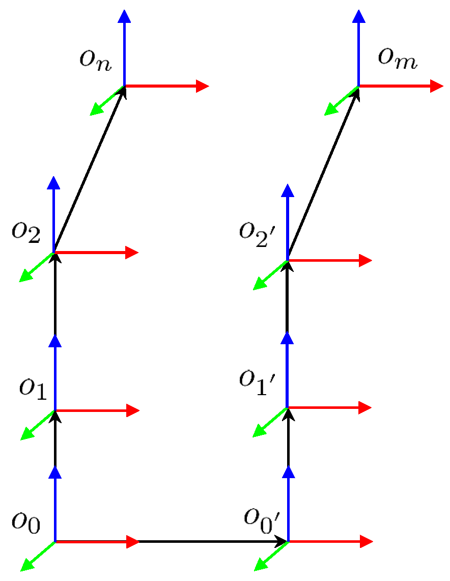
A diagram summarizing this general construction is shown in Figure 1, which illustrates the propagation of transformations from two distinct reference paths converging at a collision condition.
Given the high computational cost associated with the general formulation, it becomes necessary to identify structurally simplified expressions that are better suited for practical implementation. These simplifications exploit the topology of the kinematic chain to reduce the number of transformations, dimensional complexity, or depth of recursion, depending on the specific configuration under analysis.
Note that this approach facilitates a straightforward implementation of collision checks and the definition of boundaries, which are critical in the modeling of feasible workspaces and the optimization of manipulator trajectories. A significant simplification is achieved in the analysis of relative kinematic chains by avoiding the inherent complexity associated with homogeneous transformations and the Denavit–Hartenberg (DH) formalism. By focusing exclusively on the geometric relationships between consecutive systems, the need for complete transformation matrices is eliminated. Consequently, a more intuitive and computationally efficient model is provided, which is particularly advantageous in scenarios requiring rapid calculations and analytical clarity.
Two of these simplified cases, non-consecutive and consecutive link boundary functions, were originally introduced in [20]. In that work, collision conditions between local points on different links were formalized using recursive kinematics referenced from a common base frame. The approach demonstrated that the analytical evaluation of geometric coincidence is feasible and efficient under specific structural assumptions.
Building upon that foundation, the present formulation extends the modeling framework to more general topologies, including configurations with branching and symmetric bifurcations. As a result, four distinct types of link boundary functions are identified, each representing a situational simplification of the general model:
  • Collisions between non-consecutive links within a serial chain;
  • Collisions between directly connected consecutive links;
  • Collisions across distinct branches with non-coincident bifurcation offsets;
  • Collisions in bifurcated structures with coinciding geometric offsets.
The following sections present each of these cases, providing their corresponding analytical expression, kinematic assumptions, and diagrammatic interpretation.

2.2. Non-Consecutive Link Boundary Functions

This class of link boundary functions constitutes a situational simplification of the general model. It models collisions between two points n and m that belong to non-consecutive links of the same kinematic chain, both descending from a common ancestor frame. Instead of expanding both branches independently from the global base, the formulation restricts the propagation of transformations to the first shared frame in the kinematic hierarchy that connects both links. This allows the relative position to be constructed analytically and compactly within the common subtree, considerably reducing the computational complexity while preserving the rigor of the collision condition.
Let the chain be defined by the recursive transformations:
r 0 , 2 = r 0 , 1 + R 0 , 1 r 1 , 2 , R 0 , 2 = R 0 , 1 R 1 , 2 , r 0 , 3 = r 0 , 2 + R 0 , 2 r 2 , 3 , R 0 , 3 = R 0 , 2 R 2 , 3 , r 0 , 4 = r 0 , 3 + R 0 , 3 r 3 , 4 , R 0 , 4 = R 0 , 3 R 3 , 4 .
Assume the collision points are defined locally as r 2 , n in frame 2, and r 4 , m in frame 4. Their global positions are:
r 0 , n = r 0 , 2 + R 0 , 2 r 2 , n , r 0 , m = r 0 , 4 + R 0 , 4 r 4 , m ,
so that the relative vector is:
r n , m = r 0 , n r 0 , m = r 0 , 2 + R 0 , 2 r 2 , n r 0 , 4 + R 0 , 4 r 4 , m .
Using recursive substitution from r 0 , 1 , we expand:
r n , m = r 0 , 1 + R 0 , 1 r 1 , 2 + R 0 , 1 R 1 , 2 r 2 , n r 0 , 1 + R 0 , 1 r 1 , 2 + R 0 , 1 R 1 , 2 r 2 , 3 + R 0 , 1 R 1 , 2 R 2 , 3 r 3 , 4 + R 0 , 1 R 1 , 2 R 2 , 3 R 3 , 4 r 4 , m ,
which simplifies to:
r n , m = r 2 , n r 2 , 3 R 2 , 3 r 3 , 4 R 2 , 3 R 3 , 4 r 4 , m r n , m = 0 .
Thus, the corresponding scalar boundary function is:
β ( q ) = r 2 , n r 2 , 3 R 2 , 3 r 3 , 4 R 2 , 3 R 3 , 4 r 4 , m .
In a generalized notation, for any two points n and m defined in non-consecutive frames a and b, expressed via a shared upstream frame a, the function can be expressed as:
β ( q ) = r a , n r a , b 1 R a , b 1 r b 1 , b R a , b 1 R b 1 , b r b , m .
This structure is particularly relevant in robotic systems with serial chains or articulated arms, where links that are not directly connected may still enter into collision due to their motion. Analytical detection of such scenarios ensures safe path planning without resorting to computationally intensive geometric checks.
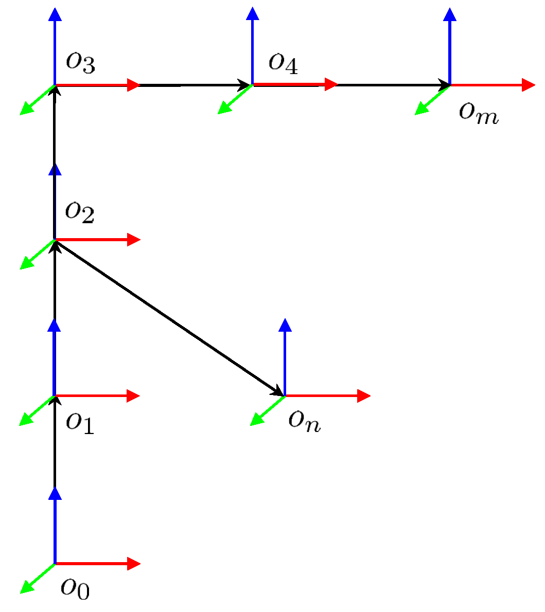
A graphical representation of this configuration is shown in Figure 2, which illustrates the recursive propagation of positions and orientations and highlights the collision points n and m on non-adjacent links.

2.3. Consecutive Link Boundary Functions

This case represents a direct simplification of the general model, applicable when both collision points n and m belong to consecutive links of the kinematic chain. The expressions involved are simplified due to the direct adjacency of the associated frames, which allows the relative position to be computed entirely within a local reference chain. As a result, the boundary function can be formulated in terms of a minimal recursive segment, without the need to propagate transformations from the global base or traverse additional joints. This structure significantly reduces computational complexity while retaining analytical precision.
Let the forward kinematics be defined as:
r 0 , 2 = r 0 , 1 + R 0 , 1 r 1 , 2 , R 0 , 2 = R 0 , 1 R 1 , 2 , r 0 , 3 = r 0 , 2 + R 0 , 2 r 2 , 3 , R 0 , 3 = R 0 , 2 R 2 , 3 ,
and consider two points n and m, fixed in frames 2 and 3, respectively. Their global positions are:
r 0 , n = r 0 , 2 + R 0 , 2 r 2 , n , r 0 , m = r 0 , 3 + R 0 , 3 r 3 , m .
The relative vector is given by:
r n , m = r 0 , n r 0 , m = r 0 , 2 + R 0 , 2 r 2 , n r 0 , 3 + R 0 , 3 r 3 , m ,
which simplifies as:
r n , m = r 0 , 2 + R 0 , 2 r 2 , n r 0 , 3 R 0 , 3 r 3 , m .
Expanding all terms from the common origin r 0 , 1 , we obtain:
r n , m = r 0 , 1 + R 0 , 1 r 1 , 2 + R 0 , 1 R 1 , 2 r 2 , n r 0 , 1 + R 0 , 1 r 1 , 2 + R 0 , 2 r 2 , 3 + R 0 , 1 R 1 , 2 R 2 , 3 r 3 , m ,
which reduces to:
r n , m = r 2 , n r 2 , 3 R 2 , 3 r 3 , m r n , m = 0 .
The scalar boundary function is then defined as:
β ( q ) = r 2 , n r 2 , 3 R 2 , 3 r 3 , m .
In general form, for any two points n and m located in consecutive frames a and b, the expression becomes:
β ( q ) = r a , n r a , b R a , b r b , m .
This formulation directly evaluates the spatial distance between the two points when expressed in a shared reference frame, and a collision is detected when the function evaluates to zero. Its simplicity and analytical clarity make it highly suitable for real-time implementations in trajectory validation and control.
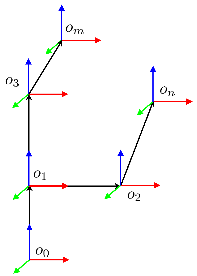
A graphical representation of the kinematic configuration involved in these expressions is shown in Figure 3, where the recursive construction of positions and orientations is depicted along with the locations of the points n and m on their respective links.

2.4. Branched Link Boundary Functions

This type of boundary function applies when the collision points n and m are located on two distinct branches of a kinematic chain that diverge from a common ancestor frame. These branches are not sequentially connected but share the same origin in the tree structure, typically at frame a 1 = b 1 . This formulation simplifies the general model by anchoring both branches to that bifurcation point, allowing each point to be propagated independently along its respective branch. Since both expressions share the same upstream root, there is no need to expand the transformations from the global base, making this a structurally efficient simplification of the full model.
Let the kinematics be defined as:
r 0 , 2 = r 0 , 1 + R 0 , 1 r 1 , 2 , R 0 , 2 = R 0 , 1 R 1 , 2 , r 0 , 3 = r 0 , 1 + R 0 , 1 r 1 , 3 , R 0 , 3 = R 0 , 1 R 1 , 3 ,
and the points n and m are locally defined in frames 2 and 3, respectively. Their global positions are:
r 0 , n = r 0 , 2 + R 0 , 2 r 2 , n , r 0 , m = r 0 , 3 + R 0 , 3 r 3 , m ,
so the relative position vector is:
r n , m = r 0 , n r 0 , m = r 0 , 2 + R 0 , 2 r 2 , n r 0 , 3 + R 0 , 3 r 3 , m .
Expanding all terms with respect to the common origin r 0 , 1 , we have:
r 0 , n = r 0 , 1 + R 0 , 1 r 1 , 2 + R 0 , 1 R 1 , 2 r 2 , n , r 0 , m = r 0 , 1 + R 0 , 1 r 1 , 3 + R 0 , 1 R 1 , 3 r 3 , m ,
so that:
r n , m = r 1 , 2 + R 1 , 2 r 2 , n r 1 , 3 R 1 , 3 r 3 , m r n , m = 0 .
This leads to the scalar boundary function:
β ( q ) = r 1 , 2 + R 1 , 2 r 2 , n r 1 , 3 R 1 , 3 r 3 , m .
More generally, when the bifurcation occurs at a common frame a 1 = b 1 , and the two branches extend to frames a and b, the boundary function can be expressed as:
β ( q ) = r a 1 , a + R a 1 , a r a , n r a 1 , b R a 1 , b r b , m .
Alternatively, by expressing both branches from the same node b 1 = a 1 , the equivalent form is:
β ( q ) = r b 1 , a + R b 1 , a r a , n r b 1 , b R b 1 , b r b , m .
This case is particularly important in delta-like mechanisms, dual-arm robots, or modular configurations where multiple kinematic chains originate from a shared base and may cross paths. The evaluation of such constraints allows the analytical detection of cross-branch collisions within a common reference structure.
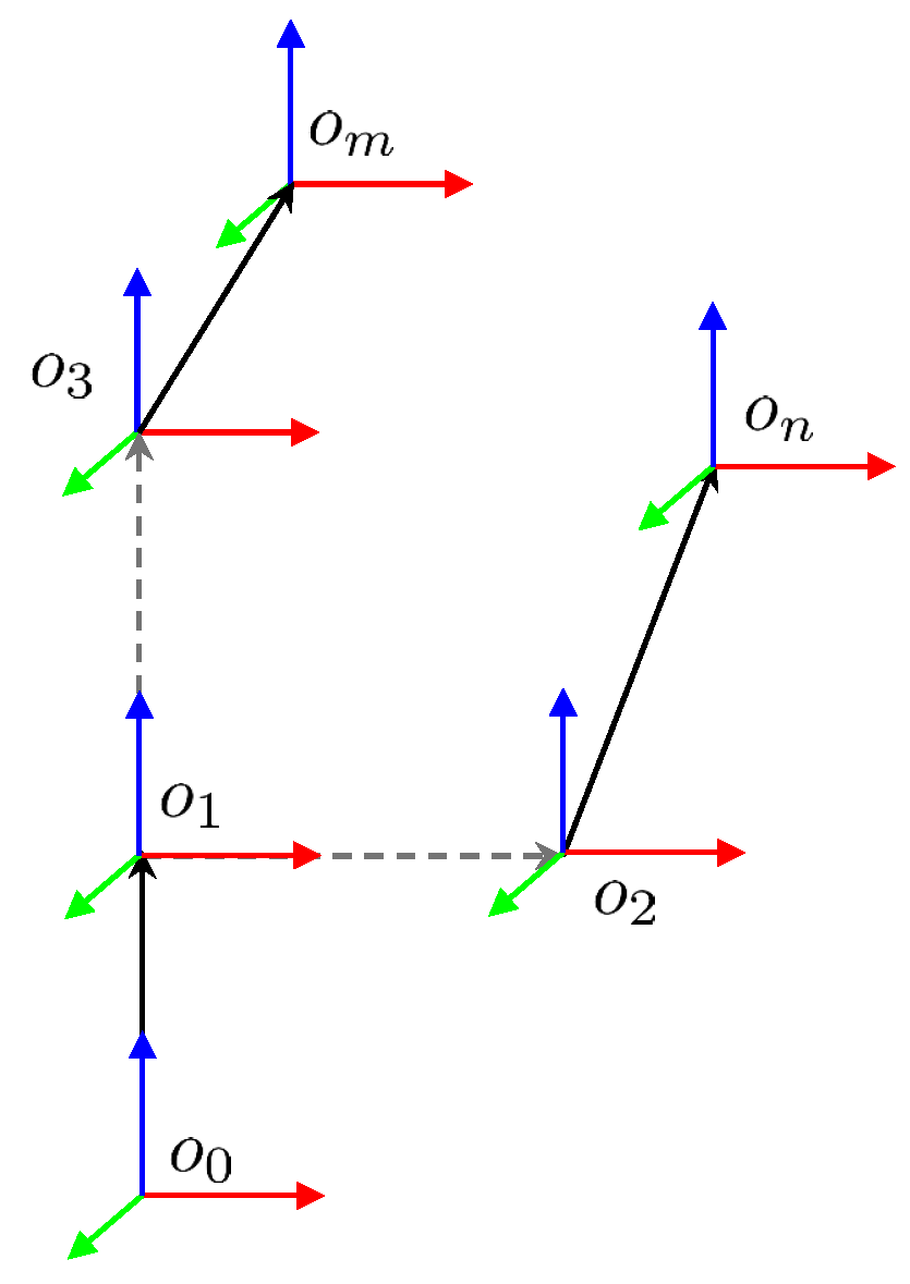
A diagram illustrating this bifurcated kinematic configuration is provided in Figure 4, which highlights the propagation of frames and the computation of the boundary function between branches.

2.5. Coincident Branched Link Boundary Functions

This case corresponds to collision detection between two points located on separate branches of a kinematic chain that diverge from a common frame a 1 = b 1 , where the spatial offsets from the bifurcation node to each branch are equal. This is the most compact of the boundary function types derived from the general model, as the coincidence of both branches in position and origin causes the relative position between them to depend solely on the internal geometry and local orientations. As a result, the general formulation collapses into a purely rotational comparison, significantly simplifying the analytical expression and reducing its computational cost.
Let the transformations be defined as:
r 0 , 2 = r 0 , 1 + R 0 , 1 r 1 , 2 , R 0 , 2 = R 0 , 1 R 1 , 2 , r 0 , 3 = r 0 , 1 + R 0 , 1 r 1 , 3 , R 0 , 3 = R 0 , 1 R 1 , 3 ,
and the global positions of points n and m are given by:
r 0 , n = r 0 , 2 + R 0 , 2 r 2 , n , r 0 , m = r 0 , 3 + R 0 , 3 r 3 , m .
Thus, the relative vector is:
r n , m = r 0 , n r 0 , m = r 0 , 2 + R 0 , 2 r 2 , n r 0 , 3 + R 0 , 3 r 3 , m .
Expanding both terms from r 0 , 1 , we have:
r n , m = r 0 , 1 + R 0 , 1 r 1 , 2 + R 0 , 1 R 1 , 2 r 2 , n r 0 , 1 + R 0 , 1 r 1 , 3 + R 0 , 1 R 1 , 3 r 3 , m ,
which simplifies to:
r n , m = R 0 , 1 r 1 , 2 + R 1 , 2 r 2 , n r 1 , 3 R 1 , 3 r 3 , m .
Now, under the condition r 1 , 2 = r 1 , 3 , we obtain:
r n , m = R 0 , 1 R 1 , 2 r 2 , n R 1 , 3 r 3 , m r n , m = 0 .
This yields the scalar boundary function:
β ( q ) = R 1 , 2 r 2 , n R 1 , 3 r 3 , m .
In general notation, where a 1 = b 1 is the bifurcation node, the function can be expressed as:
β ( q ) = R a 1 , a r a , n R a 1 , b r b , m = R b 1 , a r a , n R b 1 , b r b , m .
This formulation is particularly efficient in parallel robots or mirrored arms where structural symmetry leads to coinciding offsets, and only the relative orientations determine proximity. A diagram illustrating this symmetric bifurcation case is shown in Figure 5.

3. Results and Discussion

To illustrate the practical application of the boundary function framework developed in this work, a case study is conducted using the MinervaBotV3 platform. This robot was selected as a representative model because its structure and kinematic configuration naturally exhibit all four types of link boundary functions: consecutive, non-consecutive, branched non-coincident, and branched coincident. Such diversity makes it an ideal testbed for evaluating and validating the analytical formulations presented in the previous sections, as it enables comprehensive exploration of internal collisions arising from multiple structural relationships.
The MinervaBotV3 is a robotic manipulator developed for educational purposes at CETI Colomos. It serves as a palletizing robot with three degrees of freedom: q 1 , representing a rotation about the z-axis, and q 2 and q 3 , representing rotations about the y-axis. Figure 6 provides an isometric view of the robot, illustrating its geometric configuration and joint arrangement.
This robot serves as a practical platform for demonstrating concepts in robotics education, with a focus on trajectory planning and workspace analysis. To define the feasible workspace of MinervaBotV3, its geometric parameters, constraints, and self-collision criteria are considered, as described in Table 3. The direct kinematics equations, detailed in Table 4, are expressed recursively to provide a comprehensive understanding of the manipulator’s motion and positional relationships.
The kinematic chain of MinervaBotV3, illustrated in Figure 7, provides a detailed representation of the relative positions and rotational axes of its joints. The degrees of freedom are described as follows:
  • q 1 : Represents a rotational motion about the z-axis at the base.
  • q 2 : Represents a rotation about the y-axis at the second joint, allowing vertical adjustments.
  • q 3 : Represents an additional y-axis rotation to enhance the flexibility of the end-effector’s positioning.
Figure 7. Representation of the kinematic chain for MinervaBotV3.
Technologies 13 00404 g007

3.1. Boundary Functions for Workspace Definition

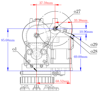
To formally define the collision-free workspace of the MinervaBotV3, a set of ten boundary functions β i ( q ) is introduced. Each function evaluates the relative position of key components within the manipulator’s structure, capturing potential self-collision scenarios across both consecutive links and branched subchains.
The notation β i ( q ) denotes the vector-valued boundary function associated with the i-th constraint. Each of these functions can be decomposed into three scalar components β i , j ( q ) , where the second subscript j { 1 , 2 , 3 } corresponds to the Cartesian coordinates x, y, and z, respectively, within the chosen reference frame. A contact or collision condition is identified when all components simultaneously vanish, i.e., β i , 1 = β i , 2 = β i , 3 = 0 , indicating spatial coincidence between the evaluated points.
In the case of planar mechanisms such as the MinervaBotV3, motion is constrained to the x z -plane. As a result, the component β i , 2 ( q ) , corresponding to the y-axis, is identically zero by construction and thus omitted in the scalar analysis. Therefore, only β i , 1 ( q ) and β i , 3 ( q ) are considered relevant in practice. These represent the horizontal and vertical displacements, respectively, between pairs of points under evaluation.
This scalar decomposition enables compact formulation and facilitates the computation of analytical bounds, which are subsequently used to define the feasible joint-space region.
Table 5, Table 6, Table 7, Table 8, Table 9, Table 10, Table 11, Table 12, Table 13 and Table 14 summarize the complete formulation of these constraints. For each case, the geometric configuration of the involved frames is depicted alongside the corresponding analytical expression of the boundary function.
The first three cases (Table 5, Table 6 and Table 7) correspond to collisions between consecutive links, where one frame is defined in the local system of a link and the other in the next one along the kinematic chain. Each boundary function measures the Euclidean distance between the transformed positions of the two points in a common frame.
Table 8, Table 9, Table 10 and Table 11 present boundary functions associated with branched-link interactions, where components from distinct kinematic branches are expressed in a shared reference frame to evaluate possible intersections. These scenarios typically arise from mechanical structures with parallelogram-like symmetry or alternative motion paths.
The remaining cases (Table 12, Table 13 and Table 14) revisit consecutive link interactions but in configurations closer to the robot’s base or terminal branches, reinforcing the generality of the formulation across the full manipulator structure.
All expressions incorporate rotation matrices and displacement vectors derived from the robot’s recursive kinematic model. A collision is considered to occur if and only if the corresponding norm of the boundary function evaluates to zero:
β i ( q ) = 0 r a r b = 0
ensuring that the involved points are coincident in space.
This formalism enables the systematic detection of constraint-violating configurations and supports the derivation of a feasible joint-space region for trajectory planning, as explored in subsequent sections.
From the individual formulations detailed in Table 5, Table 6, Table 7, Table 8, Table 9, Table 10, Table 11, Table 12, Table 13 and Table 14, it is possible to isolate the scalar components β i , 1 and β i , 3 for each boundary function β i ( q ) . These components correspond to the horizontal and vertical distances, respectively, between the evaluated points within the selected reference frame. By aggregating these expressions, the entire boundary constraint system can be compactly expressed as the following vector-valued function:
β 1 , 1 β 1 , 3 β 2 , 1 β 2 , 3 β 3 , 1 β 3 , 3 β 4 , 1 β 4 , 3 β 5 , 1 β 5 , 3 β 6 , 1 β 6 , 3 β 7 , 1 β 7 , 3 β 8 , 1 β 8 , 3 β 9 , 1 β 9 , 3 β 10 , 1 β 10 , 3 = x 2 , 7 x 3 , 8 cos ( q 2 q 3 ) + z 3 , 8 sin ( q 2 q 3 ) z 2 , 7 z 2 , 3 z 3 , 8 cos ( q 2 q 3 ) x 3 , 8 sin ( q 2 q 3 ) x 2 , 9 x 3 , 10 cos ( q 2 q 3 ) + z 3 , 10 sin ( q 2 q 3 ) z 2 , 9 z 2 , 3 z 3 , 10 cos ( q 2 q 3 ) x 3 , 10 sin ( q 2 q 3 ) x 3 , 11 x 3 , 4 x 4 , 12 cos ( q 3 ) + z 4 , 12 sin ( q 3 ) z 3 , 11 z 3 , 4 z 4 , 12 cos ( q 3 ) x 4 , 12 sin ( q 3 ) x 2 , 14 cos ( q 2 ) x 13 , 15 cos ( q 3 ) z 13 , 15 sin ( q 3 ) + z 2 , 14 sin ( q 2 ) z 2 , 14 cos ( q 2 ) z 13 , 15 cos ( q 3 ) + x 13 , 15 sin ( q 3 ) x 2 , 14 sin ( q 2 ) x 3 , 17 cos ( q 2 q 3 ) x 16 , 18 cos ( q 3 ) z 16 , 18 sin ( q 3 ) z 3 , 17 sin ( q 2 q 3 ) x 16 , 18 sin ( q 3 ) z 16 , 18 cos ( q 3 ) + z 3 , 17 cos ( q 2 q 3 ) + x 3 , 17 sin ( q 2 q 3 ) x 3 , 20 cos ( q 2 q 3 ) x 16 , 21 cos ( q 3 ) z 16 , 21 sin ( q 3 ) z 3 , 20 sin ( q 2 q 3 ) x 16 , 21 sin ( q 3 ) z 16 , 21 cos ( q 3 ) + z 3 , 20 cos ( q 2 q 3 ) + x 3 , 20 sin ( q 2 q 3 ) x 2 , 3 cos ( q 2 ) x 21 , 22 + z 2 , 3 sin ( q 2 ) z 2 , 3 cos ( q 2 ) z 21 , 22 x 2 , 3 sin ( q 2 ) x 2 , 23 x 2 , 3 x 3 , 24 cos ( q 2 q 3 ) + z 3 , 24 sin ( q 2 q 3 ) z 2 , 23 z 2 , 3 z 3 , 24 cos ( q 2 q 3 ) x 3 , 24 sin ( q 2 q 3 ) x 1 , 25 x 1 , 13 x 13 , 26 cos ( q 3 ) z 13 , 26 sin ( q 3 ) z 1 , 25 z 1 , 13 z 13 , 26 cos ( q 3 ) + x 13 , 26 sin ( q 3 ) x 1 , 28 x 1 , 27 x 27 , 29 cos ( q 2 ) z 27 , 29 sin ( q 2 ) z 1 , 28 z 1 , 27 z 27 , 29 cos ( q 2 ) + x 27 , 29 sin ( q 2 )
Although the MinervaBotV3 features three rotational degrees of freedom, the axis associated with q 1 describes a base rotation that does not affect the internal distances among the manipulator’s structural components. Consequently, self-collision conditions are independent of this variable, allowing the analysis to be confined to the joint subspace defined by ( q 2 , q 3 ) .
Within this reduced space, each scalar boundary component β i , j ( q ) can be algebraically solved for one joint variable by treating the other as a parameter. A practical and effective strategy in this context is to isolate q 2 as a function of q 3 , since the distal joint significantly influences the geometric configuration and proximity between potential colliding elements.
This inversion yields a family of angular inequalities, each describing the feasible range of motion for q 2 at a given value of q 3 . The resulting expressions are referred to as **articular limits**, and are particularly well-suited for handling cases of articular redundancy, where multiple joint variables contribute similarly to self-collision risk, allowing for selective isolation of the most sensitive joint.
By expressing both the upper and lower bounds in a unified form using the symbol ±, the complete set of inequality constraints derived from the boundary functions can be compactly represented in Equations (18) and (19).
q 2 q 3 + π + tan 1 z 3 , 8 x 3 , 8 ± cos 1 x 2 , 7 x 3 , 8 2 + z 3 , 8 2 q 2 q 3 + tan 1 x 3 , 8 z 3 , 8 ± cos 1 z 2 , 3 z 2 , 7 x 3 , 8 2 + z 3 , 8 2 q 2 q 3 + π + tan 1 z 3 , 10 x 3 , 10 ± cos 1 x 2 , 9 x 3 , 10 2 + z 3 , 10 2 q 2 q 3 + tan 1 x 3 , 10 z 3 , 10 ± cos 1 z 2 , 3 z 2 , 9 x 3 , 10 2 + z 3 , 10 2 q 2 π + tan 1 z 2 , 14 x 2 , 14 ± cos 1 cos ( q 3 tan 1 z 13 , 15 x 13 , 15 ) · x 13 , 15 2 + z 13 , 15 2 x 2 , 14 2 + z 2 , 14 2 q 2 3 π + tan 1 x 2 , 14 z 2 , 14 ± cos 1 cos ( q 3 tan 1 x 13 , 15 z 13 , 15 ) · x 13 , 15 2 + z 13 , 15 2 x 2 , 14 2 + z 2 , 14 2
The remaining constraints derived from the other boundary functions continue below:
q 2 tan 1 z 2 , 3 x 2 , 3 ± cos 1 x 21 , 22 x 2 , 3 2 + z 2 , 3 2 q 2 tan 1 x 2 , 3 z 2 , 3 ± cos 1 z 21 , 22 x 2 , 3 2 + z 2 , 3 2 q 2 q 3 + tan 1 z 3 , 24 x 3 , 24 ± cos 1 x 2 , 3 x 2 , 23 x 3 , 24 2 + z 3 , 24 2 q 2 q 3 + tan 1 x 3 , 24 z 3 , 24 ± cos 1 z 2 , 3 z 2 , 23 x 3 , 24 2 + z 3 , 24 2 q 2 π + tan 1 z 27 , 29 x 27 , 29 ± cos 1 x 1 , 27 x 1 , 28 x 27 , 29 2 + z 27 , 29 2 q 2 2 π + tan 1 x 27 , 29 z 27 , 29 ± cos 1 z 1 , 27 z 1 , 28 x 27 , 29 2 + z 27 , 29 2
Unlike the joint variable q 2 , which requires evaluation as a function of q 3 due to coupling in the boundary constraints, the joint q 3 admits direct and uncoupled limits derived from specific boundary functions. These constraints originate from collision scenarios where q 3 governs the orientation or position of terminal links relative to fixed references and do not require parameterization with respect to other joints.
The resulting expressions define angular bounds for q 3 that are independent of q 2 and can be directly evaluated in closed form. As before, these bounds are referred to as articular limits, and are expressed in compact form using the symbol ± in Equation (20).
q 3 tan 1 z 4 , 12 x 4 , 12 ± cos 1 x 3 , 4 x 3 , 11 x 4 , 12 2 + z 4 , 12 2 q 3 tan 1 x 4 , 12 z 4 , 12 ± cos 1 z 3 , 4 z 3 , 11 x 4 , 12 2 + z 4 , 12 2 q 3 2 π + tan 1 z 13 , 26 x 13 , 26 ± cos 1 x 1 , 13 x 1 , 25 x 13 , 26 2 + z 13 , 26 2 q 3 tan 1 x 13 , 26 z 13 , 26 ± cos 1 z 1 , 13 z 1 , 25 x 13 , 26 2 + z 13 , 26 2
Although the MinervaBotV3 possesses three degrees of freedom, the base rotation q 1 does not influence internal distances between structural components and therefore has no effect on self-collision conditions. As a result, the analysis of feasible configurations can be restricted to the joint subspace defined by ( q 2 , q 3 ) .
Within this reduced space, each scalar boundary component β i , j ( q ) can be algebraically manipulated to isolate a single joint variable. A practical strategy in this context is to express q 2 as a function of q 3 , since the geometry of the distal joint has a direct effect on potential collisions. This inversion leads to a set of angular inequalities that define, for each value of q 3 , the admissible range of motion for q 2 .
In addition, some boundary functions impose direct, uncoupled limits on the variable q 3 , independent of q 2 . These constraints typically arise from terminal elements approaching fixed frames and can be evaluated analytically.
All such expressions are referred to as articular limits. By writing both upper and lower bounds in a unified form using the symbol ±, the complete set of joint-space inequalities is compactly represented in Equations (18)–(20).
Unlike conventional sampling-based strategies [9,15,21,22], which rely on discretized approximations or numerical optimization to estimate feasible regions, the symbolic boundary framework developed in this work provides an exact and continuous characterization of the joint-space limits. As a result, comparisons based on resolution, sampling density, or coverage metrics become unnecessary and conceptually redundant, since the proposed method defines the feasible set analytically and completely.

3.2. Numerical Evaluation and Visualization of Feasible Joint Boundaries

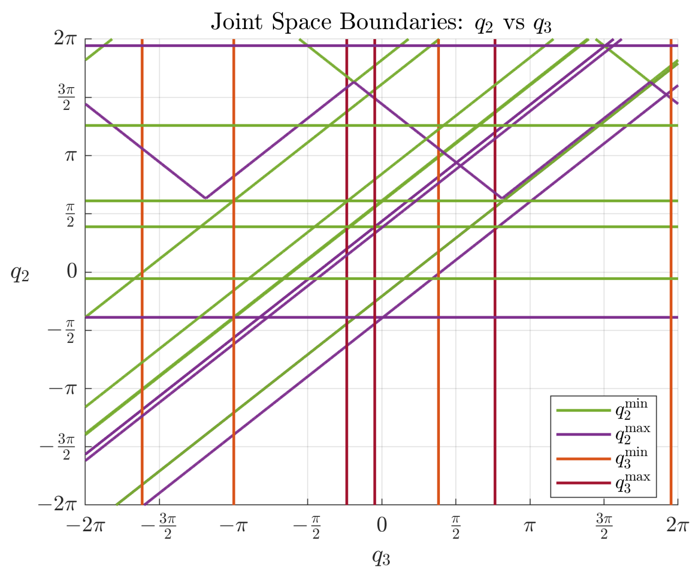
To visualize the feasible joint-space region defined by the symbolic boundary functions, a numerical evaluation was performed using the expressions presented in Equations (18)–(20). The resulting functions defining the lower and upper limits of q 2 as a function of q 3 , as well as the direct bounds on q 3 , were evaluated over a dense grid of joint configurations.
Figure 8 shows the corresponding boundary curves plotted in the q 2 vs. q 3 space. This graphical representation reveals the nonlinear and non-convex structure of the feasible region, emphasizing the importance of using analytical boundary models rather than simplified geometric approximations.
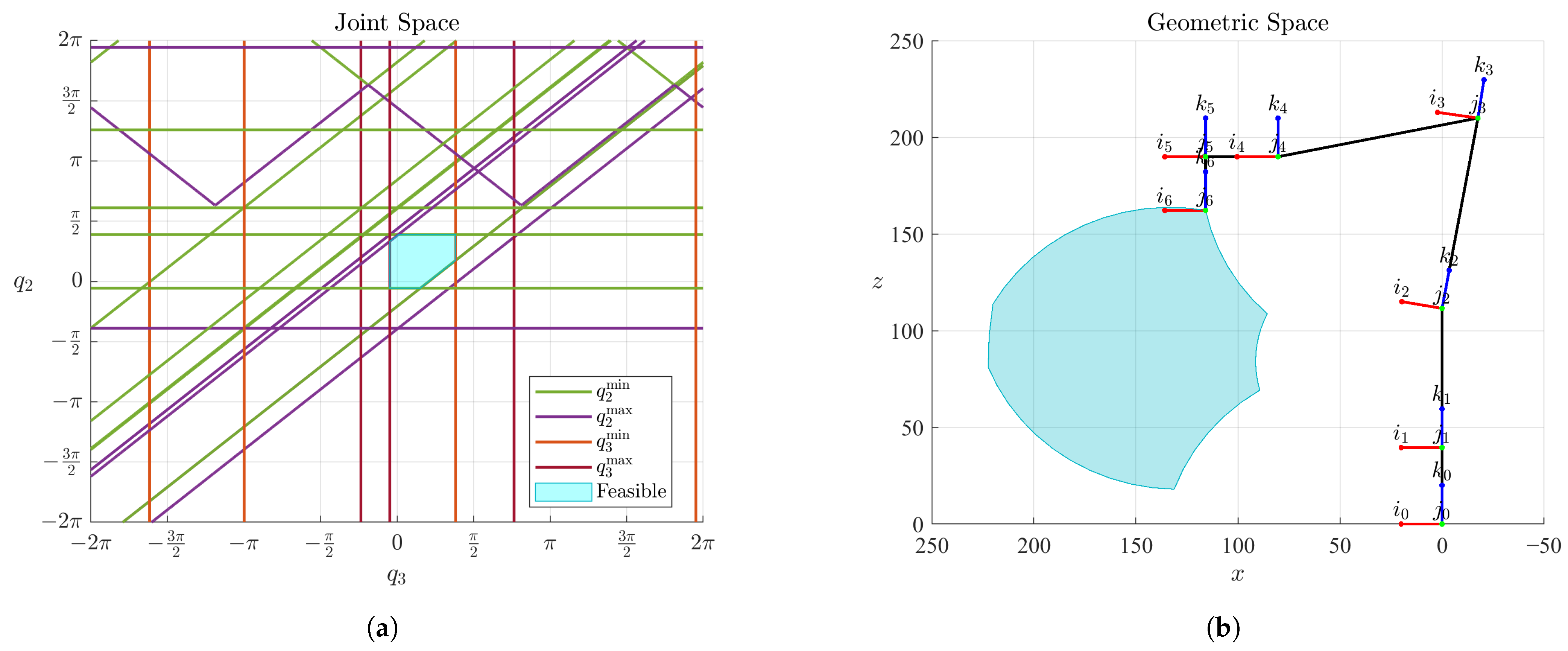
To extract the valid joint configurations from the overlapping boundary regions, a closed contour was constructed by interpolating between the intersection points of the active boundary functions. The resulting feasible region in joint space is shown in Figure 9, where the left panel illustrates the continuous shaded area of valid configurations. The right panel depicts the forward-mapped geometric workspace, derived from the direct kinematic evaluation of each point along the joint-space trajectory. This representation corresponds to the principal kinematic chain of the robot.

3.3. Scaling of Feasible Regions and Geometric Workspace Construction

To ensure a safety margin in trajectory planning, the originally constructed feasible region in joint space was uniformly scaled with respect to its centroid. This operation prevents configurations that lie exactly on the boundary functions, which are associated with potential collisions.
The original and scaled feasible regions in joint space were constructed by computing the intersection points of selected boundary functions, followed by a centroid-based scaling transformation to introduce a safety margin. These regions are shown in Figure 10, which also illustrates the corresponding geometric trajectories obtained through direct kinematic mapping.
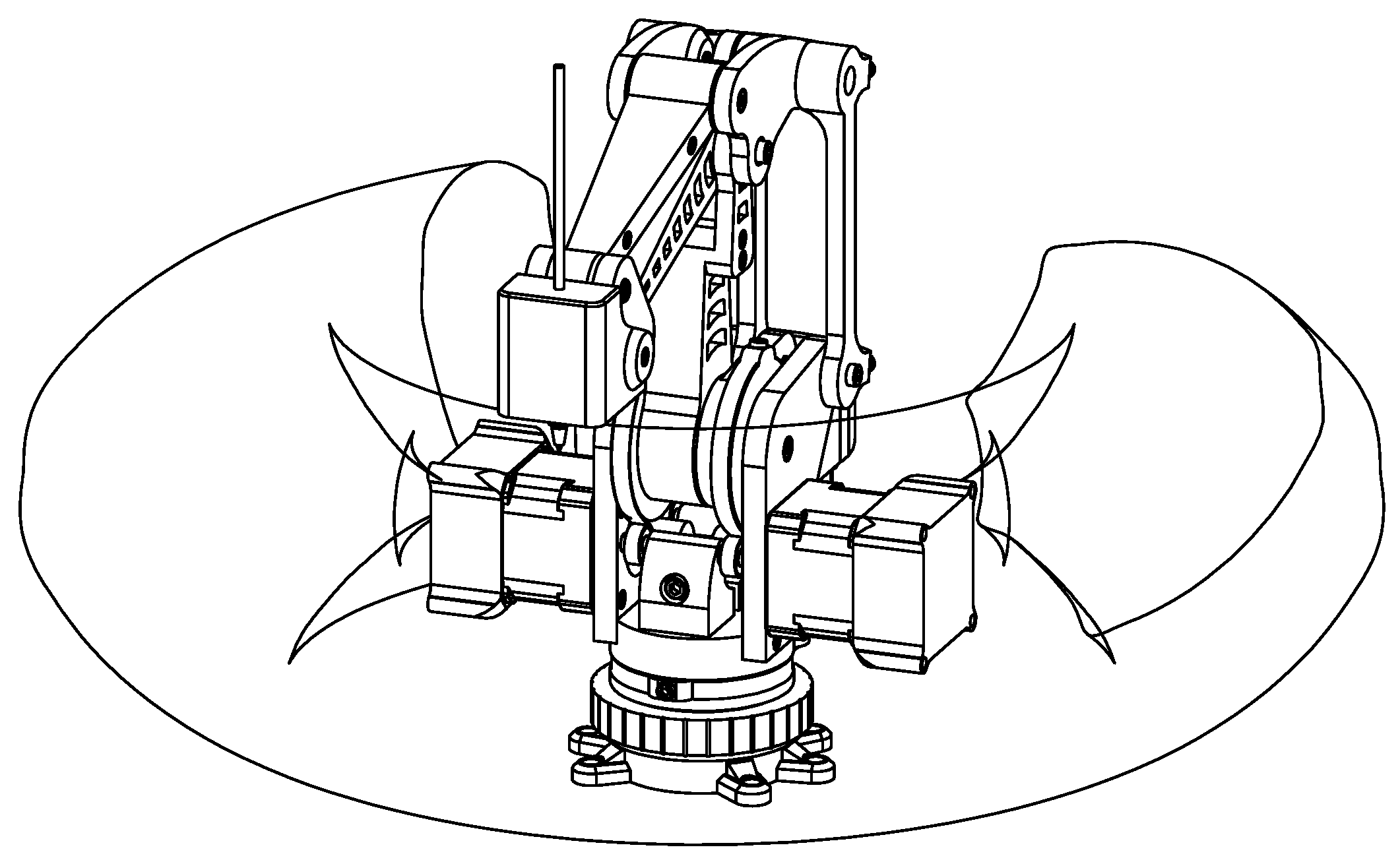
The complete volumetric feasible workspace was reconstructed by rotating the scaled joint-space trajectory about the base axis q 1 using discrete angular increments. This procedure leverages the inherent rotational symmetry of the manipulator to generate a continuous three-dimensional region that encompasses all reachable configurations free from internal collisions, as shown in Figure 11. A complementary CAD-based rendering of the resulting swept volume is presented in Figure 12, illustrating the workspace in the spatial frame of the robot.

3.4. Boundary Function Norms Along Original and Scaled Trajectories

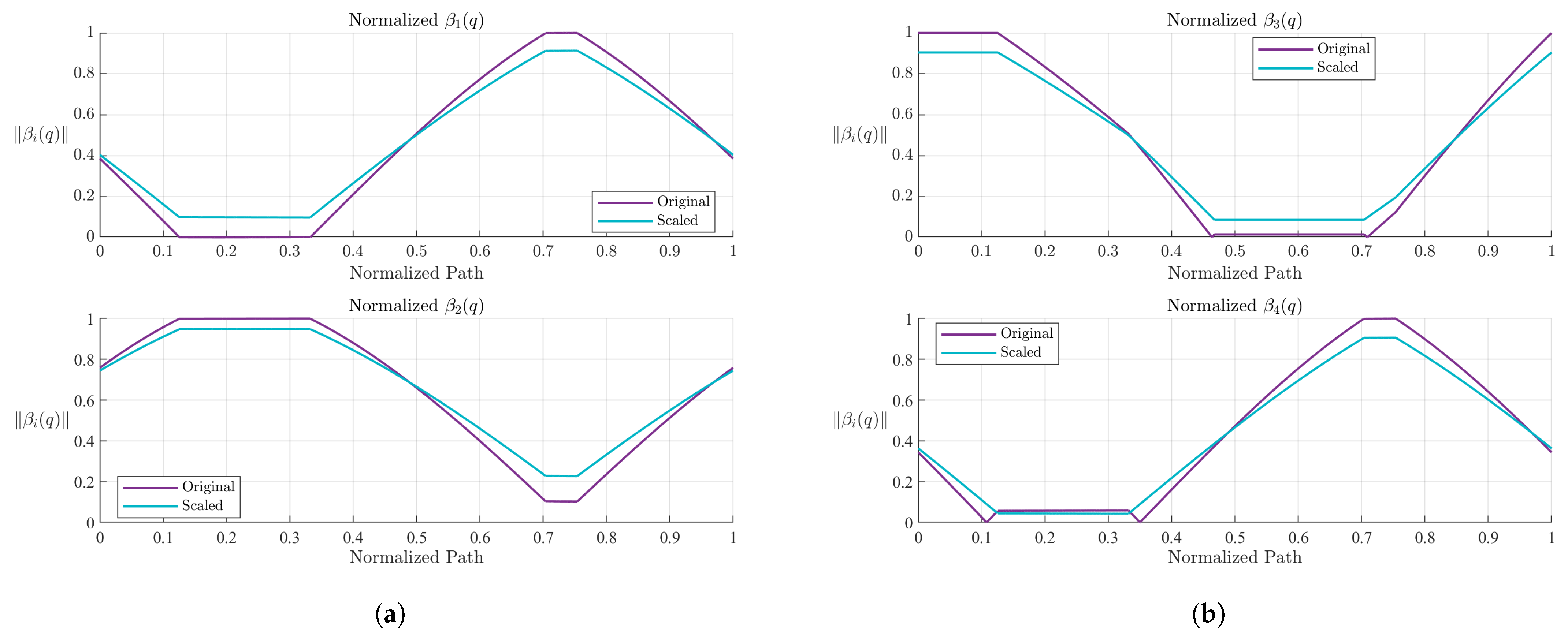
To further evaluate the effectiveness of the centroid-based scaling process, the norms of each boundary function β i ( q ) were computed along both the original and the scaled joint-space trajectories. These norms quantify the distance between each configuration and the corresponding constraint surface, allowing the detection of near-boundary conditions.
Figure 13 presents the results for the first four boundary functions. In the left subfigure, corresponding to β 1 ( q ) and β 2 ( q ) , it can be observed that the scaled trajectory increases the minimum norm in critical intervals, particularly where the original trajectory approaches near-zero values. Similarly, the right subfigure shows the behavior of β 3 ( q ) and β 4 ( q ) , where the scaled path systematically maintains greater distances from constraint boundaries, especially in the vicinity of sharp norm transitions.
In Figure 14, the next group of functions is analyzed. The left subfigure displays β 5 ( q ) and β 6 ( q ) , where the norm values along the scaled trajectory avoid deep local minima that occur in the original path. The right subfigure corresponds to β 7 ( q ) and β 8 ( q ) , showing similar benefits. The scaled version produces smoother transitions and consistently higher clearance margins across the normalized trajectory.
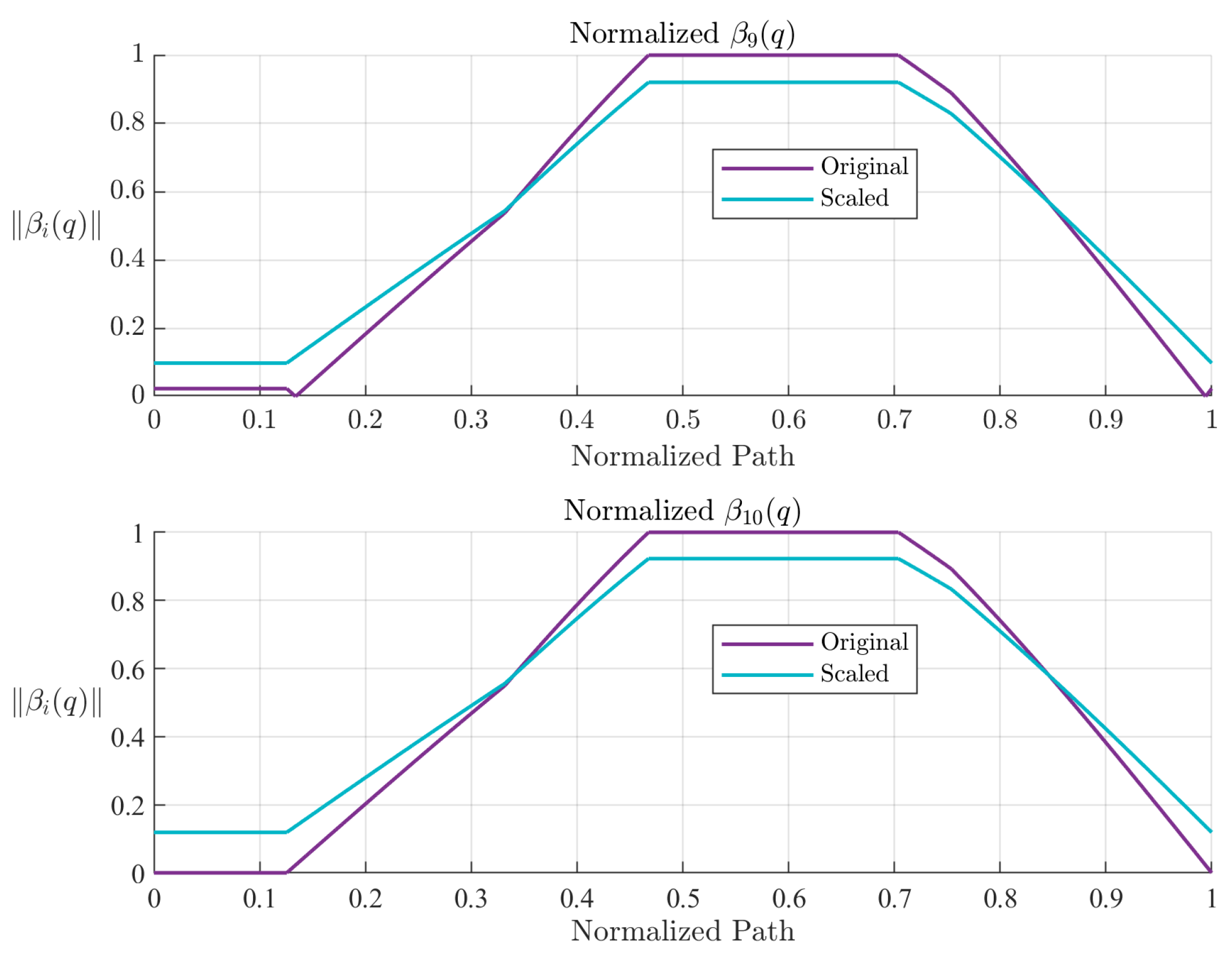
Figure 15 illustrates the final pair, β 9 ( q ) and β 10 ( q ) . The scaled trajectory not only increases the minimum values of the norm across the normalized path but also reduces the amplitude of variations, leading to a more consistent safety margin during execution.
These results confirm that the centroid-based transformation improves the clearance of all evaluated constraints, reducing the risk of boundary violations and enhancing the robustness of the robot’s feasible motion.

3.5. Dense Evaluation of Constraint Accumulation in Joint Space

To further validate the delineation of the feasible region, a dense sampling of the joint space was conducted. A total of 90,000 random configurations q = [ q 2 , q 3 ] [ 2 π , 2 π ] 2 were generated and evaluated against all boundary functions β i ( q ) . Each function’s absolute output was normalized and accumulated to quantify the overall constraint load at each configuration.
Additionally, each point was tested for inclusion within the polygonal feasible region using a containment test. The results were interpolated over a regular mesh to produce a scalar field representing the summed constraint activity across the joint space.
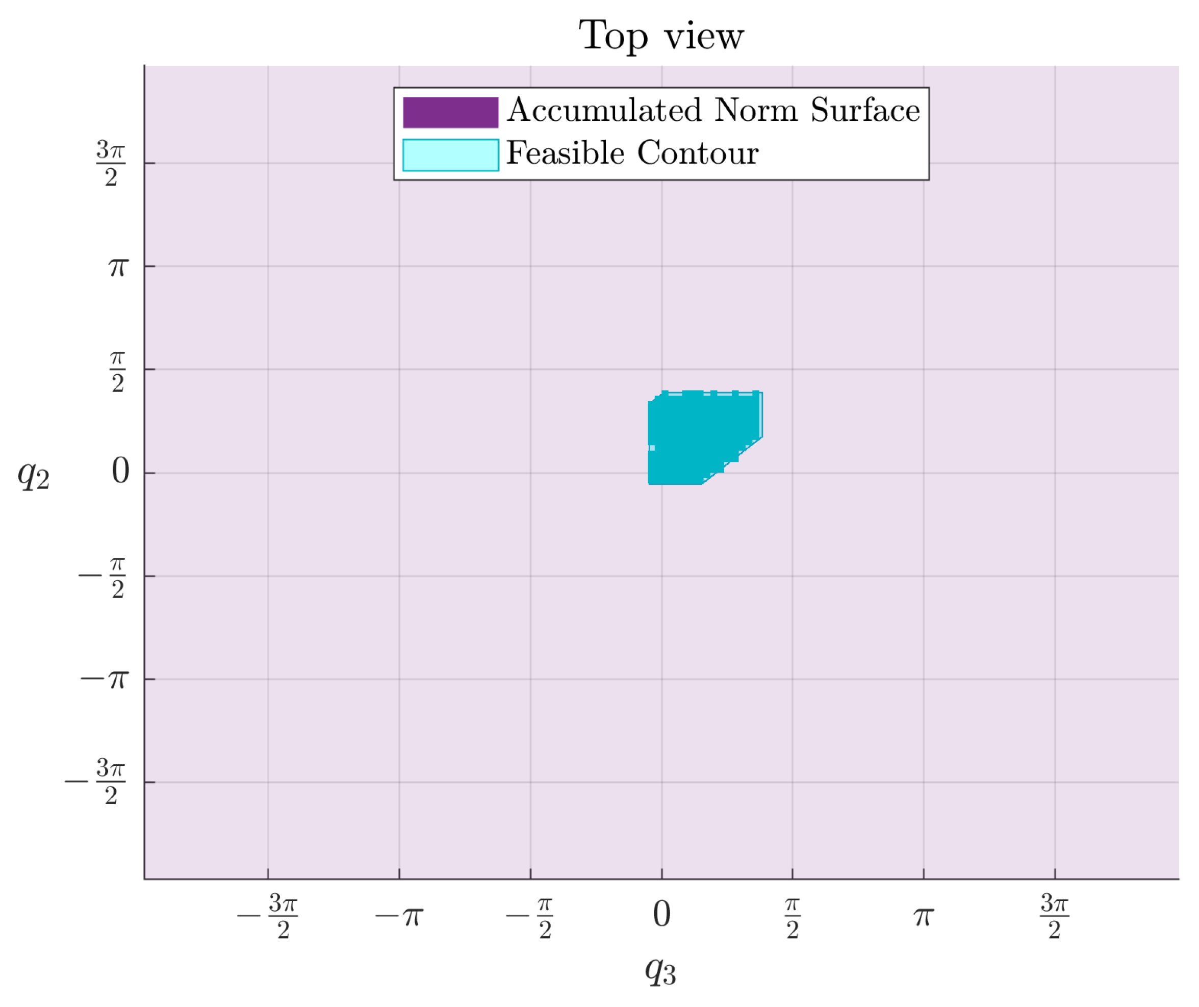
Figure 16 presents the resulting surface colored by feasibility classification. Regions inside the feasible contour are shown in turquoise, while external regions are marked in purple. The surface height encodes the total accumulated norm i β i ( q ) , highlighting the boundary layer surrounding the valid region.
To reinforce the spatial relationship, a top-down projection of the same surface is shown in Figure 17. This view confirms the sharp constraint gradient surrounding the feasible domain, and the regularity of the internal region defined by the symbolic formulation.

3.6. Numerical Validation with a Constructed Trajectory

To illustrate the practical application of the symbolic boundary framework, a numerical validation was performed using a proposed trajectory designed to traverse different levels of feasibility. This trajectory, originally defined in the geometric space and subsequently mapped to the joint space via inverse kinematics, was intentionally configured to include configurations both inside and outside the analytically defined feasible region.
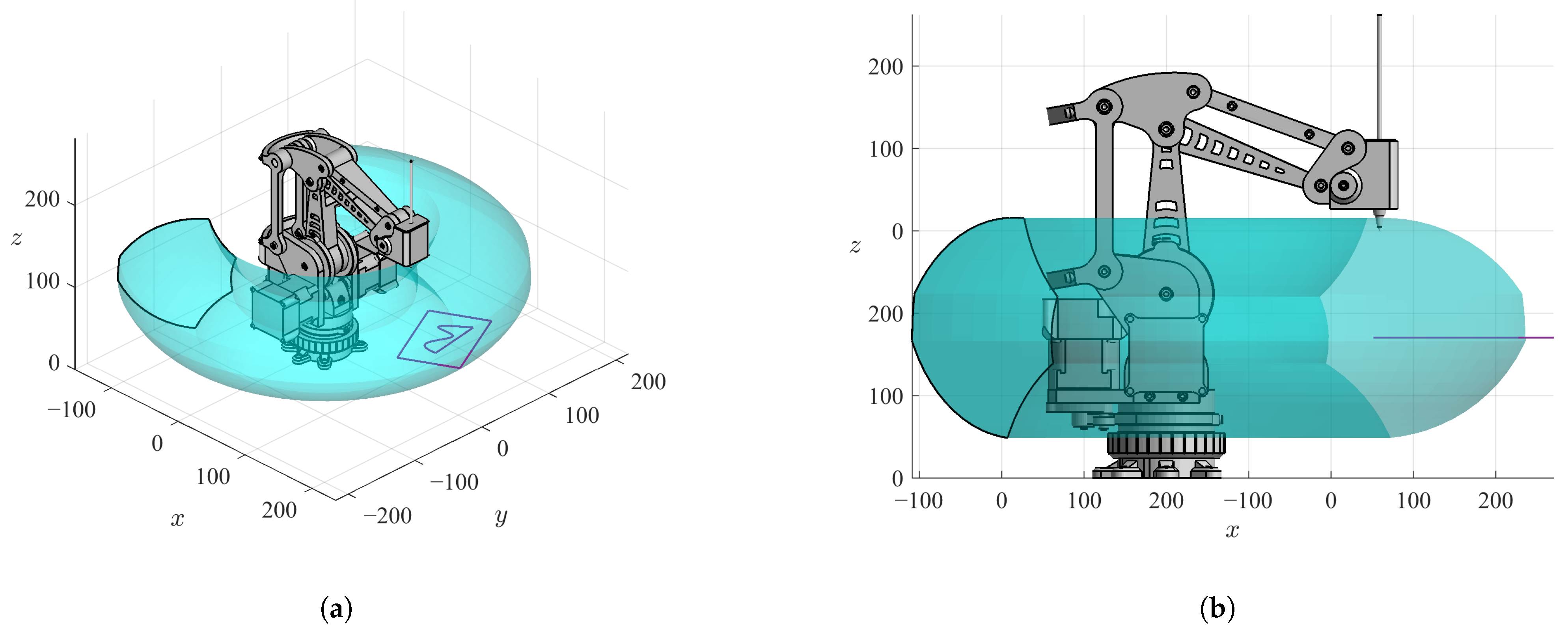
The geometric path was scaled and placed within the robot’s reachable volume, then evaluated using the direct and inverse kinematics of the MinervaBotV3. Figure 18a through Figure 19b show the spatial configuration of the robot along the trajectory, as well as multiple views of the feasible workspace and the proposed motion envelope.
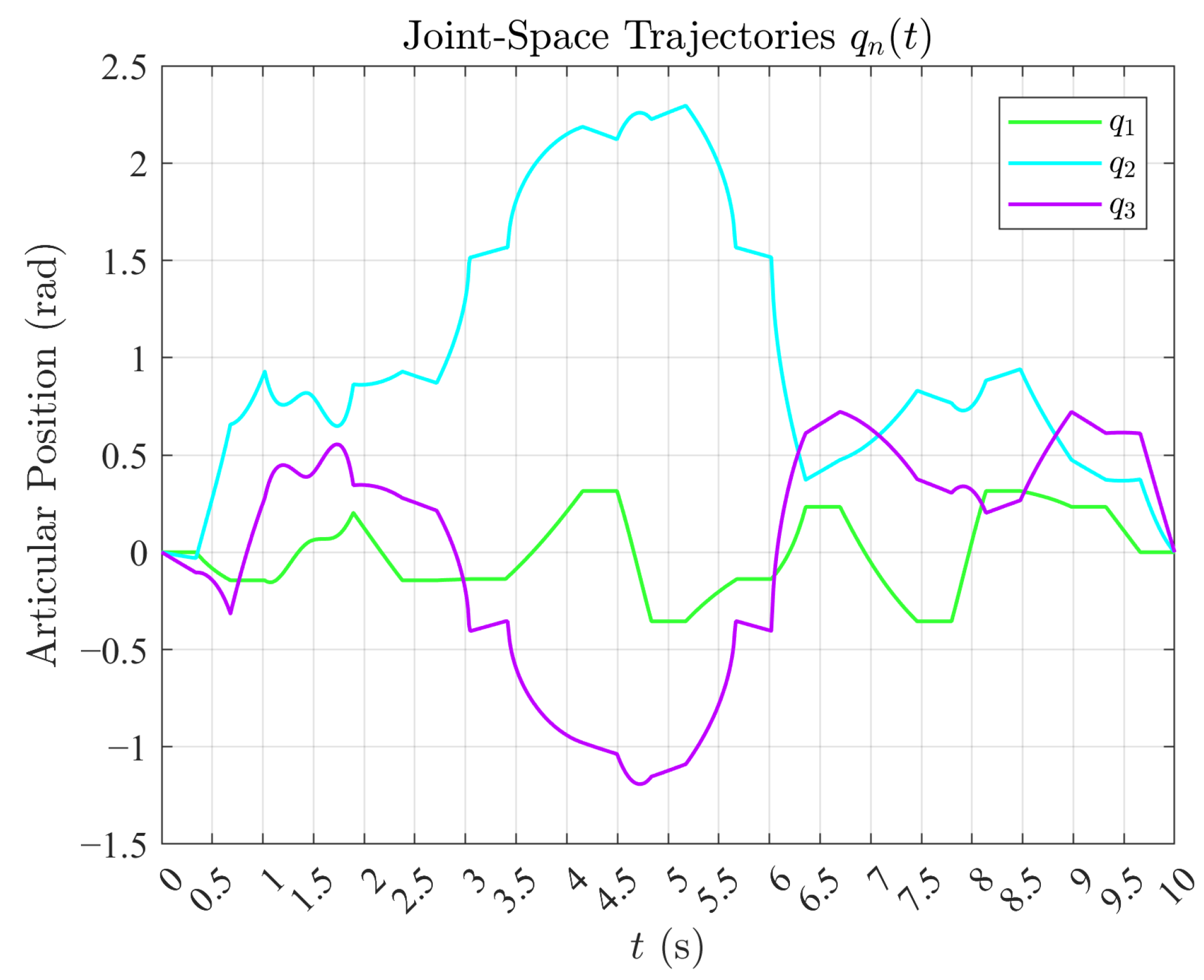
The joint trajectory q ( t ) = [ q 1 ( t ) , q 2 ( t ) , q 3 ( t ) ] was then extracted from the geometric path and analyzed symbolically (see Figure 20). The goal was not to optimize motion or control but to evaluate the behavior of the symbolic boundary functions when applied to realistic and diverse motion patterns.
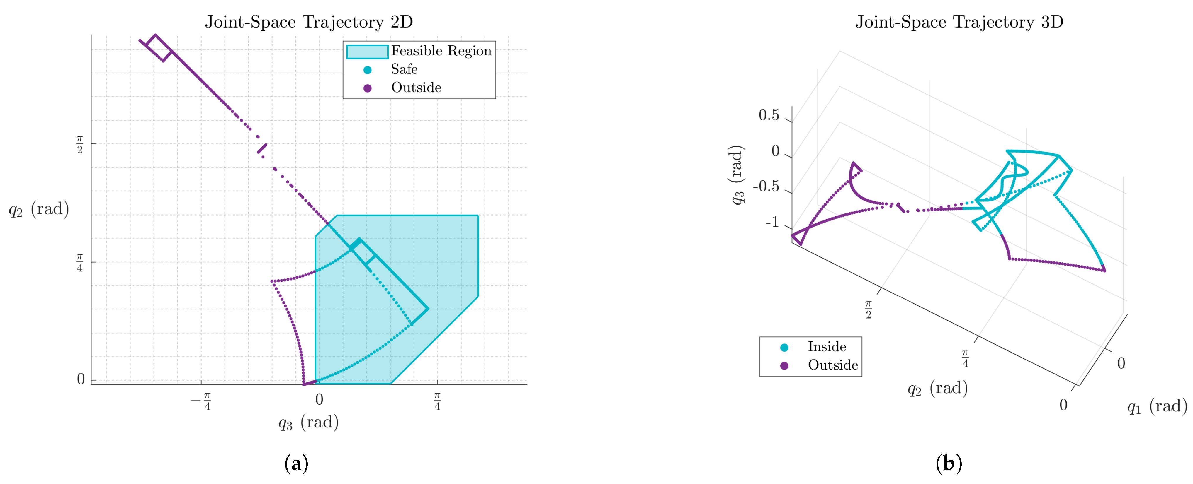
To assess the trajectory’s compliance with the joint-space limits, a symbolic classification was performed by projecting the joint positions onto the compressed boundary envelope. The polygonal region in the [ q 2 , q 3 ] plane was derived from the original collision contour using centroidal scaling, and joint positions were labeled based on whether they lie inside, on the boundary, or outside this region.
A full three-dimensional visualization of the joint trajectory within the compressed prism is provided in Figure 21b, confirming that the symbolic boundary framework successfully classifies each configuration without relying on numerical sampling or resolution heuristics.
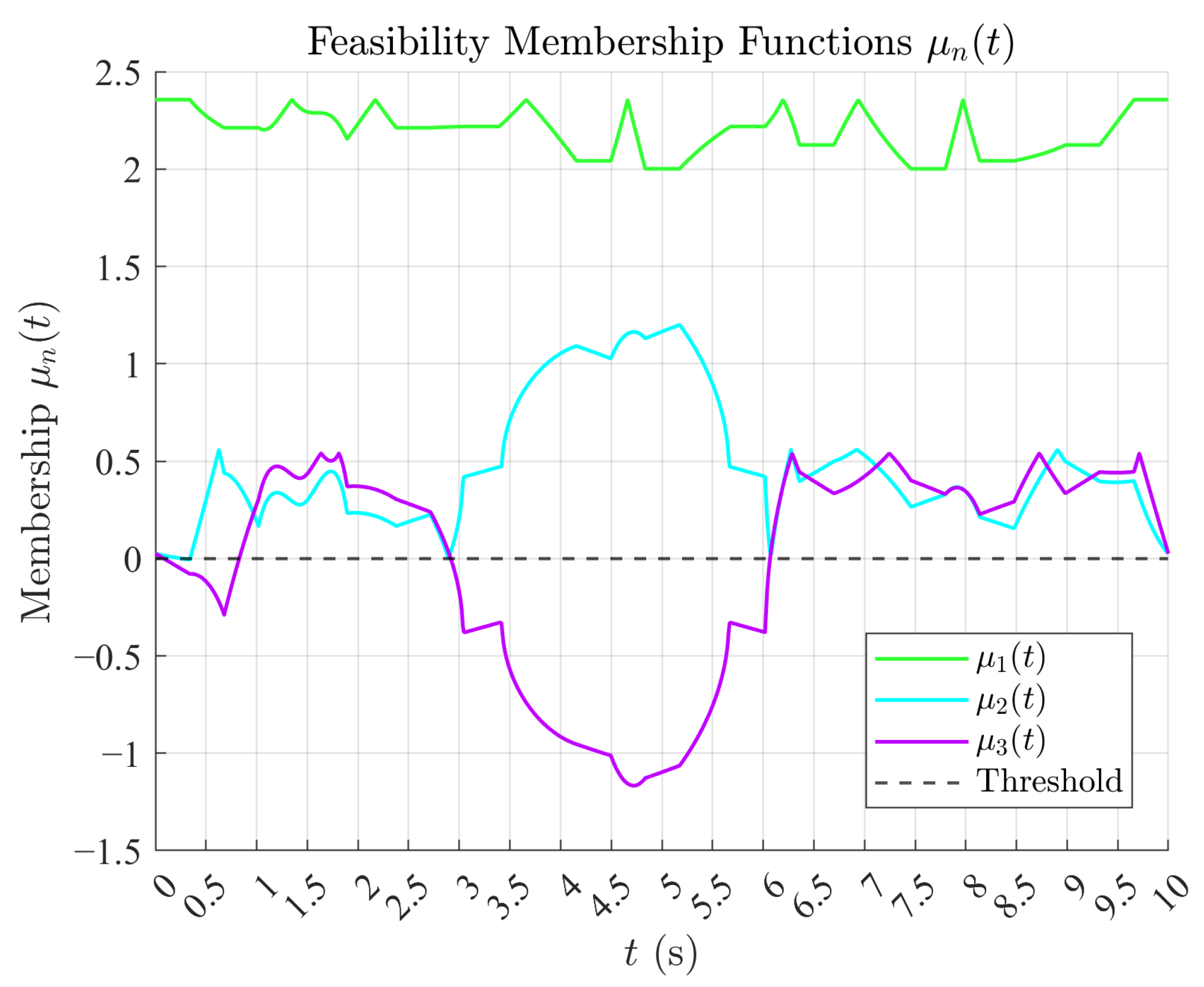
To better understand how symbolic boundary functions respond to real trajectories, a membership analysis was performed. The goal was to evaluate the degree to which each joint variable remains within its analytically defined safe region during the execution of the proposed trajectory.
For each joint variable q n ( t ) , a symbolic membership function μ n ( t ) was defined to quantify its relative position with respect to the feasible region delimited by analytical boundary functions. These functions are constructed to encode not only binary feasibility but also a continuous measure of clearance or violation, making them suitable for robustness analysis.
The sign and magnitude of μ n ( t ) carry semantic and quantitative meaning:
  • μ n ( t ) > 0 indicates that q n ( t ) lies strictly inside its feasible range, with the magnitude expressing the minimum distance to the nearest boundary.
  • μ n ( t ) = 0 represents contact with a constraint surface.
  • μ n ( t ) < 0 reflects violation of the feasibility condition, with the magnitude proportional to the depth of the intrusion.
Formally, for a joint variable q n ( t ) bounded between known analytical limits q n min and q n max , the membership function is defined as:
μ n ( t ) = q n ( t ) q n min , if q n ( t ) < q n min , min q n ( t ) q n min , q n max q n ( t ) , if q n min q n ( t ) q n max , q n ( t ) q n max , if q n ( t ) > q n max .
This piecewise definition guarantees that μ n ( t ) is continuous and differentiable within the interior of the feasible interval, while still conveying violation or contact at the boundaries.
In this work:
  • μ 1 ( t ) was evaluated directly from the physical joint limits of q 1 , as given by Equation (21). These limits were arbitrarily defined for illustrative purposes as [ 3 π 4 , 3 π 4 ] .
  • μ 2 ( t ) and μ 3 ( t ) were extracted from the scaled polygonal region in the [ q 2 , q 3 ] plane, which captures internal collision boundaries. Although the complete 2D polygon defines a joint constraint, each component was projected independently along q 2 and q 3 , and Equation (21) was applied along each axis using the corresponding minimum and maximum from the polygonal projection.
This formulation allows μ n ( t ) to serve as a feasibility metric that is both symbolic and numerically evaluable. Figure 22 shows the evolution of these functions for the proposed trajectory. This visualization not only determines whether the configuration is feasible at each time step but also provides a scalar metric to assess the robustness of each joint with respect to its active constraints.

3.7. Discussion of Symbolic Workspace Modeling

The formulation of boundary functions presented in this study offers a symbolic and interpretable approach for identifying collision-free configurations in planar manipulators with parallelogram mechanisms. Unlike sampling-based or ray-tracing methods, which often yield scattered or discontinuous feasible regions, the proposed method defines joint-space limits through closed-form analytical expressions derived from geometric constraints. This symbolic construction enables deeper theoretical insights into trajectory analysis, constraint interaction, and feasibility margins.
One of the principal strengths of this framework is its modularity: each boundary function encapsulates the interaction between a specific pair of structural elements. This localized encoding facilitates the debugging of the constraint, supports the integration of additional geometric conditions, and allows the selective activation of boundaries in reconfigurable or modular robot architectures.
The use of centroid-based scaling introduces effective operational safety margins by uniformly compressing the feasible region. This not only mitigates the risk of constraint violations due to model uncertainties, actuation errors, or discretization artifacts but also leads to more robust joint-space trajectories, as confirmed by the analysis of boundary function norms. The scaled regions maintain continuity and convexity properties, which are essential for reliable motion planning.
It is important to note that feasible joint trajectories do not necessarily map to smooth or symmetric operational paths. The nonlinearity of the forward kinematic map introduces geometric distortions in workspace shape, including asymmetries and curvature near the boundaries. This observation underscores the importance of analyzing feasibility not only in joint space but also in operational space, particularly for applications requiring precise end-effector placement or obstacle avoidance.
The symbolic framework developed here contrasts sharply with conventional sampling-based strategies such as those found in [9,15,21,22], and more recent data-driven methods based on neural networks [23]. While these approaches rely on discretized approximations or trained models to infer feasible regions, the symbolic boundary method directly encodes feasibility as an exact mathematical condition. Consequently, comparisons based on resolution, sampling density, or coverage metrics become unnecessary and conceptually redundant.
Although the current implementation targets planar mechanisms with three degrees of freedom, the symbolic methodology is extensible to spatial manipulators. However, the algebraic complexity of the resulting functions and their inverses increases significantly in higher dimensions. To address this, a symbolic-assisted algorithm based on root isolation and monotonic interval propagation is under development. This tool aims to enable efficient reconstruction and exploration of feasible joint-space regions in high-dimensional settings.
In summary, the integration of symbolic boundary functions, analytical inversion, and geometric scaling yields a structured modeling framework that is both mathematically rigorous and computationally tractable. Its inherent interpretability makes it well-suited not only for off-line analysis and planning but also for embedded robotic systems where transparency and safety guarantees are essential.

4. Conclusions

This study introduced a symbolic framework for the analytical definition of feasible workspaces in manipulator robots with parallelogram mechanisms. Unlike conventional sampling-based methods, the proposed approach constructs boundary functions derived from geometric and kinematic relationships between internal structural elements. These boundary functions define closed-form regions of feasible joint configurations, which are subsequently refined through centroid-based scaling to introduce safety margins and avoid singular configurations.
The methodology was applied to the MinervaBotV3 robot, whose planar geometry enabled the symbolic formulation of joint boundaries and corresponding geometric regions. The analysis revealed that the feasible workspace is continuous but asymmetric, and that the final pose of the robot is strongly influenced by the traversal sequence through the joint boundary. These results highlight the nonlinear nature of self-collision constraints and the advantages of explicit function modeling for workspace definition.
Furthermore, the analytical formulation facilitates the generation of structured, collision-free trajectories and enhances interpretability in both theoretical analysis and trajectory planning. This symbolic approach offers a scalable alternative to numerical methods by avoiding exhaustive sampling and enabling direct evaluation of constraint satisfaction.
Future work will address several extensions. First, the framework will be generalized to handle increased joint complexity and higher degrees of freedom, including redundant and over-actuated systems. Second, the symbolic formulation will be extended to spatial manipulators and hybrid kinematic chains, where boundary functions define implicit hypersurfaces in high-dimensional configuration spaces. Finally, the development of a dedicated algorithm for evaluating and traversing boundary functions—based on root-finding techniques, continuity constraints, and symbolic differentiation—is proposed to systematically construct feasible motion trajectories and support integration into planning architectures.

Author Contributions

Conceptualization, J.A.L. and L.F.L.-V.; methodology, J.A.L., H.A.G.-O. and J.R.N.; software, J.A.L., J.R.N. and D.M.N.; validation, L.F.L.-V., R.C.-N. and E.L.-N.; formal analysis, R.C.-N. and J.A.N.-P.; investigation, D.M.N. and J.R.N.; resources, L.F.L.-V. and J.A.N.-P.; data curation, E.L.-N., J.A.N.-P. and F.G.-V.; writing—original draft preparation, J.A.L. and D.M.N.; writing—review and editing, L.F.L.-V., H.A.G.-O. and R.C.-N.; visualization, E.L.-N. and F.G.-V.; supervision, J.A.L. and F.G.-V.; project administration, H.A.G.-O. and J.R.N.; funding acquisition, L.F.L.-V. and H.A.G.-O. All authors have read and agreed to the published version of the manuscript.

Funding

This research received no external funding.

Data Availability Statement

The data presented in this study are available on request from the corresponding author.

Acknowledgments

The authors thank the support of CINVESTAV and the Secretariat of Science, Humanities, Technology, and Innovation SECIHTI.

Conflicts of Interest

The authors declare no conflicts of interest.

References

  1. Siciliano, B.; Khatib, O. (Eds.) Springer Handbook of Robotics, 2nd ed.; Springer: Cham, Switzerland, 2016. [Google Scholar] [CrossRef]
  2. Gosselin, C.M.; Jean, M. Determination of the workspace of planar parallel manipulators with joint limits. Robot. Auton. Syst. 1996, 17, 129–138. [Google Scholar] [CrossRef]
  3. Sisbot, E.A.; Marin-Urias, L.M.; Alami, R.; Simeon, T. A Human Aware Mobile Robot Motion Planners. IEEE Trans. Robot. 2007, 23, 874–883. [Google Scholar] [CrossRef]
  4. Porges, O.; Leidner, D.; Roa, M. Planning Fail-Safe Trajectories for Space Robotic Arms. Front. Robot. AI 2021, 8, 710021. [Google Scholar] [CrossRef] [PubMed]
  5. Lacevic, B.; Rocco, P. Towards a complete safe path planning for robotic manipulators. In Proceedings of the 2010 IEEE/RSJ International Conference on Intelligent Robots and Systems, Taipei, Taiwan, 18–22 October 2010; pp. 5366–5371. [Google Scholar] [CrossRef]
  6. Khatib, O. Real-time obstacle avoidance for manipulators and mobile robots. Int. J. Robot. Res. 1986, 5, 90–98. [Google Scholar] [CrossRef]
  7. Min, F.; Wang, G.; Liu, N. Collision Detection and Identification on Robot Manipulators Based on Vibration Analysis. Sensors 2019, 19, 1080. [Google Scholar] [CrossRef] [PubMed]
  8. Lacevic, B.; Rocco, P. Kinetostatic danger field—A novel safety assessment for human-robot interaction. In Proceedings of the 2010 IEEE/RSJ International Conference on Intelligent Robots and Systems, Taipei, Taiwan, 18–22 October 2010; pp. 2169–2174. [Google Scholar] [CrossRef]
  9. Yang, X.; Wang, H.; Zhang, C.; Chen, K. A method for mapping the boundaries of collision-free reachable workspaces. Mech. Mach. Theory 2010, 45, 1024–1033. [Google Scholar] [CrossRef]
  10. Cao, J.; Tang, H.; Liu, X. Obstacle-free reachable workspace evaluation of industrial robots. Robot. Comput.-Integr. Manuf. 2017, 44, 240–252. [Google Scholar] [CrossRef]
  11. Cao, Y.; Guo, M.; Li, Y. Obstacle-free workspace based path planning for serial manipulator. In Proceedings of the 2017 36th Chinese Control Conference (CCC), Dalian, China, 26–28 July 2017; pp. 6897–6900. [Google Scholar] [CrossRef]
  12. Flacco, F.; Kroger, T.; Luca, A.D.; Khatib, O. Depth space safety for industrial robots. In Proceedings of the 2012 IEEE/RSJ International Conference on Intelligent Robots and Systems (IROS), Algarve, Portugal, October 7–12 2012; IEEE: New York, NY, USA, 2012; pp. 821–826. [Google Scholar] [CrossRef]
  13. Pham, D.T.; Afify, A.A. Machine learning techniques and their applications in manufacturing. Proc. Inst. Mech. Eng. Part B J. Eng. Manuf. 2005, 219, 395–412. [Google Scholar] [CrossRef]
  14. Qian, Y.; Yuan, J.; Wan, W. Improved Trajectory Planning Method for Space Robot-System with Collision Prediction. J. Intell. Robot. Syst. 2019, 99, 289–302. [Google Scholar] [CrossRef]
  15. Lacevic, B.; Osmankovic, D. Improved C-Space Exploration and Path Planning for Robotic Manipulators Using Distance Information. In Proceedings of the 2020 IEEE International Conference on Robotics and Automation (ICRA), Paris, France, 31 May–31 August 2020; pp. 1176–1182. [Google Scholar] [CrossRef]
  16. Mattila, J.; Koivumäki, J.; Caldwell, D.G.; Semini, C. A Survey on Control of Hydraulic Robotic Manipulators With Projection to Future Trends. IEEE/ASME Trans. Mechatron. 2017, 22, 669–680. [Google Scholar] [CrossRef]
  17. Sangiovanni, B.; Incremona, G.P.; Piastra, M.; Ferrara, A. Self-Configuring Robot Path Planning With Obstacle Avoidance via Deep Reinforcement Learning. IEEE Control Syst. Lett. 2021, 5, 397–402. [Google Scholar] [CrossRef]
  18. Singh, A.; Singla, A. Kinematic Modeling of Robotic Manipulators. Proc. Natl. Acad. Sci. India Sect. A Phys. Sci. 2017, 87, 303–319. [Google Scholar] [CrossRef]
  19. Chen, D.; Zhang, Y.; Li, S. Tracking Control of Robot Manipulators with Unknown Models: A Jacobian-Matrix-Adaption Method. IEEE Trans. Ind. Inform. 2018, 14, 3044–3053. [Google Scholar] [CrossRef]
  20. Lizarraga, J.A.; Navarro, D.M.; Mata-Romero, M.E.; Luque-Vega, L.F.; González-Jiménez, L.E.; Carrasco-Navarro, R.; Castro-Tapia, S.; Guerrero-Osuna, H.A.; López-Neri, E. Defining Feasible Joint and Geometric Workspaces Through Boundary Functions. Appl. Sci. 2025, 15, 5383. [Google Scholar] [CrossRef]
  21. Lara-Molina, F.A.; Dumur, D. Robust multi-objective optimization of parallel manipulators. Meccanica 2021, 56, 2773–2800. [Google Scholar] [CrossRef]
  22. Oetomo, D.; Daney, D.; Shirinzadeh, B.; Merlet, J.-P. An Interval-Based Method for Workspace Analysis of Planar Flexure-Jointed Mechanism. J. Mech. Des. 2008, 131, 011014. [Google Scholar] [CrossRef]
  23. Zhang, M.; Zhang, Z.; Ren, X. A Constrained Workspace Entrance Crossing Motion Generation Scheme Synthesized by Recurrent Neural Networks for Redundant Robot Manipulators. IEEE/ASME Trans. Mechatron. 2024; Early Access. [Google Scholar] [CrossRef]
Figure 1. General model for link boundary functions, where two arbitrary transformation paths converge at the global positions of points n and m. Their coincidence defines the collision condition.
Technologies 13 00404 g001
Figure 2. Kinematic chain with non-consecutive links and local points n and m, illustrating the recursive transformation propagation that leads to the boundary function expression.
Technologies 13 00404 g002
Figure 3. Kinematic chain with consecutive links and local points n and m, showing the recursive transformation propagation and the resulting boundary function expression.
Technologies 13 00404 g003
Figure 4. Kinematic chain with a bifurcation at frame a 1 = b 1 , leading to separate branches containing points n and m. The spatial relationship and resulting boundary function are illustrated.
Technologies 13 00404 g004
Figure 5. Kinematic chain with a symmetric bifurcation where r a 1 , a = r a 1 , b . The collision condition depends solely on the branches’ local orientations and internal geometry.
Technologies 13 00404 g005
Figure 6. MinervaBotV3 palletizing robot by Mythbots, scaled at 1:2 for educational applications.
Technologies 13 00404 g006
Figure 8. Joint-space limits defined by the lower and upper boundary functions for the angular variables q 2 and q 3 . The curves q 2 min ( q 3 ) , q 2 max ( q 3 ) , q 3 min ( q 2 ) , and q 3 max ( q 2 ) were numerically evaluated over a dense grid and plotted to visualize the feasible joint region. These boundary functions were previously constructed using the symbolic formulation of collision constraints.
Technologies 13 00404 g008
Figure 9. Feasible workspace construction from joint-space analysis. (a) Closed contour formed by interpolating intersection points of selected boundary functions, yielding the valid configuration region in joint space. (b) Corresponding geometric workspace obtained via direct kinematic mapping of the closed trajectory, representing the principal kinematic chain.
Technologies 13 00404 g009
Figure 10. Comparison between original and scaled trajectories. (a) Feasible joint-space regions before and after centroid-based scaling transformation. (b) Corresponding spatial trajectories, where the scaled region preserves a collision-free configuration throughout its motion.
Technologies 13 00404 g010
Figure 11. Swept volume generated by rotating the scaled joint-space boundary around axis q 1 , forming a continuous and symmetric volumetric region.
Technologies 13 00404 g011
Figure 12. CAD-based rendering of the MinervaBotV3 workspace, visualizing the spatial region that can be reached without self-collision.
Technologies 13 00404 g012
Figure 13. Norms of the first four boundary functions along the original and scaled trajectories. The scaled path increases distance to constraint surfaces, enhancing robustness. (a) β 1 ( q ) and β 2 ( q ) . (b) β 3 ( q ) and β 4 ( q ) .
Technologies 13 00404 g013
Figure 14. Norms for β 5 ( q ) through β 8 ( q ) along original and scaled trajectories, showing increased clearance from constraint boundaries due to scaling. (a) β 5 ( q ) and β 6 ( q ) . (b) β 7 ( q ) and β 8 ( q ) .
Technologies 13 00404 g014
Figure 15. Norms of the final pair of boundary functions. The scaled trajectory consistently maintains a safer distance from constraint surfaces.
Technologies 13 00404 g015
Figure 16. Accumulated norm surface over joint space. The surface height corresponds to the sum of normalized constraint functions i β i ( q ) . Transparent coloring distinguishes the feasible region (turquoise) from its surroundings (purple).
Technologies 13 00404 g016
Figure 17. Top-down view of the accumulated constraint surface. The polygonal feasible region is shown in cyan, surrounded by a gradient field representing increasing constraint activity.
Technologies 13 00404 g017
Figure 18. Geometric evaluation of the proposed trajectory: global spatial context. (a) Isometric view of the proposed trajectory within the feasible workspace of the robot. (b) Lateral view of the robot and the geometric path used for validation.
Technologies 13 00404 g018
Figure 19. Geometric evaluation of the proposed trajectory: local and detailed views. (a) Top-down view of the trajectory over the planar workspace of the robot. (b) Zoomed visualization of the scaled trajectory traced in the 3D workspace (bridges included).
Technologies 13 00404 g019
Figure 20. Time-varying joint positions along the proposed trajectory. The curves q 1 ( t ) , q 2 ( t ) , and q 3 ( t ) reveal the complexity and diversity of motion patterns included for symbolic evaluation (bridges included).
Technologies 13 00404 g020
Figure 21. Symbolic feasibility classification of the proposed trajectory. The 2D and 3D views confirm that the symbolic boundary functions successfully detect constraint violations. The joint limits for q 1 were arbitrarily set to ± 3 π 4 . (a) Symbolic classification of the joint trajectory in the [ q 2 , q 3 ] plane. (b) The 3D projection of the joint trajectory in ( q 1 , q 2 , q 3 ) space.
Technologies 13 00404 g021
Figure 22. Symbolic membership functions μ n ( t ) for each joint variable. Positive values indicate feasibility, zero denotes contact with the constraint, and negative values correspond to violations.
Technologies 13 00404 g022
Table 1. Robots.
Table 1. Robots.
No. SerieManufacturerParallelogramsRelevant Characteristics
KR 700PAKUKA2Total load: 700 kg, maximum reach: 3320 mm.
IRB 760ABB3Axes: 4, long reach, full-layer palletizer.
IRB 4400ABB1Robust construction, double bearing joints, optimized torque.
M-410iB/700FANUC2Controlled axes: 4, payload: 700 kg, reach: 3143 mm.
HP 160 OHYUNDAI2Payload: 160 kg, max reach: 3128 mm, high speed.
PAL-260-3.1COMAU1Axes: 4, max wrist payload: 260 kg.
PAL-180-3.1COMAU1Axes: 4, max wrist payload: 180 kg.
FD-LP130OTC2Axes: 4, type of robot: palletizing, capacity: 130 kg or 180 kg.
MC1000DLNACHI2Designed for lifting up to 1000 kg, superior strength, long reach.
SC700DLNACHI2Payload: 700 kg, axes: 6, robot mass: 7000 kg.
MC600NACHI1Heavy lifting: 600 kg, work envelope: 2890 mm.
FD-A20DAIHEN1Payload: 20 kg for laser welding torch, axes: 6, high accuracy.
TC1010B-140TANG CHENG2Payload: 10 kg, axes: 4, repeat precision: ±0.08 mm.
M-410iC/110FANUC2Controlled axes: 4, payload: 110 kg, reach: 2403 mm.
M-410iC/185FANUC1Controlled axes: 4, payload: 185 kg, reach: 3143 mm.
PL500YASKAWA1Axes: 4, robot category: palletizing.
RMD08GSK2Axes: 4, max payload: 8 kg, robot mass: 180 kg.
RMD20GSK2Axes: 4, max payload: 20 kg, robot mass: 256 kg.
RMD120GSK2Axes: 4, max payload: 120 kg, robot mass: 1500 kg.
CP180LKAWASAKI1Payload: 180 kg, max reach: 3255 mm, robot category: palletizing.
MPL160-100IIKAWASAKI2Axes: 4, payload: 100 kg, max working range: 3159 mm.
MPL160 IIKAWASAKI2Axes: 4, robot category: palletizing, vertical reach: 3024 mm, horizontal reach: 3159 mm.
ER60-2000-PLESTUN2Axes: 4, payload: 60 kg, reach: 2000 mm.
ER120-2400-PLESTUN2Axes: 4, payload: 120 kg, reach: 2400 mm.
SF15-C1538CHAIFU2Maximum radius: 53 mm, payload: 15 kg, repeatability: ± 0.08 mm.
SF8-K1400CHAIFU2Maximum radius: 1492 mm, payload: 8 kg, repeatability: ± 0.07 mm.
QJRB30-1QJAR2Axes: 4, payload: 30 kg, repeat positioning: ±0.05 mm.
QJRB800-1QJAR2Axes: 4, payload: 800 kg, repeat positioning: ±0.05 mm.
BRTIRPZ2250ABORUTE2Axes: 4, reach: 2200 mm, payload: 50 kg, high precision.
BRTIRPZ3013ABORUTE2Max load: 130 kg, reach: 3020 mm, designed for repetitive industrial tasks.
BRTIRPZ1508ABORUTE2Max load: 8 kg, max reach: 1500 mm.
JZJ10B-140JZJRT2Axes: 6, weight capacity: 20 kg, position repeatability: ±0.08 mm.
JZJ25B-180JZJRT2Axes: 4, reach: 1800 mm, payload capacity: 25 kg.
Table 2. Symbols used in the formulation of joint and link boundary functions.
SymbolDescription
q R n Vector of joint variables
q n ( t ) n-th joint variable as a function of time
μ n ( t ) Symbolic membership function for q n ( t )
W q Feasible region in joint space
W g Feasible geometric workspace in R 3
p = f ( q ) Geometric position mapped from joint configuration
β ( q ) Scalar boundary function
β i ( q ) i-th boundary function
r i , j Position vector from frame i to frame or point j
r a + n , b + m Relative vector between local points on links a and b
· Euclidean norm (vector magnitude)
R i , j Rotation matrix from frame j to frame i
R a , b = R a , c R c , b Recursive composition of orientation matrices
a + n Local point n rigidly attached to frame a
b + m Local point m rigidly attached to frame b
n, mPoint indices relative to their local frames
a, bFrames along a kinematic chain
a 1 , b 1 Common ancestor frame for branched topologies
0, 0 Global or alternative base frames
d min Minimum allowable distance to prevent collision
Table 3. Geometric offsets of MinervaBotV3.
ParameterSymbolValue (mm)
Offset z (Base to Joint 1) z 0 , 1 38.5
Offset z (Joint 1 to Joint 2) z 1 , 2 72
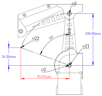
Offset z (Joint 2 to Joint 3) z 2 , 3 100
Offset x (Joint 3 to Joint 4) x 3 , 4 93.97
Offset z (Joint 3 to Joint 4) z 3 , 4 −34.20
Offset x (Joint 4 to Joint 5) x 4 , 5 35.46
Offset z (Joint 5 to End Effector) z 5 , 6 −27.71
Table 4. Recursive notation of the position vectors of the MinervaBotV3.
PointPosition VectorMatrixOrientation
r 0 , 1 0 0 z 0 , 1 T R 0 , 1 R z ( q 1 )
r 1 , 2 0 0 z 1 , 2 T R 1 , 2 R y ( q 2 )
r 2 , 3 0 0 z 2 , 3 T R 2 , 3 R y ( q 2 + q 3 )
r 3 , 4 x 3 , 4 0 z 3 , 4 T R 3 , 4 R y ( q 3 )
r 4 , 5 x 4 , 5 0 0 T R 4 , 5 R y ( 0 )
r 5 , 6 0 0 z 5 , 6 T R 5 , 6 I
r 0 , 2 r 0 , 1 + R 0 , 1 r 1 , 2 R 0 , 2 R 0 , 1 R 1 , 2
r 0 , 3 r 0 , 2 + R 0 , 2 r 2 , 3 R 0 , 3 R 0 , 2 R 2 , 3
r 0 , 4 r 0 , 3 + R 0 , 3 r 3 , 4 R 0 , 4 R 0 , 3 R 3 , 4
r 0 , 5 r 0 , 4 + R 0 , 4 r 4 , 5 R 0 , 5 R 0 , 4 R 4 , 5
r 0 , 6 r 0 , 5 + R 0 , 5 r 5 , 6 R 0 , 6 R 0 , 5 R 5 , 6
Table 5. Type: Consecutive Link Boundary Function β 1 ( q ) . This boundary function corresponds to a potential collision between two consecutive components. o 7 is defined in system o 2 , and o 8 in system o 3 . The scalar function β 1 ( q ) evaluates the Euclidean distance between their transformed representations in o 2 .
GraphicGeometric Offsets and Boundary Functions
Technologies 13 00404 i001
x 2 , 7 = 9.69 mm , z 2 , 7 = 68.27 mm
x 3 , 8 = 27.00 mm , z 3 , 8 = 19.27 mm
r 2 , 7 = x 2 , 7 0 z 2 , 7 , r 3 , 8 = x 3 , 8 0 z 3 , 8
β 1 ( q ) = r 2 , 7 r 2 , 3 R 2 , 3 r 3 , 8
β 1 ( q ) = 0 j { 1 , 2 , 3 } , β 1 , j = 0 |
β 1 , 1 β 1 , 2 β 1 , 3 = x 2 , 7 x 3 , 8 cos ( q 2 q 3 ) + z 3 , 8 sin ( q 2 q 3 ) 0 z 2 , 7 z 3 , 8 cos ( q 2 q 3 ) x 3 , 8 sin ( q 2 q 3 ) z 2 , 3 .
Table 6. Type: Consecutive Link Boundary Function β 2 ( q ) . This boundary function corresponds to a potential collision between two consecutive components. o 9 is defined in system o 2 , and o 10 in system o 3 . The scalar function β 2 ( q ) evaluates the Euclidean distance between their transformed representations in o 2 . A collision occurs if and only if β 2 ( q ) = 0 .
GraphicGeometric Offsets and Boundary Functions
Technologies 13 00404 i002
x 2 , 9 = 10.03 mm , z 2 , 9 = 64.85 mm
x 3 , 10 = 36.45 mm , z 3 , 10 = 2.74 mm
r 2 , 9 = x 2 , 9 0 z 2 , 9 , r 3 , 10 = x 3 , 10 0 z 3 , 10
β 2 ( q ) = r 2 , 9 r 2 , 3 R 2 , 3 r 3 , 10
β 2 ( q ) = 0 j { 1 , 2 , 3 } , β 2 , j = 0 |
β 2 , 1 β 2 , 2 β 2 , 3 = x 2 , 9 x 3 , 10 cos ( q 2 q 3 ) + z 3 , 10 sin ( q 2 q 3 ) 0 z 2 , 9 z 3 , 10 cos ( q 2 q 3 ) x 3 , 10 sin ( q 2 q 3 ) z 2 , 3 .
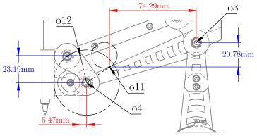
Table 7. Type: Consecutive Link Boundary Function β 3 ( q ) . This boundary function corresponds to a potential collision between two consecutive components. o 11 is defined in system o 3 , and o 12 in system o 4 . The scalar function β 3 ( q ) evaluates the Euclidean distance between their transformed representations in o 3 . A collision occurs if and only if β 3 ( q ) = 0 .
GraphicGeometric Offsets and Boundary Functions
  Technologies 13 00404 i003
x 3 , 11 = 74.29 mm , z 3 , 11 = 20.78 mm
x 4 , 12 = 5.47 mm , z 4 , 12 = 23.19 mm
r 3 , 11 = x 3 , 11 0 z 3 , 11 , r 4 , 12 = x 4 , 12 0 z 4 , 12
β 3 ( q ) = r 3 , 11 r 3 , 4 R 3 , 4 r 4 , 12
β 3 ( q ) = 0 j { 1 , 2 , 3 } , β 3 , j = 0 |
β 3 , 1 β 3 , 2 β 3 , 3 = x 3 , 11 x 3 , 4 x 4 , 12 cos ( q 3 ) + z 4 , 12 sin ( q 3 ) 0 z 3 , 11 z 3 , 4 z 4 , 12 cos ( q 3 ) x 4 , 12 sin ( q 3 ) .
Table 8. Type: Coincident Branched Link Boundary Function β 4 ( q ) . This function models a potential collision between two components attached to separate branches. o 14 and o 15 belong to distinct kinematic chains and are both expressed with respect to the common reference system o 1 . The scalar function β 4 ( q ) measures their distance in that shared frame. A collision occurs when β 4 ( q ) = 0 .
GraphicGeometric Offsets and Boundary Functions
Technologies 13 00404 i004
x 2 , 14 = 13.44 mm , z 2 , 14 = 30.61 mm
x 13 , 15 = 27.76 mm , z 13 , 15 = 18.63 mm
r 2 , 14 = x 2 , 14 0 z 2 , 14 , r 13 , 15 = x 13 , 15 0 z 13 , 15
R 1 , 2 = R y ( q 2 ) , R 1 , 13 = R y ( q 3 )
β 4 ( q ) = R 1 , 2 r 2 , 14 R 1 , 13 r 13 , 15
β 4 ( q ) = 0 j { 1 , 2 , 3 } , β 4 , j = 0 |
β 4 , 1 β 4 , 2 β 4 , 3 = x 2 , 14 cos ( q 2 ) x 13 , 15 cos ( q 3 ) z 13 , 15 sin ( q 3 ) + z 2 , 14 sin ( q 2 ) 0 z 2 , 14 cos ( q 2 ) z 13 , 15 cos ( q 3 ) + x 13 , 15 sin ( q 3 ) x 2 , 14 sin ( q 2 ) .
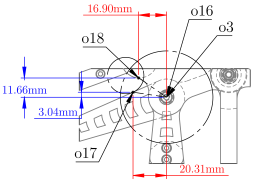
Table 9. Type: Coincident Branched Link Boundary Function β 5 ( q ) . This function models a potential collision between two components attached to separate branches originating from a common ancestor. o 17 and o 18 belong to distinct branches and are both expressed with respect to the shared reference system o 2 . The scalar function β 5 ( q ) evaluates the distance between them. A collision is detected when β 5 ( q ) = 0 .
GraphicGeometric Offsets and Boundary Functions
Technologies 13 00404 i005
x 3 , 17 = 20.31 mm , z 3 , 17 = 3.04 mm
x 16 , 18 = 16.90 mm , z 16 , 18 = 11.66 mm
r 3 , 17 = x 3 , 17 0 z 3 , 17 , r 16 , 18 = x 16 , 18 0 z 16 , 18
R 2 , 3 = R y ( q 2 + q 3 ) , R 2 , 16 = R y ( q 3 )
β 5 ( q ) = R 2 , 3 r 3 , 17 R 2 , 16 r 16 , 18
β 5 ( q ) = 0 j { 1 , 2 , 3 } , β 5 , j = 0 |
β 5 , 1 β 5 , 2 β 5 , 3 = x 3 , 17 cos ( q 2 q 3 ) z 16 , 18 sin ( q 3 ) x 16 , 18 cos ( q 3 ) z 3 , 17 sin ( q 2 q 3 ) 0 x 16 , 18 sin ( q 3 ) z 16 , 18 cos ( q 3 ) + z 3 , 17 cos ( q 2 q 3 ) + x 3 , 17 sin ( q 2 q 3 ) .
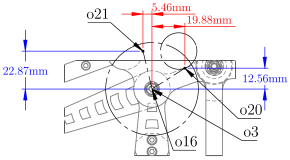
Table 10. Type: Coincident Branched Link Boundary Function β 6 ( q ) . This function represents a potential collision between two components belonging to distinct kinematic branches. o 20 and o 21 are defined in different branches and are transformed into the shared reference system o 2 . The scalar function β 6 ( q ) evaluates the distance between them. A collision is detected when β 6 ( q ) = 0 .
GraphicGeometric Offsets and Boundary Functions
Technologies 13 00404 i006
x 3 , 20 = 19.88 mm , z 3 , 20 = 12.56 mm
x 16 , 21 = 5.46 mm , z 16 , 21 = 22.87 mm
r 3 , 20 = x 3 , 20 0 z 3 , 20 , r 16 , 21 = x 16 , 21 0 z 16 , 21
R 2 , 3 = R y ( q 2 + q 3 ) , R 2 , 16 = R y ( q 3 )
β 6 ( q ) = R 2 , 3 r 3 , 20 R 2 , 16 r 16 , 21
β 6 ( q ) = 0 j { 1 , 2 , 3 } , β 6 , j = 0 |
β 6 , 1 β 6 , 2 β 6 , 3 = x 3 , 20 cos ( q 2 q 3 ) z 16 , 21 sin ( q 3 ) x 16 , 21 cos ( q 3 ) z 3 , 20 sin ( q 2 q 3 ) 0 x 16 , 21 sin ( q 3 ) z 16 , 21 cos ( q 3 ) + z 3 , 20 cos ( q 2 q 3 ) + x 3 , 20 sin ( q 2 q 3 ) .
Table 11. Type: Coincident Branched Link Boundary Function β 7 ( q ) . This function models a potential collision between two components belonging to different branches of the kinematic structure. o 3 is defined in system o 2 , and o 22 in system o 21 . Both are transformed into the common reference frame o 1 , and the scalar function β 7 ( q ) evaluates the distance between them. A collision occurs when β 7 ( q ) = 0 .
GraphicGeometric Offsets and Boundary Functions
Technologies 13 00404 i007
x 2 , 3 = 0 mm , z 2 , 3 = 100.00 mm
x 21 , 22 = 93.97 mm , z 21 , 22 = 34.20 mm
r 2 , 3 = x 2 , 3 0 z 2 , 3 , r 21 , 22 = x 21 , 22 0 z 21 , 22
R 1 , 2 = R y ( q 2 ) , R 1 , 21 = I
β 7 ( q ) = R 1 , 2 r 2 , 3 R 1 , 21 r 21 , 22
β 7 ( q ) = 0 j { 1 , 2 , 3 } , β 7 , j = 0 |
β 7 , 1 β 7 , 2 β 7 , 3 = x 2 , 3 cos ( q 2 ) x 21 , 22 + z 2 , 3 sin ( q 2 ) 0 z 2 , 3 cos ( q 2 ) z 21 , 22 x 2 , 3 sin ( q 2 ) .
Table 12. Type: Consecutive Link Boundary Function β 8 ( q ) . This function models a potential collision between two consecutive components. o 23 is defined in system o 2 , and o 24 in system o 3 . The scalar function β 8 ( q ) evaluates the Euclidean distance between their transformed representations in o 2 . A collision occurs if and only if β 8 ( q ) = 0 .
GraphicGeometric Offsets and Boundary Functions
Technologies 13 00404 i008
x 2 , 23 = 26.50 mm , z 2 , 23 = 70.04 mm
x 3 , 24 = 37.59 mm , z 3 , 24 = 13.68 mm
r 2 , 23 = x 2 , 23 0 z 2 , 23 , r 3 , 24 = x 3 , 24 0 z 3 , 24
R 2 , 3 = R y ( q 2 + q 3 )
β 8 ( q ) = r 2 , 23 r 2 , 3 R 2 , 3 r 3 , 24
β 8 ( q ) = 0 j { 1 , 2 , 3 } , β 8 , j = 0 |
β 8 , 1 β 8 , 2 β 8 , 3 = x 2 , 23 x 2 , 3 x 3 , 24 cos ( q 2 q 3 ) + z 3 , 24 sin ( q 2 q 3 ) 0 z 2 , 23 z 2 , 3 z 3 , 24 cos ( q 2 q 3 ) x 3 , 24 sin ( q 2 q 3 ) .
Table 13. Type: Consecutive Link Boundary Function β 9 ( q ) . This function models a potential collision between two consecutive components. o 25 is defined in system o 1 , and o 26 in system o 13 . The scalar function β 9 ( q ) evaluates the Euclidean distance between their transformed representations in o 1 . A collision occurs if and only if β 9 ( q ) = 0 .
GraphicGeometric Offsets and Boundary Functions
Technologies 13 00404 i009
x 1 , 25 = 39.19 mm , z 1 , 25 = 69.00 mm
x 13 , 26 = 39.21 mm , z 13 , 26 = 2.80 mm
r 1 , 25 = x 1 , 25 0 z 1 , 25 , r 13 , 26 = x 13 , 26 0 z 13 , 26
R 1 , 13 = R y ( q 3 )
β 9 ( q ) = r 1 , 25 r 1 , 13 R 1 , 13 r 13 , 26
β 9 ( q ) = 0 j { 1 , 2 , 3 } , β 9 , j = 0 |
β 9 , 1 β 9 , 2 β 9 , 3 = x 1 , 25 x 1 , 13 x 13 , 26 cos ( q 3 ) z 13 , 26 sin ( q 3 ) 0 z 1 , 25 z 1 , 13 z 13 , 26 cos ( q 3 ) + x 13 , 26 sin ( q 3 ) .
Table 14. Type: Consecutive Link Boundary Function β 10 ( q ) . This function models a potential collision between two consecutive components. o 28 is defined in system o 1 , and o 29 in system o 27 . The scalar function β 10 ( q ) evaluates the Euclidean distance between their transformed representations in o 1 . A collision occurs if and only if β 10 ( q ) = 0 .
GraphicGeometric Offsets and Boundary Functions
Technologies 13 00404 i010
x 1 , 28 = 68.52 mm , z 1 , 28 = 85.68 mm
x 27 , 29 = 33.38 mm , z 27 , 29 = 10.96 mm
r 1 , 28 = x 1 , 28 0 z 1 , 28 , r 27 , 29 = x 27 , 29 0 z 27 , 29
R 1 , 27 = R y ( q 2 )
β 10 ( q ) = r 1 , 28 r 1 , 27 R 1 , 27 r 27 , 29
β 10 ( q ) = 0 j { 1 , 2 , 3 } , β 10 , j = 0 |
β 10 , 1 β 10 , 2 β 10 , 3 = x 1 , 28 x 1 , 27 x 27 , 29 cos ( q 2 ) z 27 , 29 sin ( q 2 ) 0 z 1 , 28 z 1 , 27 z 27 , 29 cos ( q 2 ) + x 27 , 29 sin ( q 2 ) .
Disclaimer/Publisher’s Note: The statements, opinions and data contained in all publications are solely those of the individual author(s) and contributor(s) and not of MDPI and/or the editor(s). MDPI and/or the editor(s) disclaim responsibility for any injury to people or property resulting from any ideas, methods, instructions or products referred to in the content.