Abstract
This paper investigates the optimization of an irrigation system distributed over an agricultural area discretized into unit cells, using evolutionary algorithms for the control of water irrigation points (taps). The model simulates the distribution of water through strategically placed irrigation points, considering the individual requirements of each cell. The main objective is to minimize the difference between the amount of water needed and delivered, while reducing the total consumption. The dynamics of fitness over generations are analyzed, as well as the average behavior of deficit, surplus, and relative humidity. The results highlight a relatively uniform distribution of delivered water and a stable convergence of the fitness function, demonstrating the efficiency of the proposed method in managing water resources in a sustainable way. In this matter, compared to the full-activation scenario, the presented model reduced total water use by more than 50%, achieving zero deficit, minimal surplus, and a 46% improvement in overall fitness. Although the approach demonstrates promising results in simulated scenarios, it does not currently incorporate real-time sensor data or field validation, which are planned for future development. The study provides a solid basis for the development of smart irrigation systems, adaptable to the variability of soil and climatic conditions.
1. Introduction
Efficient water resource management is one of the most important challenges of modern agriculture [1], especially in the context of climate change and increasing demand for agricultural products [2]. Soil water management [3] is an essential process for ensuring an optimal balance between plant water needs and soil retention and drainage capacity [4], directly contributing to irrigation efficiency and agricultural sustainability. Conventional irrigation systems, based on uniform water distribution, often fail to account for local variability in soil [5] and plant requirements, leading to either water shortages or water waste. In this context, the emergence of smart technologies [6] and advanced optimization methods [7] offers new insights into how water delivery can be adjusted according to actual needs [8].
Genetic algorithms have proven effective in optimizing water distribution in an irrigation system [9] due to their ability to explore complex solution spaces and adapt valve configurations combined with hardware ([10,11,12]) and modern technologies ([13,14,15]) to reduce shortages and waste ([16,17]). By iteratively evaluating solutions based on a well-defined fitness function, these algorithms can quickly identify near-optimal combinations that balance crop water requirements [18] with available resources and irrigation system setup ([19,20]), even under conditions of spatial variability or multiple parameters.
Unlike traditional control methods, evolutionary algorithms do not rely on predefined rules or training data, making them ideal for heterogeneous agricultural environments with incomplete information.
Besides the usage of genetic algorithms in solving optimizational problems, new advances in research use digital technologies and Artificial Intelligence (AI)-driven solutions in order to improve prediction accuracy and water resource efficiency. For example, Wang (2025) [21] proposed a Genetic Algorithm–Backpropagation Neural Network (GA–BPNN)-based irrigation warning system capable of significantly reducing prediction errors through the integration of neural networks and genetic algorithms. Similarly, Gaitan et al. (2025) [22] developed an IoT-driven irrigation platform combining ESP32 microcontrollers, soil moisture sensors, and AI-based predictive control, offering real-time feedback and decision support. In a different application, Oğuztürk et al. (2025) [23] demonstrated the effectiveness of AI-controlled irrigation over manual systems for ornamental plants, achieving 30–40% higher water efficiency using sensor-based environmental monitoring. Further, research published in Sustainability (MDPI, 2025) [24] introduced a hybrid fuzzy logic and GA model to optimize multiple agricultural objectives under uncertainty, using -cut methods to enhance scheduling adaptability. At a broader scale, Mekonen (2025) [25] integrated satellite remote sensing (Normalized Difference Vegetation Index—NDVI, soil moisture) with LSTM (Long Short-Term Memory) models to dynamically schedule irrigation in rainfed systems, demonstrating improved water productivity across large agricultural zones. Also, Saikai et al. (2023) [26] develop a reinforcement learning (DRL) irrigation scheduler trained on APSIM data, which brings profit increases, but requires a significant amount of data and training.
While these studies highlight the potential of advanced and hybrid techniques, they often require significant infrastructure, extensive datasets, or computational complexity.
Compared to recent works which integrate Genetic Algorithms with complex models such as BPNN, fuzzy logic, or DRL, IRIGEN offers a lightweight algorithmic solution that avoids the need for extensive datasets and sophisticated model training, and is therefore deployable in resource-limited computational environments. It integrates agronomic constraints into a compact fitness function and optimizes irrigation efficiency without requiring large training datasets, making it highly suitable for real-world deployment and future IoT integration.
This paper proposes a distributed irrigation model (IRIGEN), in which the agricultural area is divided into a grid of grid cells (referred to as cells in the paper) (1 m2), and each cell receives water from one or more irrigation points (taps), using a drip system, a sprinkler system ([27]), or an irrigation system that can be arranged in a grid. These can be activated or deactivated according to an optimized strategy based on the current soil water content [28], the aim being to minimize the difference between the amount of water delivered and the desired one. To achieve this goal, an evolutionary algorithm is used that adjusts the positions and states of the irrigation points based on a fitness function that takes into account water deficit, surplus, and consumption. The problem is similar to other issues solved using genetic algorithms, based on networks ([29]), cartesian models [30], or other types of models [31].
Through a series of simulations and visualizations, the system performance is evaluated in terms of uniform coverage, resource efficiency, and stability of the solution over time. The results obtained demonstrate the potential of the method in the design of intelligent, adaptable, and scalable irrigation systems in modern agriculture rural management [1].
2. Materials and Methods
2.1. Computational Modeling
The problem of irrigation optimization can be modeled based on the representation of an agricultural surface as a cartesian coordinate system. Within the research, we will assume that the irrigation is made using a central water source which is distributed on the agricultural surface using a distribution system with fixed points of irrigation called taps. Using this convention of representation, a comprehensive development of the model can begin.
The main aspects of the modeling are represented by the conceptualization of the real space in a mathematical representation. In this matter, we will take into account the next aspects of the model:
- The agricultural surface: The primary transformation of the real space is its representation. In this matter, real space is digitized into a cartesian grid/matrix. This surface is discretized into cells with a unit square area (1 m2), due to the fact that water requirements are computed on this surface unit and the precision of the water determination will be higher. Each cell is characterized by several characteristics:
- –
- A position in space: the cell is identified by its center coordinates;
- –
- A quantity of neccessary water;
- –
- A water input from the irrigation system;
- –
- A certain number of plants (plant density);
- –
- A certain number of taps.
- The water distribution system: The main characteristic of the water system taken into account is its configuration. The modeling of the configuration within the current model will be made based on the irrigation point (tap) position on the same cartesian grid (matrix), each irrigation point being situated at a fixed distance from the others on the x axis and on the y axis. The real-life behavior of the system will include the water losses during transportation from the water central source to each irrigation point (tap).
- The soil water management (SWM): The water management is established based on an IPO (input–processes–output) model, using the literature and practical computation means. The main aspects of the water management and dynamics are related to the soil water budget, taking into account the following:
- –
- The existent water in the soil: (5) The current soil water content;
- –
- The water input: The water that enters the system is considered to come from (1) the precipitations and (2) the irrigation;
- –
- The water output: The water that leaves the system is considered to exit through (3) evapotranspiration and (4) plant consumption.
The water budget, which is the basis for calculating the water neccessary within a cell, takes into account these five components. The water necessary is then used in relation with the quantity of water delivered in the respective cell, and the optimization model is developed.
2.2. Formalization
The formalization of the model for a heuristic (genetic) algorithm (GA) consists of transforming the physical irrigation problem into a discretized computational representation suitable for algorithmic manipulation. In this approach,
- A solution is encoded as a binary vector, each element indicating the activation or deactivation of an irrigation point;
- The search space is defined as all possible configurations of these vectors;
- The selection of solutions is guided by an evaluation function (fitness) that quantifies the efficiency of a solution according to criteria such as the following:
- –
- Covering the water requirement;
- –
- Minimizing consumption;
- –
- Respecting operational constraints.
The heuristic algorithm operates iteratively on the population of solutions, applying specific operators (mutation, crossover, selection) to explore the solution space and converge towards an optimal or near-optimal configuration of irrigation system activation. In order to ease the readability and context, a complete list of symbols and their corresponding units is provided in Supplementary Material A.
2.3. Research Methodology
To solve the irrigation optimization problem through heuristic methods, the following methodological steps were followed:
- Step 1:
- The determination of the model parameters: The main parameters of the model related to the natural context (e.g., the soil characteristics, the rainfall regime, the crop type and characteristics, etc.).
- Step 2:
- The conceptualization of the model: This step gives us the conceptualized model (IRIGEN-CM) and has three main substeps:
- (a)
- The surface grid definition: This substep consists of the surface modeling. Thus, the agricultural area is modeled as a regular two-dimensional grid, composed of 1 m2 square cells, each identified by its cartesian coordinates . This discretization allows each cell to be associated with a unique spatial position and a set of local agronomic and hydrological parameters.
- (b)
- The water distribution system definition: A network of taps (irrigation points) with continuous positions in the system, distributed at a predetermined or variable distance, is defined.
- (c)
- The cell parameter determination: The identification of the parameters for a cell is made, related to soil water content, minimum and maximum water content for the crop, and the evapotranspiration and rainfall computation.
- Step 3:
- The definition of the heuristic model: This step gives us the heuristic model (IRIGEN-GM) and consists of two main substeps:
- (a)
- The definition of solution configuration: This step contains the determination of the solution configuration (the mathematical representation of the solutions of the conceptualized model IRIGEN-CM).
- (b)
- The definition of the optimization function: This step consists of the formulation of the function that measures the performance of each solution found at the previous step. This function determines the closeness of the delivered quantity of water to the computed water necessary.
- Step 4:
- The implementation of the genetic algorithm: The heuristic model (IRIGEN-GM) is implemented using a classical approach of a genetic algorithm, starting with the generation of an initial population, the appliance of genetic operators, and the identification of the best chromosome.
- Step 5:
- The analysis of the model performance: The performance of the model will be determined based on two main directions:
- (a)
- The determination of the algorithm performance: This step consists of the analysis of GA characteristics, such as convergence or fitness value dynamics;
- (b)
- The comparison with existent methodologies: The current model results will be compared to specific results from the following:
- i.
- (A) A baseline scenario, when all the irrigation points are used;
- ii.
- (B) The determination of specific indicators (deficit coverage ratio (DCR); Water Saving Index (WSI));
- iii.
- (C) Water distribution maps.
2.4. Literature Review
2.4.1. Problem Statement
Resource allocation is one of the main areas concerning optimization problems. The optimal usage of resources as a request appears as a crucial issue in the context of their limited characteristic.
The main issue of this paper is related to the development of a theoretical model that would lead to the limitation of water consumption for the necessary process of irrigation in certain forms. For that matter, the model is structured in order to minimize the water quantity used for irrigation for a specific agricultural field modeled as a cartesian space. The area used for cropping and that needs irrigation is set to be discretized in order to deliver the needed water based on small units of area. Also, several requirements related to soil water budget and crop needs are taken into consideration. Moreover, requirements related to water quantity limitations that can appear in practice for short periods of time are established in the model in order to address the real nature of water consumption approaches. Water shortage is a real problem in many parts of the world, and its rational usage for key domains, such as agriculture, is a desired approach related to water preservation.
As a result, the nature of the search for a solution can be classified as being an optimization problem, due to the need to minimize a certain variable under certain conditions. To address this, specific methods, tools, and methodologies will be used to create and implement the model.
2.4.2. Narrative Review
In order to determine the extent of the research initiatives related to water management, a narrative review was implemented. The description of this review takes into consideration the following methodology:
- Step 1:
- The determination of research parameters: Parameters related to the search process within the research were established. The following parameters were taken into consideration:
- Scientific database: The dataset used for searching was Dimensions.ai, version 2.12 [32], which was chosen for its availability.
- Analysis software: The selected tool for data analysis was VOSViewer 1.6.20 [33], a tool used for term map generation.
- Search term: The keyword phrase used for the search process was established to be “crop irrigation optimization”.
- Occurrence threshold: A binary counting method was applied, meaning that only the presence or absence of a term was considered, rather than its frequency of appearance. A minimum occurrence threshold of 100 was set, ensuring that only documents containing the search term at least 100 times were included in the analysis.
- Step 2:
- Implementation of the study: Once the parameters were established, the study was conducted, and the results were obtained based on the defined criteria.
- Step 3:
- Interpretation of results: The findings were presented in two main formats:
- List of terms: Two measuring indicators were taken into consideration: (1) The relevance score, which measures the significance of a term within the dataset, taking into account frequency and contextual importance in the network. In this context, it determines important trends in research. (2) The number of occurrences, which represents the raw frequency of a term appearing in the network or dataset and which shows the most frequent approached subjects in the literature.
- Network of terms: the relationship between the obtained terms was determined, indicating links related to co-occurrence of terms or collaboration between research. The networks has two main components: (1) the nodes, representing the terms; (2) the links (edges), representing the relationships between the terms, as defined above.
Network visualization enables us to highlight clusters of frequently associated terms or entities. In this matter, two main clusters with a total of 52 terms were obtained. The results related to the short list of terms are shown in Table 1.

Table 1.
The list of the first 10 terms sorted by relevance score.
The terms identified in the search for “crop irrigation optimization” highlight the main research directions in this field. In order to establish a detailed image of the results, Figure 1 shows a distribution of all the 52 terms based on the two indicators.
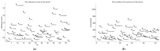
Figure 1.
The distribution of the terms based on (a) the relevance score; (b) the number of occurences.
Terms such as agriculture (332), irrigation (252), soil (357), and agricultural production (406) indicate a major interest in the impact of irrigation on soil, plant growth, and agricultural yield. The presence of the terms climate change (222), temperature (223), and water management (511) shows that research focuses on the influence of climatic conditions on irrigation efficiency. Also, the term wastewater (149) suggests interest in water reuse in agriculture. The use of the terms model (721) and parameter (297) indicates the application of mathematical models for irrigation optimization. Also, the high frequency of case studies (187) and scenarios (213) confirms the use of empirical analyzes and simulations. The occurrence of the words challenge (334), problem (232), and need (246) highlights the current difficulties in water management and the need for more effective solutions. The presence of the terms technology (362) and management (511) suggests an increased interest in solutions based on automation, sensors, and precision agriculture to improve irrigation efficiency. The words sustainability (187) and farmer (123) indicate a concern for the sustainable use of water resources and the impact of agricultural policies on farmers.
As a general trend, the results based on relevance score (the most relevant terms) show that studies in the literature are analyzing the concentration of influence factors, sustainability, technological impact, and global challenges. On the other hand, the results based on the number of occurrences show that the analyzed literature emphasizes models, effects, environmental conditions, development, data, and management.
After the analysis of the obtained terms, we can show the results related to the analysis of the network. Various variants of term maps can be seen in Figure 2.
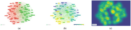
Figure 2.
The term map in three forms: (a) Network visualization. (b) Overlay visualization. (c) Density visualization.
The cluster visualization permits the determination of the two main clusters of terms. The first one, Cluster 1, related to resource management and climate impact, includes terms such as agriculture, climate change, strategy, sustainability, management, and agricultural policies. It focuses on economic, ecological, and public policy approaches to water management in agriculture. Cluster 2, related to modeling, technology, and scientific parameters, includes terms such as model, irrigation, parameter, soil, technology, temperature, and yield. This includes technical approaches based on mathematical modeling, artificial intelligence, and smart irrigation systems. This separation suggests that the optimization of irrigation can be achieved through a combination of management strategies and advanced technological solutions. Recent research is focusing on integrating these two directions to create sustainable and efficient water use systems in agriculture.
The network visualization adds additional criteria related to data analysis and temporal trends. As seen in Figure 2, the trends show that the research initiatives slightly shifted from more general approaches, mainly related to the modeling and analysis of case studies (2018), to the study of the agricultural, botanical, and economical conditions (2019) and smart systems to promote sustainability, food security, and environmental challenge approaches (2020).
The density visualization emphasized terms such as “study,” “effect,” “treatment,” “plant,” “development,” “data,” and “condition”. These reflect essential aspects of irrigation research, focusing on studies and the effects of treatments on plants, the development of technologies and techniques, the use of data to optimize processes, and the external conditions that influence these processes. These terms emphasize the importance of understanding the complex variables that influence irrigation efficiency and water use in agriculture.
As a conclusion, the study conducted highlights the significant links between key terms in the field of irrigation optimization, emphasizing the importance of studies, treatments, and environmental conditions in the development and efficiency of agricultural processes, thus providing a solid basis for future research in the field.
2.4.3. State-of-the-Art Review
In recent years, smart irrigation systems have evolved through the integration of data-driven algorithms, sensor networks, and cloud or edge computing platforms. Deep reinforcement learning (DRL) models have been proposed to autonomously learn irrigation policies under uncertain conditions [34], while fuzzy logic controllers offer rule-based adaptability in multi-objective environments [35]. Internet of Things (IoT)-enabled frameworks, often combining real-time sensing with wireless control, have demonstrated promising field-level results [36].
Moreover, hybrid approaches that couple predictive machine learning models (e.g., LSTM or BPNN) with optimization engines (e.g., PSO, GA, or NSGA-II) have shown improved accuracy in water-use forecasting and irrigation scheduling [37]. These systems often rely on dense sensor arrays or satellite data inputs, and may require computationally intensive model training phases.
In contrast, IRIGEN offers a lightweight and interpretable alternative that avoids the need for large training datasets, and focuses on high spatial resolution and adaptability to grid-based irrigation layouts. The following sections demonstrate how IRIGEN balances computational efficiency with field-level applicability in resource-constrained agricultural contexts.
2.4.4. Methodological Comparison
As for the usage of genetic algorithms for the specific issue described previously, while the recent literature highlights the potential of hybrid and AI-based models like GA–BPNN and DRL for adaptive irrigation, IRIGEN offers a computationally efficient and interpretable alternative that achieves strong performance without requiring extensive training data or complex infrastructure. Table 2 shows a comparison between the IRIGEN, GA-BPNN, and DRL models, as mentioned in the Introduction section.
Table 2.
Comparative evaluation of IRIGEN, GA–BPNN, and DRL models in terms of computational and practical aspects.
In the table, P denotes the population size, G the number of generations, C the cost of evaluating a fitness function, N the number of network parameters, E the number of training epochs, T the number of timesteps per episode, and S the dimensionality of the state space. The comparative table was constructed based on a qualitative synthesis of claims and data reported in the cited literature, as well as the computational and functional characteristics explicitly described for each model. Where direct benchmarks were unavailable, theoretical complexity and typical implementation behavior were used to estimate comparative values.
While IRIGEN offers transparent and efficient control with minimal hardware and no training, GA–BPNN and DRL models provide adaptive capabilities at the cost of increased computational complexity and infrastructure requirements. Each approach offers trade-offs between performance, complexity, and practicality depending on the deployment context.
2.5. Model Description
This section presents the description of the IRIGEN model, based on its purpose, the conceptual and structural model, and the heuristic model which will be used in the implementation of the problem.
2.5.1. Purpose
The purpose of the model is to formulate and solve a combinatorial optimization problem, in which the optimal configuration for activating irrigation points is determined so as to minimize total water consumption, respecting a set of water and spatial constraints. Mathematically, the purpose of such a model is to formulate and solve an optimization problem on a discrete and spatially dependent space, with the objective of controlling the distribution of a limited resource (water) under nonlinear and distance-dependent constraints.
2.5.2. Structural Model of the Irrigation System-IRIGEN-CM1
The structural model of the irrigation system presents the structure of the irrigation system, the conceptual desscription of the layout, and the dynamics of the system. In this matter, the IRIGEN-CM conceptual model is described from the perspective of the system dynamic (IRIGEN-CM1). To improve clarity, the following subsections first present the environmental and simulation input data, then detail the irrigation demand model, and finally describe the optimization algorithm used.
Structure
The main components of the structure of the model were enumerated in the previous sections and the mathematical conceptualization for each component is determined as follows:
- The grid for the agricultural surface: The agricultural area is discretized in the form of a regular two-dimensional grid, composed of square cells of 1 m2, each identified by a pair of indices , where i represents the row (on the x axis) and j the column (on the y axis). Each cell is associated with a unique spatial position in the cartesian system , corresponding to the center of the cell, determined by the following relations:where represents the size of a cell in each direction. Thus, the cell has its center at , and the cell is positioned at coordinates .
- The cell: A cell is characterized by the following parameters:
- –
- Position: —coordinates of the cell in the grid.
- –
- Water status:
- *
- U—current moisture content,
- *
- —normalized moisture content,
- *
- —irrigation input in cell ,
- *
- —water required in cell .
- –
- Meteorological data:
- *
- P—precipitation,
- *
- —potential evapotranspiration,
- *
- —actual evapotranspiration.
- –
- Soil parameters:
- *
- —field capacity,
- *
- —permanent wilting point,
- *
- H—soil depth,
- *
- —volumetric moisture.
- –
- Agronomic parameters:
- *
- —number of plants per cell,
- *
- —root depth or uptake radius.
- –
- Water received from the network:
- *
- —amount of water delivered by emitter k to cell .
- The water distribution system: The exact representation of the position of each irrigation point (tap, sprinkler, dripper, etc.) on an agricultural area is modeled by the transposition of the irrigation point in the cartesian system , correlated to the discretization of the agricultural surface in square units. In this matter, considering the set of irrigation points , each point is characterized by the two coordinates (), where n is the total number of irrigation points. The water distribution system configuration can lead to the assumption that a cell can contain a variable number of irrigation points or an irrigation point can serve a number of cells.
Parameters
The parameters of the model can be clustered in several groups:
- soil and water parameters: each soil used for agriculture has specific characteristics, established by its natural configuration. Related to water, these characteristics refer to the capacity of the soil to retain water. The soil and water parameters are presented in Table 3.
Table 3. Soil and water physical parameters.Table 3. Soil and water physical parameters.
Symbol Description Unit H Depth of the active soil layer m Volumetric mass of the soil t/m3 Field capacity % (by mass) Permanent wilting point % (by mass) Current soil moisture in cell % (by mass) Final soil moisture after irrigation in cell % - Meteorological parameters: The weather conditions on the location of the agricultural surface are essential to the soil water dynamics. The meteorological parameters are presented in Table 4.
Table 4. Meteorological parameters.Table 4. Meteorological parameters.
Symbol Description Unit Daily precipitation in cell mm/m2 Reference evapotranspiration mm/day Actual evapotranspiration in cell mm/day - Water distribution system parameters: The irrigation system has a defined structure with specific parameters. These are presented in Table 5.
Table 5. Water distribution parameters.Table 5. Water distribution parameters.
Symbol Description Unit Irrigation requirement for cell m3/m2 Total daily available water m3/day Maximum number of active irrigation points - - Irrigation points parameters: Each irrigation point is characterized by specific parameters related to position, function, or water flow. These parameters are presented in Table 6.
Table 6. Irrigation point parameters.Table 6. Irrigation point parameters.
Symbol Description Unit Coordinates of irrigation point k in m Distance between irrigation points on the same row m Distance between rows of irrigation points m Irrigation point density: 1/m2 Decision variable: 1 if irrigation point k is active - Individual irrigation flow rate m3/day Water delivered from point k to cell m3 Distance between point k and cell m Water loss coefficient (per distance unit) - - Crop parameters: The crop cultivated on the land also has a massive influence on water budget and necessity. These parameters are presented in Table 7.
Table 7. Crop parameters.Table 7. Crop parameters.
Symbol Description Unit Crop coefficient - Actual crop evapotranspiration: mm/day Distance between plants along the row m Distance between rows m Plant density in cell : 1/m2 Daily water requirement per plant m3/plant/day
To estimate the water requirement of each cell in the field, the model uses a soil water balance approach based on crop and soil properties. The required irrigation volume for cell (i, j) (the basis of the computation) is calculated as:
where:
- is the water requirement for cell [m3];
- is the crop coefficient (dimensionless);
- is the reference evapotranspiration [mm/day];
- H is the effective rooting depth or soil depth [m];
- is the target volumetric soil moisture [m3/m3];
- is the actual soil moisture in cell [m3/m3].
The integration of these parameters allows not only the precise calculation of water demand and supply at the cell level, but also the detailed spatial modeling of the phenomenon, essential for the efficient application of optimization algorithms. Thus, the set of parameters constitutes the mathematical and functional foundation of the entire model.
Relationships
The parameters presented above have a specific behavior and they interact in an integrated environment. We can define relationships between parameters as equations between the main indicators that symbolize those parameters. In this matter, we can group the relationships into four main categories:
- Water budget relationships: These equations determine how much water must be supplied to a cell to keep the soil within a viable agronomic range. Equation (3) shows the central relation, established as the necessary quantity of water in a specific cell. This quantity is needed to restore the soil to field capacity and compensate for losses through evapotranspiration.In order to establish the value of the in the previous equation, its value is calculated using the crop type (represented by ) and the nominal value (calculated using a theoretical formula, such as Penman equation). Equation (4) presents water losses through evaporation and transpiration.Another important relationship related to water budget in the soil is related to the estimated soil water content after irrigation, presented in Equation (5).These relationships are important, as they determine the soil water content and necessary quantity.
- Water distribution relationships: The water distribution system established in the form presented in the structure section shows that there are several relationships between the spatial configuration and the quantity and delivery of the water necessary. In this matter, Equation (6) shows the total quantity of water delivered to a cell from all the irrigation points that are physically present in the respective cell.The next equation (Equation (7)) details the water quantity distributed by a single irrigation point . Several aspects such as irrigation point density and its distance from the center of the cell are taken into consideration.The distance between the irrigation point and the center of the cell in which the point is located is calculated using the Euclidean distance.The density of the irrigation points is also important within the model. It is calculated based on the distance between the irrigation points within the system.The water distribution relationships determine how the distribution system behaves within the integrated irrigation system.
- Water consumption relationships: In order to establish the total consumption within the irrigation system, several elements must be computed. In this matter, Equation (10) shows the total water consumption of the irrigation system, i.e., the sum of the flows from all activated irrigation points.The next equation is related to the density of the plants per cell within the crop, which is established by the agricultural technical aspects.We must also take into consideration the water consumption of the plant. The next equation computes the total water requirement of plants in a cell, i.e., the daily water required by all plants in that cell.This category of relationships is related to water consumption and establishes the dynamics of the consumption, which will be used in contrast with the necessary water quantity.
- Spatial positioning relationships: This relationship calculates the coordinates of the center of a cell in a 2D cartesian grid, assuming that each cell has a dimension of 1 m2.The geometric position is needed to calculate the distances to the irrigation points.
All the presented equations have the role of mathematically modeling the spatial and temporal distribution of water within an irrigation system by quantifying the water demand in each cell, calculating the effective water delivery from irrigation points, evaluating soil moisture, and optimizing irrigation points activation, taking into account hydrological, physical, and agronomic constraints.
Restrictions
The constraints formulated within the irrigation model play an essential role in guaranteeing the technical feasibility and agronomic validity of the generated solutions. There are three restrictions used within the model.
The first restriction (minimum water content constraint), shown in Equation (14), ensures that after irrigation, the soil moisture in cell remains high enough to support the plants, i.e., above the permanent wilting point () and covers the daily water requirement of the plants.
The second restriction (maximum water content constraint), shown in Equation (15), prevents soil overloading with water beyond field capacity (FC), which could lead to losses through percolation, soaking, and impaired root development.
The third restriction (total water consumption constraint), shown in Equation (16), is related to water efficiency. At the global level, the constraint on the total amount of water available reflects the real limits of the resource and imposes a trade-off between spatial demand and system availability, directly contributing to water use efficiency.
Together, these constraints ensure that the model not only works mathematically correctly, but also respects the ecological, technical, and economic requirements of a modern irrigation system.
2.5.3. Optimization Model-IRIGEN-CM2
The model minimizes the total volume of irrigation water used by selecting an optimal subset of irrigation points to activate, such that each cell receives sufficient water to satisfy soil and crop requirements without exceeding physical and agronomic constraints, and respecting a daily water budget. Thus, we will formulate the mathematical model of the optimization problem using a classical approach: parameter definition, objective function, and constraints.
Decision variables:
Objective function:
Subject to:
- Water availability constraint:
- Minimum moisture constraint:
- Maximum moisture constraint:
Parameters
The main parameter of the optimization model is the irrigation points array, in the form of a binary decision variable array indicating whether irrigation point k is active (1) or not (0):
In this matter, the variable array determines whether an irrigation point contributes to the global efficiency.
Objective Function
The objective function minimizes the total water used by the active irrigation points, as shown in Equation (18).
This represents the total volume of irrigation water used, in m3/day. The optimization function aims to minimize total water consumption by activating an optimal subset of irrigation points, so as to ensure that the water needs of the plants are covered and that physical–agronomic and resource constraints are respected.
Constraints
The constraints are related to the soil physical capacity of water budget and the available water quantity for irrigation. In this matter, the next constraint ensures that the final soil water in each cell is sufficient to avoid plant water stress.
The following constraint prevents over-irrigation by requiring that soil water not exceed field capacity.
Finally, the global water usage constraint limits the total volume of water used in a day so that the available daily resource of the irrigation system is not exceeded.
These constraints have the role of ensuring the applicability of the solutions generated by the optimization model, maintaining the balance between plant needs, the physical capabilities of the soil, and the limits of the irrigation system.
2.5.4. Heuristic Model of the Irrigation System-IRIGEN-GM
Components
The heuristic model is obtained by transposing the IRIGEN-CM model using genetic methods and techniques with the purpose of obtaining an implementation using a genetic algorithm. In this matter, the following elements are taken into consideration:
- The gene g: A gene represents the state (active/inactive) of an irrigation point, where 1 represents the active state and 0 the inactive state of the irrigation point:
- The chromosome C: A chromosome is a sequence of genes that form a complete solution (a configuration of activated irrigation points):
- The fitness function f: Evaluates how “good” a solution (chromosome) is relative to the objective and constraints of the model. Its value is presented in the following equation:where
- –
- is the number of cells with lower water content than PWP on the entire surface;
- –
- is the number of cells with higher water content than CC on the entire surface;
- –
- are the dimensions of the grid (the total number of cells within the entire surface, equal to the number of m2 of the entire surface).
The fitness function used in IRIGEN jointly minimizes both deficit and surplus of irrigation, while penalizing excessive resource use. It implicitly adapts to varying environmental and agronomic conditions by accounting for spatial soil moisture distributions, plant-specific water requirements (), evapotranspiration (), and infiltration dynamics.In addition, the function incorporates a distance-attenuated irrigation effect through the term , which reduces the influence of irrigation points based on their distance to the target cell. Components of the fitness function are normalized to the interval to ensure balanced contribution and prevent any single term from dominating the optimization process. This makes it adaptive to the spatial configuration and hydrological context of the grid.The weights used for these components were chosen empirically to balance their influence and to prevent dominance of a single term in the optimization process. However, all terms are normalized to ensure comparability, and their combined effect is aligned with precision agriculture principles. - The genetic parameters : The set of genetic parameters used for the implementation. This is a tuple of four parameters (), where is the initial population size, is the number of generations, is the mutation rate, and is the crossover rate.
- The genetic operators: The genetic operators are responsible for the variation of the population. These are a s follows:
- –
- Mut: The mutation operator, equivalent to swapping a randomly chosen gene value.
- –
- Crs: The crossover operator, used to obtain a new chromosome by selecting two parents to produce an offspring. A crossover point is chosen randomly and the two chromosomes are merged based on the crossover point.
- –
- Sel: The selection operator, which selects chromosomes with better fitness for reproduction. A sorting selection is used, a fixed number of the best chromosomes being used for the next generation.
The methodology can be viewed schematically in Figure 3.
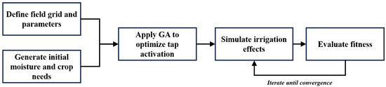
Figure 3.
A visual representation of the methodology.
The proposed genetic model provides a flexible and robust framework for exploring the space of possible solutions, allowing the identification of efficient irrigation configurations that respect agronomic constraints and resource limits, while optimizing water consumption at a spatial scale.
The Genetic Algorithm
The genetic algorithm presented below (Algorithm 1) is used to optimize the activation of irrigation points, aiming to minimize total water consumption under physical–agronomic constraints.
| Algorithm 1 Genetic Algorithm for Irrigation Optimization |
|
At the end of the iterations, the algorithm returns the optimal chromosome , which corresponds to the best solution identified in the set of evaluated populations.
2.5.5. Model Example
To illustrate a potential deployment, consider a tomato greenhouse of 500 m2, structured in 25 planting rows spaced at 0.8 m, each containing drip irrigation lines with emitters placed every 0.3 m. Each emitter supplies up to 2 L/h, and the total number of irrigation points reaches approximately 2000. The IRIGEN model could operate based on daily weather data (temperature, humidity, solar radiation) and basic soil sensors (e.g., 6–8 distributed probes for soil moisture and temperature). Based on plant density (3–4 plants/m2) and a daily crop evapotranspiration of 4–5mm/day during peak season, the system would estimate per-cell demand and optimize emitter activation under a capped water allocation (e.g., 1.2 m3/day).
For the given example, the following components are required for the practical deployment of the IRIGEN model in a greenhouse setting:
- Cultivation area: Greenhouse with a discretizable surface (e.g., 500 m2), divided into 1 m2 grid cells.
- Irrigation system: Emitter-based drip irrigation with approximately 2000 individual points, installed along rows spaced at 0.8 m.
- Soil sensors: Minimum of 6–8 soil moisture probes distributed spatially, optionally including temperature or salinity measurements.
- Weather input: Daily meteorological data such as air temperature, humidity, solar radiation, and wind speed, used to compute .
- Computational unit: Local processor (e.g., laptop, Raspberry Pi) running the IRIGEN algorithm and determining optimal irrigation points.
- Irrigation control interface (optional): electronic valve controllers or relay boards to automate emitter activation, optionally integrated with an IoT platform (e.g., Node-RED).
This setup highlights IRIGEN’s potential to support precise irrigation control with minimal hardware and no training data, compared to deep learning models. Moreover, the greenhouse context allows partial automation and integration with IoT devices (e.g., timers, valves), bridging the gap between theoretical optimization and real-world use in controlled horticultural environments.
3. Results
3.1. Initial Setup
The initial configuration defines the baseline conditions for evaluating the performance of the irrigation optimization process. The system under study consists of a rectangular agricultural field discretized into a uniform grid of square cells, each representing an area of . Each cell has a predefined water demand, assumed to be spatially heterogeneous, but bounded within realistic agricultural limits. This configuration can be seen in Figure 4.
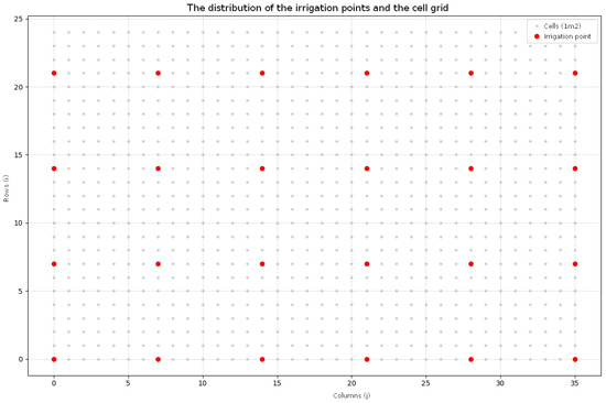
Figure 4.
Grid layout and irrigation points placement for the test scenario points.
The field configuration, crop parameters, and soil moisture values used in this study are synthetically generated, based on realistic agricultural data drawn from the literature. The scenario is simulated in the absence of experimental field measurements. The parameters used in the simulation are based on standard agronomic and environmental values. While no real-time sensor data are used, the IRIGEN framework includes dynamically generated spatial soil moisture distributions and considers daily evapotranspiration, infiltration, and plant-specific coefficients. These simulate realistic environmental dynamics and make the model adaptable to real-world variability.
The simulation is based on realistic but synthetic data to ensure controlled evaluation of the proposed method. Soil parameters such as field capacity (CC = 0.35), permanent wilting point (PWP = 0.15), and soil depth (H = 0.3 m) were adopted from representative loamy soil conditions, consistent with FAO guidelines. The reference evapotranspiration ( mm/day) and crop coefficient () reflect typical mid-season conditions for high water-demand crops. The available irrigation flow per point ( m3/h) is assumed based on low-pressure localized systems, operating 6 h/day. The environmental and agronomic parameters used (e.g., soil properties, crop coefficients, ) reflect values typical for temperate-climate regions in Southern and Eastern Europe (e.g., Romania).
A total of 24 potential irrigation points (taps) are distributed across the field. Each tap has a fixed maximum delivery capacity and a known irrigation footprint, affecting multiple surrounding cells depending on its location and activation status.
Table 8 summarizes the genetic algorithm parameters used in the IRIGEN model, along with the rationale behind each choice. The settings were selected empirically to balance solution quality, convergence speed, and computational cost in a spatial optimization context. Although the genetic algorithm used in IRIGEN follows a standard formulation, its tailored application to spatial irrigation control—through binary chromosome encoding of tap activation and a composite fitness function reflecting agronomic constraints—leads to superior performance in water use efficiency.
Table 8.
Genetic algorithm hyperparameters and their justification.
A formal sensitivity analysis of the GA hyperparameters was not performed in this study; however, future work will explore systematic tuning procedures (e.g., grid search) to evaluate robustness across different environmental conditions. Future extensions of IRIGEN will include a formal sensitivity analysis of the genetic algorithm hyperparameters, based on a factorial design over parameter ranges (e.g., population size, mutation, and crossover rates). Each configuration will be evaluated through multiple independent runs to assess convergence stability, solution quality, and computational efficiency. This will allow us to identify robust parameter settings and understand the impact of each hyperparameter on irrigation performance metrics such as water surplus, deficit, and spatial uniformity.
3.2. Results for the Scenarios
3.2.1. Baseline Scenario
In the reference scenario,
- All 24 irrigation points are considered active by default.
- Water is distributed uniformly from each active tap, without optimization or selection, based on demand patterns.
- The objective function evaluates system performance based on three key criteria:
- Water deficit—the shortfall between delivered and required water per cell.
- Water surplus—the excess water beyond what each cell requires.
- Total water consumption (Qtotal)—the overall volume used.
In the baseline scenario, all 24 irrigation points are simultaneously active across the grid, representing a non-optimized, full-activation configuration. Water is distributed uniformly without accounting for spatial variability in soil moisture or crop demand. This approach results in excessive water use, with total consumption exceeding 10 m3. The computed fitness value for this configuration is −0.1503, indicating a suboptimal balance between water deficit and surplus. While average deficit and surplus values per cell are not minimized, they are estimated to be higher than those obtained in the optimized configuration, highlighting inefficient water distribution. The Deficit Coverage Rate (DCR) is presumed to be above zero, meaning that not all crop water demands are met despite high resource usage. The Water Stress Index (WSI) in this case is undefined but assumed to be high, reflecting uneven and excessive irrigation. This baseline serves as a reference for evaluating the performance improvements achieved by the IRIGEN optimization model.
3.2.2. Optimized Scenario (IRIGEN)
The values of the deficit, the surplus, and the total soil water content are shown in Figure 5.
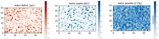
Figure 5.
Deficit, surplus, and humidity U′.
The optimal solution identified by the algorithm is represented by the following chromosome:
[0, 1, 1, 0, 1, 1, 1, 1, 0, 0, 0, 1, 1, 0, 0, 1, 1, 1, 0, 1, 1, 1, 0, 1, 1, 1]
The visual representation of the solution and the value of the water delivered in the cells is shown in Figure 6.
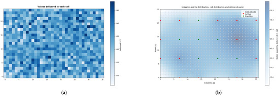
Figure 6.
Visual representation of the solution: (a) Values delivered in cells. (b) Distribution of active/inactive irrigation points and water delivered.
This sequence defines the activation status of the 24 available irrigation points, where 1 indicates an active tap and 0 an inactive one. The corresponding configuration yielded a fitness score of −0.0814, which is a substantial improvement over the reference scenario value of −0.1503. This reflects an approximate 46% increase in solution quality.
3.3. Comparative Analysis
The comparison between the effects of the two scenarios can be visualized in Table 9.
Table 9.
Comparison between baseline (full activation) and optimized IRIGEN scenario.
Table 9 highlights the superior performance of the IRIGEN model, which reduces water consumption by over 50% compared to the full activation scenario, maintaining a zero deficit and significantly lower water stress.
3.4. Fitness Analysis
The fitness function used for evaluation combines these three aspects into a single scalar value, which the genetic algorithm attempts to minimize. The fitness value for this unoptimized baseline configuration (reference scenario) was computed as . This scenario serves as a benchmark against which the algorithmically optimized solutions are compared. Any improvement beyond this value indicates better spatial water efficiency, reduced waste, or more targeted irrigation delivery. The behavior of the fitness is shown in Figure 7.
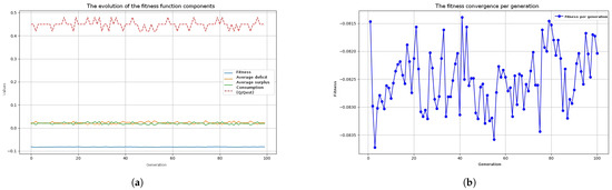
Figure 7.
Fitness behavior: (a) Evolution of fitness function components. (b) The convergence of fitness across generations.
The genetic algorithm effectively identified an optimal configuration that minimizes both water deficit and surplus, reduces overall water consumption, and achieves complete coverage of irrigation needs. Notably, this was accomplished with a minimized number of active points, underlining the algorithm’s capacity to optimize resource allocation and operational efficiency in irrigation system design.
4. Discussion
At the conclusion of the evolutionary process, the genetic algorithm succeeded in generating a solution that is significantly improved compared to the reference scenario. The key performance metrics recorded at generation 100 are summarized below:
- Fitness function value: −0.0820, indicating a well-balanced solution with respect to minimizing water deficit, surplus, and overall water usage.
- Total water volume delivered (Qtotal): 4.5000 m3, efficiently distributed across the entire surface area.
- Average water deficit: 0.0221 m3 per cell—a low value that reflects effective coverage of irrigation demand.
- Average water surplus: 0.0190 m3 per cell—suggesting that over-irrigation was successfully avoided.
- Deficit Coverage Rate (DCR): 0.0000, confirming that all cells received their full water requirements.
- Water Stress Index (WSI): 0.3320, which indicates low stress levels and good uniformity in water distribution.
The results clearly demonstrate that the IRIGEN model significantly outperforms the full-activation baseline in terms of water efficiency and irrigation quality. By activating only 17 out of 26 available irrigation points, the optimized solution achieved complete coverage of crop water requirements (DCR = 0) while reducing total water use by more than 50%. This outcome suggests that a strategic, spatially informed activation of taps—driven by genetic optimization—can drastically reduce overuse and improve precision without sacrificing irrigation effectiveness. The drop in the fitness value from −0.1503 to −0.0814, coupled with minimized surplus and deficit indicators, highlights a well-balanced trade-off between resource savings and agronomic needs.
The average surplus of 0.019 m3/cell observed in the optimized IRIGEN scenario was not a preset design value, but emerged from the GA optimization under constraints of zero deficit (DCR = 0) and low water stress (WSI). While this corresponds to roughly two days of peak crop water demand, for the loam soil in this study (AW = 60 mm) it represents 31.7% of the available water—above the 10–15% range typically recommended by FAO-56. To assess the agronomic validity of this surplus, we compared it to the reference band for a set of soil–crop combinations, as shown in Table 10.
Table 10.
Comparison of the optimized surplus OS (0.0190 m3/cell) with FAO-56 reference range (10–15% of AW) for various soil–crop combinations.
The results indicate that the optimized surplus exceeds the FAO-56 10–15% AW reference range in most soil–crop scenarios, including the loam soil of this study. Only the clay loam with deep-rooted crops (alfalfa) meets the reference threshold. The higher proportion in the optimized case is attributable to the simulated distribution non-uniformity and peak evapotranspiration demand, suggesting that while the surplus is operationally minor in absolute terms, it is relatively high in proportion to AW. This highlights the need for context-specific recalibration to minimize deep percolation losses in other soil–crop–climate conditions.
Unlike most conventional irrigation optimization models, which often rely on black-box machine learning techniques (e.g., BPNN or DRL), the IRIGEN model emphasizes algorithmic transparency, spatial resolution, and minimal data requirements. While genetic algorithms have previously been used in irrigation planning, IRIGEN differs in the way it integrates spatially distributed constraints, field-scale emitter mapping, and soil–plant feedback directly into the fitness function.
To highlight its advantages, we compared IRIGEN with recent peer models such as GA-BPNN hybrid systems and DRL-based controllers, as summarized in Table 2. IRIGEN achieves lower computational complexity () and does not require training data, making it more suitable for deployment in data-scarce environments. Furthermore, its interpretability and modularity allow easier integration with sensor-based decision platforms in practical deployments.
To further contextualize IRIGEN’s performance, Table 11 presents a comparative summary with recent studies applying genetic algorithms for grid-based or spatially explicit irrigation optimization. The comparison includes computation time, water-saving efficiency, and the standard deviation of irrigation uniformity or efficiency, where available. These metrics provide a quantitative benchmark, clarifying IRIGEN’s computational efficiency and water-saving potential relative to peer methodologies.
Table 11.
Comparative performance of GA-based irrigation optimization studies. Studies prior to 2022 are marked as older benchmarks.
The values in Table 11 were obtained based on recent studies on optimization through genetic algorithms in irrigation and water distribution networks [38,39,40,41]. In short, IRIGEN has performances related especially to water efficiency and uniformity, even if the calculation time is longer than other studies focused on smaller networks or with reduced NG. This comparative framing helps highlight IRIGEN’s competitive efficiency and adaptability, while acknowledging variations in experimental conditions and metrics.
While IRIGEN integrates a diverse set of agronomic, soil, and meteorological inputs, no formal sensitivity analysis has been conducted to assess the relative influence or potential redundancy of these parameters. Future work will include parameter importance ranking, potentially using variance-based techniques or permutation importance, to identify dominant factors and simplify the model without compromising accuracy.
In order to show an example of an analysis that will be made using specific data from future work, a theoretical sensitivity estimation using representative values from the agronomic literature is shown next. It suggests that several parameters disproportionately influence the water requirement per cell. For instance, assuming a tomato crop grown in a greenhouse with , , and a soil depth , the crop evapotranspiration reaches:
Using the soil water balance equation (Equation (3)) and typical values , , , the irrigation need becomes:
A plus or minus 10% change in , , or H yields:
This translates to a 9%–10% change in daily water requirement, showing high sensitivity to crop and climatic parameters. In contrast, varying or within realistic bounds (plus or minus 10%) produces smaller absolute changes (under 0.5 mm/day), indicating moderate sensitivity.
These estimates suggest prioritizing precision in measuring , , and H when calibrating the model or deploying in the field.
Further, an empirical sensitivity analysis was made and the results are shown in Table 12. The sensitivity analysis evaluated the impact of four core genetic algorithm parameters—population size (NP), number of generations (NG), mutation rate (rm), and crossover rate (rc)—on convergence behavior, solution quality, and computational cost. Each configuration was run twice, and average values were computed for best fitness, convergence generations, execution time, water stress index (WSI), deficit coverage ratio (DCR), total applied water volume (Qtotal), and water use reduction relative to full activation.
Table 12.
Aggregated sensitivity analysis results for GA parameters (average over two repetitions), ordered by NP, NG, rm, rc.
The results indicate that all tested parameter combinations yield similar best fitness values (variation < 0.002), confirming the robustness of IRIGEN’s optimization. However, execution time is strongly affected by NP and NG, with the largest configuration (NP = 100, NG = 100) requiring up to five times longer than the smallest (NP = 50, NG = 60) for negligible fitness gains. Mutation and crossover rates had minor influence on WSI and Qtotal, suggesting that moderate values (rm = 0.05–0.10, rc = 0.4–0.7) maintain performance while controlling computation time.
From a methodological perspective, the genetic algorithm proved effective in navigating a large and complex solution space, identifying a configuration that simultaneously minimizes three conflicting objectives: deficit, surplus, and consumption. The model’s robustness stems from its binary chromosome representation and carefully tuned hyperparameters, enabling convergence within a reasonable number of generations. Although the simulation relies on synthetic data, the underlying logic reflects realistic agronomic principles and supports adaptation to field conditions. Compared to more complex hybrid approaches such as fuzzy-GA, BPNN-based prediction models, or deep reinforcement learning schedulers, IRIGEN offers a simpler and interpretable alternative that achieves substantial water savings without requiring large datasets or real-time sensor integration. These findings validate the feasibility of grid-based, algorithmic irrigation optimization and set the stage for future integration with real-time sensor data, IoT systems, or adaptive multi-objective frameworks.
To complement the visualization of irrigation distribution (e.g., in Figure 5 and Figure 6a), a quantitative assessment of spatial uniformity may be introduced in future work. Metrics such as the Coefficient of Variation (CV), Distribution Uniformity (DU), and Root Mean Squared Deviation (RMSD) between achieved vs. required soil moisture could be computed for each algorithm. These would offer a more robust comparison of irrigation effectiveness and consistency.
For instance, the Distribution Uniformity (DU) index:
is widely used in irrigation system design and can quantify over- or under-irrigation zones.
Heatmaps may then be accompanied by pixel-wise error maps or delta distributions (e.g., ) to highlight areas of surplus or deficit. Such comparative visualizations and error metrics could reveal not only total water efficiency but also fairness in water allocation across the field.
In the current study, visual patterns suggest that IRIGEN provides more consistent moisture coverage with minimal over-irrigation zones, but further validation using these uniformity metrics is recommended.
While the presented results emphasize overall water efficiency (e.g., over 50% reduction compared to full-field irrigation), the analysis does not explicitly account for the impact of parameter fluctuations or environmental extremes. Future work will incorporate sensitivity analyses by simulating variable climate scenarios, such as prolonged drought (e.g., elevated , reduced P) or sudden rainfall events. These scenarios will assess how robust the IRIGEN optimization remains under stress conditions.
In addition, error sources such as sensor inaccuracy, spatial soil heterogeneity, or model parameter uncertainty (e.g., or H) may affect irrigation precision. Their potential impact can be quantified by perturbing key inputs and measuring variance in fitness or water use. This would enable a more comprehensive understanding of model reliability under realistic field conditions.
In order to assess how this sensitivity analysis to parameter fluctuations or environmental extremes will be developed in future work, we can start by simulating the sensitivity of the model to climatic fluctuations. For this, we start by simulating three scenarios using the core irrigation demand formula (Equation (3)).
Assuming the following constant soil parameters:
- , , ,
- Crop coefficient
We compute the irrigation requirement for three climate cases in the next Table (Table 13).
Table 13.
Irrigation demand under variable climate scenarios.
The results show that a dry scenario increases water demand by approximately 31% compared to baseline, while heavy rainfall can reduce it by 45%. These significant shifts highlight the necessity of incorporating climate-aware strategies or real-time data sources to maintain irrigation efficiency.
5. Conclusions
This paper presented an optimized irrigation model based on a grid of cells, using an evolutionary algorithm for valve control. The results obtained indicate an efficient water distribution, with a reduction in the differences between the water demand and delivery in each cell.
Under the simulated field conditions, the IRIGEN model reduced total water use by more than 50% compared to full activation. The optimized configuration covered all plant water needs with no deficit (DCR = 0) and minimal surplus (average = 0.019 m3). According to FAO Irrigation and Drainage Paper No. 56, typical crop water requirements in hot, dry climates can reach 10 mm/day (i.e., 10 L/m2/day) [42]. Therefore, the surplus observed in our simulations corresponds to nearly twice the daily crop water demand, and may be agronomically significant if not justified. However, FAO-56 also states that minor excess volumes are often acceptable or even necessary for leaching salts and achieving uniform application [42]. Such surplus should be evaluated case by case depending on soil salinity, drainage conditions, and irrigation frequency. While the average surplus of 0.019 m3/cell appears minor when expressed as approximately two days of peak crop water demand, it represents 31.7% of the available water (AW = 60 mm) for the loam soil and rooting depth in this study—above the 10–15% range typically recommended by FAO-56 for standard conditions. This value was not a preset target but emerged from the GA optimization under constraints of zero deficit and low water stress. The higher proportion relative to AW is attributable to the simulated distribution non-uniformity and high peak evapotranspiration rates. Under different soil–crop–climate conditions, recalibration of the surplus would be advisable to prevent deep percolation losses.
A potential direction for future validation involves the use of field-deployable soil moisture sensors (e.g., Decagon 5TE) to monitor real-time water dynamics, as well as remote sensing-based evapotranspiration estimates derived from NDVI indices (e.g., Sentinel-2 imagery). These tools would enable assessment of both spatial uniformity and temporal accuracy of the irrigation configurations generated by the model under real-world conditions.
However, the model presents several limitations that should be addressed in future developments:
- It assumes temporally invariant environmental conditions, with fixed weather inputs (e.g., precipitation, evapotranspiration) and no seasonal dynamics.Future direction: Extend the model to support multi-step simulations or rolling horizons with updated environmental inputs.
- It does not simulate lateral water redistribution between adjacent cells, thereby ignoring infiltration spread or capillary movement.Future direction: Couple with a simple hydrological sub-model or implement a local redistribution matrix.
- The model uses uniform soil and plant parameters across the entire grid, neglecting known spatial heterogeneity in real fields.Future direction: Integrate spatially distributed soil data or crop-specific coefficients from remote sensing or sensor networks.
- Optimization is static and single-step, lacking real-time feedback or historical learning.Future direction: Introduce adaptive optimization or reinforcement learning to respond to environmental changes.
- Field validation is lacking, as current results are based solely on synthetic simulation scenarios.Future direction: Validate the model using field-collected sensor data (e.g., soil moisture probes) or compare against remote sensing estimates (e.g., Sentinel-2 NDVI-based ET).
- The model does not quantify the sensitivity to input parameter uncertainty (e.g., ET0, rainfall, crop coefficients).Future direction: Perform a structured sensitivity analysis (e.g., Sobol, Monte Carlo) to identify key influencing factors and improve robustness.
Despite these limitations, the IRIGEN model demonstrates the feasibility of optimizing irrigation in a grid-based system under realistic spatial variability. Its structure is designed for integration with future IoT and real-data-driven systems. A promising future direction involves integrating IRIGEN with IoT-based irrigation infrastructure, leveraging real-time data from soil moisture sensors and weather stations. Such integration would allow dynamic updates of environmental inputs and more responsive control, enhancing the system’s practicality for precision agriculture applications.
In the future, the model can be extended with dynamic data from sensors, weather forecasts, multi-objective optimization, and real-world field testing. These improvements could significantly increase the practical applicability of the system in precision agriculture.
Supplementary Materials
The following supporting information can be downloaded at: https://www.mdpi.com/article/10.3390/technologies13080366/s1, Table S1: Table of Symbols and Units.
Author Contributions
Conceptualization, D.A.P. and N.B.; methodology, N.B. and A.S.; software, N.B.; validation, D.A.P., A.S. and I.A.P.; formal analysis, N.B.; investigation, D.A.P. and A.S.; resources, I.A.P.; data curation, N.B.; writing—original draft preparation, D.A.P.; writing—review and editing, N.B.; visualization, I.A.P. and A.S.; supervision, D.A.P.; project administration, D.A.P.; funding acquisition, D.A.P. All authors have read and agreed to the published version of the manuscript.
Funding
This research received no external funding.
Institutional Review Board Statement
Not applicable.
Informed Consent Statement
Not applicable.
Data Availability Statement
Data is contained within the article or Supplementary Material.
Conflicts of Interest
The authors declare no conflicts of interest.
Abbreviations
The following abbreviations are used in this manuscript:
| AW | Available Water |
| BPNN | Backpropagation Neural Network |
| CC | Field Capacity |
| CU | Christiansen’s Uniformity Coefficient |
| CV | Coefficient of Variation |
| DCR | Deficit Coverage Ratio |
| DRL | Deep Reinforcement Learning |
| DU | Distribution Uniformity |
| ET0 | Reference Evapotranspiration |
| GA | Genetic Algorithm |
| H | Rooting Depth |
| IoT | Internet of Things |
| IRIGEN | IRrigation via GENetic algorithm |
| LSTM | Long Short-Term Memory |
| NDVI | Normalized Difference Vegetation Index |
| NG | Number of Generations |
| NP | Number of Population |
| PWP | Permanent Wilting Point |
| SOP–WDN | Smart Optimization Program for Water Distribution Networks |
| SWM | Soil Water Management |
| Standard Deviation of Applied Water Volumes | |
| WUE | Water Use Efficiency |
| WSI | Water Stress Index |
References
- Tita, V.; Bozga, I.; Nijloveanu, D.; Vanatoru, D. Research regarding the theoretical knowledge of management held by rural entrepreneurs from SW Oltenia Region. Ann. Univ. Craiova-Agric. Mont. Cadastre Ser. 2014, 43, 226–230. [Google Scholar]
- Singh, A. Irrigation planning and management through optimization modelling. Water Resour. Manag. 2014, 28, 1–14. [Google Scholar] [CrossRef]
- Verhoef, A.; Egea, G. Soil Water and Its Management. In Soil Conditions and Plant Growth; Blackwell Publishing Ltd.: Hoboken, NJ, USA, 2013; pp. 269–322. [Google Scholar]
- Datta, S.; Taghvaeian, S.; Stivers, J. Understanding Soil Water Content and Thresholds for Irrigation management. In Oklahoma Cooperative Extension Service; Oklahoma State University: Stillwater, OK, USA, 2017; Volume 1537, Available online: https://openresearch.okstate.edu/bitstreams/9465ba33-0677-4818-8075-c8b4e263aa15/download (accessed on 25 November 2024).
- Nijloveanu, D.; Bozga, I.; Tita, V.; Vanatoru, D. Soil degradation in Olt County by the process of hydric erosion. Ann. Univ. Craiova-Agric. Mont. Cadastre Ser. 2014, 43, 243–246. [Google Scholar]
- Florea, C.; Burghiu, A.; Ivanovici, M. Logit-Based Superpixel Semantic Segmentation of Images for Precision Agriculture. UPB Sci. Bull. Ser. C 2024, 86, 157–168. [Google Scholar]
- Darshana; Pandey, A.; Ostrowski, M.; Pandey, R. Simulation and optimization for irrigation and crop planning. Irrig. Drain. 2012, 61, 178–188. [Google Scholar] [CrossRef]
- Bostan, A.; Dobrescu, R.; Hossu, D.; Hossu, A. Designing a Fuzzy Controller for the Automation of an Irrigation System. UPB Sci. Bull. Ser. C 2023, 85, 65–76. [Google Scholar]
- Popescu, D.A.; Bold, N. System of monitoring the irrigation of an agricultural surface. In Proceedings of the The 9 th International Conference On Virtual Learning Models and Methodologies Technologies Software Solutions, Bucharest, Romania, 24–25 October 2014; pp. 373–378. [Google Scholar]
- Rani, M.U.; Kamalesh, S. Web Based Service to Monitor Automatic Irrigation System for the Agriculture Field Using Sensors. In Proceedings of the Advanced in Electrical Engineering (ICAEE) 2014 International Conference, Vellore, India, 9–11 January 2014; p. 2. [Google Scholar]
- Ussain, R.; Sahgal, J.L.; Gangwar, A.; Riyaj, M. Control of Irrigation Automatically By Using Wireless Sensor Network. Int. J. Soft Comput. Eng. 2013, 3, 1. [Google Scholar]
- Rasin, Z.; Hamzah, H.; Aras, M.S.M. Application and Evaluation of High Power Zigbee Based Wireless Sensor Network in Water Irrigation Control Monitoring System. In Proceedings of the 2009 IEEE Symposium on Industrial Electronics and Applications (ISIEA), Kuala Lumpur, Malaysia, 4–6 October 2009. [Google Scholar]
- Atodaria, V.H.; Tailor, A.M.; Shah, Z.N. SMS Controlled Irrigation System with Moisture Sensors. Indian J. Appl. Res. 2013, 3, 30–40. [Google Scholar] [CrossRef]
- Harishankar, S.K.U.V.S.; Kumar, R.S.; Sudharsan, K.P.; Vignesh, U.; Viveknath, T. Solar Powered Smart Irrigation System. Adv. Electron. Electr. Eng. 2014, 4, 341–346. [Google Scholar]
- Cosma, D.I.; Andonie, S. Transducers; CD Press Publishing: Bucharest, Romania, 2011. [Google Scholar]
- Marcuzzo, F.F.N.; Wendland, E.C. The Optimization of irrigation networks using genetic algorithms. J. Water Resour. Prot. 2014, 6, 1124–1138. [Google Scholar] [CrossRef]
- González Perea, R.; Camacho Poyato, E.; Montesinos, P.; Rodríguez Díaz, J.A. Optimization of irrigation scheduling using soil water balance and genetic algorithms. Water Resour. Manag. 2016, 30, 2815–2830. [Google Scholar] [CrossRef]
- Gao, X.; Wu, P.; Zhao, X.; Wang, J.; Shi, Y. Effects of land use on soil moisture variations in a semi-arid catchment: Implications for land and agricultural water management. Land Degrad. Dev. 2014, 25, 163–172. [Google Scholar] [CrossRef]
- Victor, T.; Daniel, N.; Popescu, D.A.; Bold, N. Study on the efficiency of the design of the drip irrigation management system using plastics. J. Intell. Fuzzy Syst. 2022, 43, 1697–1705. [Google Scholar] [CrossRef]
- Tita, V.; Bold, N.; Tudor, V.C.; Marcuta, A.; Marcuta, L. The determination of plastic material and the optimal irrigation characteristics for an agricultural surface-model description. Preprints 2020. [Google Scholar] [CrossRef]
- Wang, X. The artificial intelligence-based agricultural field irrigation warning system using GA-BP neural network under smart agriculture. PLoS ONE 2025, 20, e0317277. [Google Scholar] [CrossRef]
- Gaitan, N.C.; Batinas, B.I.; Ursu, C.; Crainiciuc, F.N. Integrating Artificial Intelligence into an Automated Irrigation System. Sensors 2025, 25, 1199. [Google Scholar] [CrossRef]
- Oğuztürk, G.E.; Caner, M.; Yurtseven, M.; Oğuztürk, T. The Effects of AI-Supported Autonomous Irrigation Systems on Water Efficiency and Plant Quality: A Case Study of Geranium psilostemon Ledeb. Plants 2025, 14, 770. [Google Scholar] [CrossRef] [PubMed]
- Lu, H.; Huang, G.; Lin, Y.; He, L. A Two-Step Infinite α-Cuts Fuzzy Linear Programming Method in Determination of Optimal Allocation Strategies in Agricultural Irrigation Systems. Water Resour. Manag. Int. Journal, Publ. Eur. Water Resour. Assoc. (EWRA) 2009, 23, 2249–2269. [Google Scholar] [CrossRef]
- Mekonen, B.M. Integrating AI and Remote Sensing in Precision Agriculture for Advancing Sustainable Irrigation Monitoring and Management in Ethiopia. Am. J. Artif. Intell. 2025, 9, 22–29. [Google Scholar] [CrossRef]
- Saikai, Y.; Peake, A.; Chenu, K. Deep reinforcement learning for irrigation scheduling using high-dimensional sensor feedback. PLoS Water 2023, 2, e0000169. [Google Scholar] [CrossRef]
- British Columbia Ministry of Agriculture, Food and Fishery. Sprinkler Irrigation Scheduling Using a Water Budget Method; Revised May 2004; 2004; p. 2. Available online: https://agwaterstewards.org/wp-content/uploads/2016/08/Water-Budget-Method-of-Irrigation-Scheduling.pdf (accessed on 25 November 2024).
- British Columbia Ministry of Agriculture, Food and Fishery. Soil Water Storage Capacity and Available Soil Moisture; Revised May 2004; 2004; pp. 2–3. Available online: https://www.droughtmanagement.info/literature/BC_MA_Soil_Water_Storage_Capacity_2005.pdf (accessed on 25 November 2024).
- Tudor, V. Optimal Loss Reduction of Distribution Networks Using a Refined Genetic Algorithm. UPB Sci. Bull. Ser. C 2010, 72, 29–38. [Google Scholar]
- Delirhasannia, R.; Sadraddini, A.; Nazemi, A.; Farsadizadeh, D.; Playán, E. Dynamic model for water application using centre pivot irrigation. Biosyst. Eng. 2010, 105, 476–485. [Google Scholar] [CrossRef]
- Reca, J.; Roldán, J.; Alcaide, M.; López, R.; Camacho, E. Optimisation model for water allocation in deficit irrigation systems: I. Description of the model. Agric. Water Manag. 2001, 48, 103–116. [Google Scholar] [CrossRef]
- Hook, D.W.; Porter, S.J.; Herzog, C. Dimensions: Building Context for Search and Evaluation. Front. Res. Metr. Anal. 2018, 3, 23. [Google Scholar] [CrossRef]
- Van Eck, N.J.; Waltman, L. Software survey: VOSviewer, a computer program for bibliometric mapping. Scientometrics 2010, 84, 523–538. [Google Scholar] [CrossRef] [PubMed]
- Yang, Y.; Hu, J.; Porter, D.; Marek, T.; Heflin, K.; Kong, H. Deep Reinforcement Learning-Based Irrigation Scheduling. Trans. ASABE 2020, 63, 549–556. [Google Scholar] [CrossRef]
- Hoque, M.J.; Islam, M.S.; Khaliluzzaman, M. A Fuzzy Logic- and Internet of Things-Based Smart Irrigation System. Eng. Proc. 2023, 58, 93. [Google Scholar] [CrossRef]
- Kim, Y.; Evans, R.G.; Iversen, W.M. Remote Sensing and Control of an Irrigation System Using a Distributed Wireless Sensor Network. IEEE Trans. Instrum. Meas. 2008, 57, 1379–1387. [Google Scholar] [CrossRef]
- Jia, W.; Zhang, Y.; Wei, Z.; Zheng, Z.; Xie, P. Daily reference evapotranspiration prediction for irrigation scheduling decisions based on the hybrid PSO-LSTM model. PLoS ONE 2023, 18, e0281478. [Google Scholar] [CrossRef]
- Sangroula, U.; Han, K.H.; Koo, K.M.; Gnawali, K.; Yum, K.T. Optimization of Water Distribution Networks Using Genetic Algorithm Based SOP–WDN Program. Water 2022, 14, 851. [Google Scholar] [CrossRef]
- Hoque, M.J.; Islam, M.S.; Khaliluzzaman, M. Cotton irrigation decision-making using Genetic Algorithm and Q-learning. In Proceedings of the 2025 International Conference on Agricultural Research and Engineering (ICARE), Paris, France, 29 June 2025; Atlantis Press: Dordrecht, The Netherlands, 2025. [Google Scholar] [CrossRef]
- Zhao, S.; Chen, J.; Chen, D.; Luo, Z.; Bi, B.; Lin, L.; Du, X.; Liu, Y.; Xia, Q. Optimizing Terminal Water Management in Irrigation District Using Water Balance and Genetic Algorithm. Agronomy 2024, 14, 2987. [Google Scholar] [CrossRef]
- El-Zahaby, A.; EL-Nashar, A.; Abd EL-Rahman, B. Optimization of Developed Irrigation System Network Using Genetic Algorithm. Mej-Mansoura Eng. J. 2020, 39, 8–22. [Google Scholar]
- Allen, R.G.; Pereira, L.S.; Raes, D.; Smith, M. Crop Evapotranspiration: Guidelines for Computing Crop Water Requirements; Number 56 in FAO Irrigation and Drainage Paper; FAO Irrigation and Drainage Paper No. 56; FAO: Rome, Italy, 1998. [Google Scholar]


Disclaimer/Publisher’s Note: The statements, opinions and data contained in all publications are solely those of the individual author(s) and contributor(s) and not of MDPI and/or the editor(s). MDPI and/or the editor(s) disclaim responsibility for any injury to people or property resulting from any ideas, methods, instructions or products referred to in the content. |
© 2025 by the authors. Licensee MDPI, Basel, Switzerland. This article is an open access article distributed under the terms and conditions of the Creative Commons Attribution (CC BY) license (https://creativecommons.org/licenses/by/4.0/).