Abstract
This study explores the aeroacoustic influence of leading-edge serrations applied to stator blades subjected to turbulent inflow, which is representative of rotor–stator interaction in turbomachinery. A set of serrated geometries—75 mm span, with up to 9 teeth corresponding to 10% chord amplitude—was fabricated via 3D printing and tested experimentally in a dedicated aeroacoustic facility at COMOTI. The turbulent inflow was generated using a passive grid, and far-field acoustic data were acquired using a semicircular microphone array placed in multiple inclined planes covering 15°–90° elevation and 0–180° azimuthal angles. The analysis combined power spectral density and autocorrelation techniques to extract turbulence-related quantities, such as integral length scale and velocity fluctuations. Beamforming methods were applied to reconstruct spatial distributions of sound pressure level (SPL), complemented by polar directivity curves to assess angular effects. Compared to the reference case, configurations with serrations demonstrated broadband noise reductions between 2 and 6 dB in the mid- and high-frequency range (1–4 kHz), with spatial consistency observed across measurement planes. The results extend the existing literature by linking turbulence properties to spatially resolved acoustic maps, offering new insights into the directional effects of serrated stator blades.
1. Introduction
Recent advances in aircraft design and engineering have placed increasing emphasis on the coupling between aerodynamic performance, structural integrity, and noise control [1,2,3]. The integration of noise-reduction features must be achieved without compromising thrust efficiency or increasing fuel consumption, leading to a growing need for multidisciplinary optimization frameworks. In modern turbofan configurations, ultra-high bypass ratios and shorter nacelles have altered the propagation paths of noise sources, especially those associated with rotor–stator interaction and jet mixing regions [4,5]. As a result, the design of stator blades and outlet geometries has become a key focus area in aeroacoustic research, particularly when considering next-generation propulsion systems that prioritize both environmental compliance and operational efficiency.
From a propulsion standpoint, distributed propulsion architectures and embedded engines—key features in emerging blended wing body and hybrid-electric aircraft—introduce new challenges for aeroacoustic control [6,7,8]. These configurations alter traditional noise source distributions and create new interaction zones, emphasizing the need for improved turbulence characterization, duct acoustics, and jet–structure coupling [9]. In this broader framework, the investigation of turbulence–blade interaction, as pursued in the present study, becomes relevant not only for classical stator arrays but also for more complex multi-stream or embedded environments. Simultaneously, advances in material science have expanded the range of feasible aeroacoustic treatments. Additive manufacturing and advanced composites allow for the integration of customized serrated or microstructured blade profiles, improving control over both aerodynamic flow and acoustic scattering. These technologies support the fabrication of edge geometries or embedded dampers otherwise unachievable through conventional methods, while also enabling lightweight components with graded stiffness or porosity that can provide concurrent benefits in structural damping and noise attenuation [10,11]. Another increasingly studied approach in recent years is the manipulation of the turbulent structures upstream of the stator blades in order to mitigate the amplitude and coherence of the pressure fluctuations at the leading edge. This can be achieved by introducing flow tripping devices or by altering the vorticity distribution through geometrical modifications of the upstream nozzle. Specifically, serrated geometries placed at the leading edge of stator blades—inspired by trailing-edge serration concepts and biological archetypes such as owl wings—have shown promising results in diffusing incident turbulence and reducing coherent interactions. The effectiveness of such devices depends on the relative scale between the serration wavelength and the integral length scale of the turbulence, as well as the local flow Mach number and blade solidity [12,13,14,15,16].
In aeronautical applications, blade cascades are typically found in components such as turbofan engine fans and compressors, where a high airflow passes through a succession of blades (rotor–stator). These cascades generate both tonal and broadband noise components [17,18,19,20,21,22,23,24] through the interaction between incoming turbulence and the leading edge, as well as from vortex shedding at the trailing edge. The associated sound pressure levels can reach up to 140 dB near the source and may significantly contribute to the exterior noise perceived from the aircraft, especially during take-off phases. Currently, international regulations impose strict limits on the acoustic emissions of commercial aircraft—according to ICAO standards [25,26,27], cumulative noise reductions of at least 10–15 dB relative to early-2000s reference levels are required for the certification of new configurations [28].
Noise reduction in blade cascades can be achieved through various approaches. Active solutions, such as controlled jet injection or forced excitation of instabilities, offer high attenuation potential but involve considerable structural and energy-related complexity. In contrast, passive solutions—including integrated acoustic treatments (porous liners [21,29,30], metamaterials, or resonant cavities such as Helmholtz resonators [31]), carefully shaped leading and/or trailing edge profiles [17,32,33] (e.g., serrations) or bio-inspired geometries [34,35]—offer a scalable pathway to reduce noise without significant mass or performance penalties.
Several experimental and numerical studies have demonstrated that properly tuned serration geometries can yield noise reductions of up to 5–8 dB in the mid-frequency band, primarily through the redistribution of acoustic energy away from the main radiation lobe and the weakening of vortex-induced pressure spikes. However, the design of these geometries remains largely empirical; there is limited understanding of the underlying flow–acoustic mechanisms in realistic jet–blade interaction scenarios [36,37]. Hence, parametric investigations—combining flow diagnostics, acoustic beamforming, and semi-empirical modeling—are essential to isolate the dominant contributors and provide scalable design rules.
Acoustic array testing plays a key role in validating and optimizing passive noise-reduction strategies by enabling spatial and spectral analysis of sound fields generated by blade cascades or associated jets under both steady and unsteady flow conditions. Through tailored microphone arrangements—such as semicircular or inclined planes—and beamforming techniques, directional acoustic maps can be reconstructed to reveal the effects of geometric modifications, including serrations, chevrons, or tabs, on radiation lobes and SPL distribution. Experimental results often show broadband noise reductions of 2–6 dB in mid- and high-frequency ranges compared to reference configurations [33,38], with even larger effects for tonal components [39,40]. These datasets also contribute to the validation of numerical models and the refinement of aeroacoustic design strategies for next-generation low-noise aircraft components.
2. Materials and Methods
The experimental setup consists of an air supply system (a fan) delivering flow to a convergent section placed inside an anechoic chamber. Along the flow path, in the final section for the present tests, a turbulence-generating grid was installed (providing controlled turbulence, previously analyzed in more detail in [36], where the classical von Karman and Liepmann spectra were explicitly presented, and papers addressing this interaction noise were identified. At the same time, [36] mentions/explains the parameters involved in defining the global parameter (turbulence scale) that can be used in finding an optimal geometry (under certain flow conditions—Re, St, AoA). The purpose of this grid is to disturb the flow, thereby inducing specific global turbulence characteristics—primarily a defined integral length scale and a velocity fluctuation intensity relative to a mean velocity of approximately U ~ 50 m/s.
Unlike the blades tested in previous configurations [41], the current experiments employed newly designed and manufactured blades using a Prusa XL 3D printer (Prague, Czech Republic) with a 0.25 mm nozzle. These blades have a mean chord length of c = 50 mm and a span of s = 75 mm, and their airfoils (in axial section) vary in chord length within ±10% of the mean value (i.e., a total amplitude of 20% relative to the mean chord). All airfoils are aligned at the trailing edge, such that the leading edge exhibits a complex sinusoidal shape in the plane view. This shape will henceforth be referred to as “teeth”. The wavelength, λ, is thus determined by the number of full teeth and the total blade span (Figure 1). This study goes a little beyond explaining the relationships because in [41] the theoretical spectra were compared with the experimental ones, and there was good agreement between the expected parameters (theoretical, desired from the installation design) and those deduced experimentally. However, the autocorrelation function approach is an additional verification/testing method, especially through the use of microphones positioned near the grid (surface or profiled).
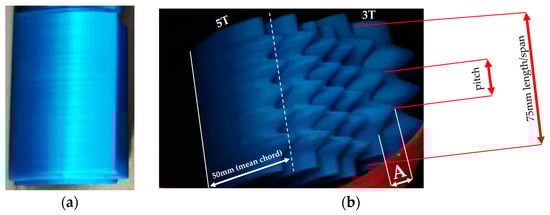
Figure 1.
Serration parameters: (a) baseline; (b) LE serrations.
As in [36], the experimental setup was coupled to a 9800 Pa, 7.5 kW centrifugal fan (SODECA CA-172-2T-10 IE3, Spain) via a corrugated tube (315 mm in diameter) and placed in the anechoic chamber (1200 m3, 15 × 10 × 8 m) designed and executed according to ISO3745 [42] requirements, with a wall absorption coefficient of 99%, in 150–20,000 Hz frequency range. To enable accurate acoustic field measurements, a microphone array was used (Figure 2), similar to those currently employed in advanced research facilities [14,43,44]. The array was implemented using a circular sector (Figure 3), onto which 13 GRAS 40 AE microphones were mounted—arranged across 180 degrees, with a spacing of 15 degrees connected to two SIRIUS Modular Data Acquisition (DAQ) Systems (8 channels) mounted in series. The entire measurement plane can be rotated around its lateral axis using a housed bearing (AVI-3610) and a locking disc with a pin at the desired angular position, enabling consistent data acquisition across multiple configurations. Windscreens were used on the central microphones (located at 0–15 degrees from the longitudinal axis), which proved useful up to a tilt of 15 degrees from the horizontal plane. The acoustic camera shown in Figure 2 was tested in the vicinity of the blade cascade (above placement), but below 2500 Hz, the noise produced by aerodynamic detachment seemed to dominate.
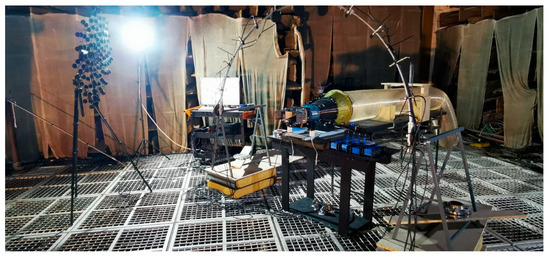
Figure 2.
Schematic of the experimental setup for cascade sector testing.
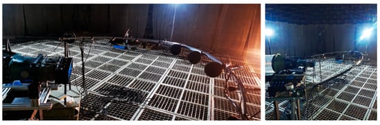
Figure 3.
Microphone positioning along the circular arc.
The tested blades were installed at the nozzle exit, clamped between two plates that set the installation angle within the cascade (Figure 4). Four pairs of plates were used, corresponding to incidence angles of 0°, 5°, 10°, and 15°, respectively. Prior to the main experimental campaign, preliminary recordings were conducted to capture the acoustic spectrum generated by the turbulence-inducing grid, using both a flush-mounted surface microphone and an aerodynamically profiled probe (Figure 5).
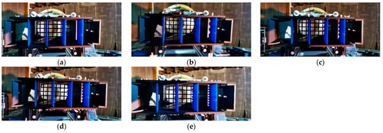
Figure 4.
Blade installation within the cascade: (a) baseline; (b) 3 teeth; (c) 5 teeth; (d) 7 teeth; (e) 9 teeth.
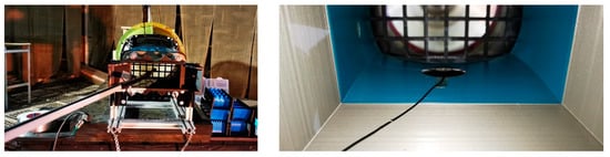
Figure 5.
Microphone placement for turbulence parameter identification (left—aerodynamically profiled microphone, right—surface microphone).
Turbulence parameters—namely the velocity fluctuation intensity and the characteristic length scale of coherent structures—were estimated using an indirect approach based on acoustic measurements acquired downstream of a passive turbulence-generating grid. The recorded pressure signals contain spectral information associated with the turbulent interaction between the flow and the channel walls, allowing for the extraction of relevant turbulence descriptors. The experiments were carried out in a test channel with a cross-sectional area of approximately 125 mm × 75 mm (in the final portion of the setup, where the area remains relatively constant up to the exit), in which a fixed turbulence grid was mounted (the most effective variant identified in the previous report). This grid was used to generate turbulent structures in the flow. The mean flow velocity in the exit section was 50 m/s. Downstream of the grid, two microphones were positioned:
- A surface microphone, mounted 50 mm from the grid and integrated into the channel wall, intended for measuring the pressure signal at the fluid–solid interface;
- An aerodynamically profiled microphone, placed 30 mm further downstream, inserted directly into the flow to capture the noise generated by vortices.
The recorded data were acquired at a sampling frequency of 50 kHz, and the resulting signals were later processed using the Fourier transform to determine the acoustic pressure spectra and the power spectral density (PSD) for each channel. To estimate the turbulence parameters, a semi-empirical model was used, inspired by flow acoustics literature (see [45]: acoustic source theory—dipole, quadrupole; acoustic spectrum derived from the turbulent autocorrelation function, with spectral forms such as fn·e^(−f/fs); and [46]: pressure spectra radiated by convective turbulent structures, typically of Gaussian or low-exponent form depending on source length and frequency). In this model, the pressure spectral density induced by turbulent structures is approximated using the following relation:
where u′ is the root-mean-square (RMS) velocity fluctuation intensity, U is the mean flow velocity, L is the characteristic length scale of the turbulent structures, f0 = U/L is the reference frequency associated with the integral turbulence scale, and B is an empirical constant. The model is constructed based on the experimental observation that the radiated pressure spectrum increases proportionally to f2 at low frequencies and decays exponentially at high frequencies (with a cut-off frequency defined by f0 ≈ U/L).
The model was fitted by matching the theoretical curve to the experimentally obtained spectrum (from the surface microphone signal—similar to [47]), and the parameters u′/U and L were determined by minimizing the mean square error between the estimated and measured spectra.
To characterize the spectral content of the recorded acoustic pressure, a direct method was used to estimate the power spectral density (PSD), based on the discrete Fourier transform applied to successive segments of the signal. This approach is equivalent to Welch’s method [48], but was implemented explicitly for compatibility with processing in GNU Octave. The signal was divided into Hann windows [49] of 2048 samples each, with 50% overlap between windows, ensuring full coverage of the signal and a stable spectral estimate. For each segment, the Fourier transform was applied, and the squared magnitudes of the spectral coefficients were accumulated and averaged. Finally, the result was normalized by the energy of the applied window, in accordance with standard relationships from spectral estimation theory [50,51].
The power spectral density was then converted to an arbitrary logarithmic level, expressed in decibels (relative SPL), using the following relation:
where P(f) represents the estimated mean power at frequency f. The analyzed frequency range was limited to 100 Hz–20 kHz, thus covering the primary acoustically relevant range for flow-induced noise. This analysis was applied to both recorded signals: the wall-pressure signal (surface microphone) and the in-flow pressure signal (profiled microphone), in order to highlight the spectral content differences caused by the microphones’ relative positions with respect to the turbulent structures.
By applying the base-10 logarithm for numerical stability, the model becomes:
This formulation allows the model to be fitted based on the experimentally obtained acoustic pressure spectrum. In the equation above, the term B also incorporates the factor log10(e) resulting from the logarithmic transformation of the original expression. The fitting procedure involves minimizing the squared difference between the measured spectrum (in dB) and the logarithmic model, within a well-defined spectral range. Based on the optimized parameters, the relative turbulence intensity can be deduced using relation (4), which is also implemented explicitly in the autocorrelation function (within the code)
and the characteristic frequency results from the following:
The value of B is not selected arbitrarily, nor does it result directly from an explicit system of equations. Instead, it is obtained by minimizing the difference between the theoretical model (in its logarithmic form) and the measured spectrum, using the so-called curve fitting approach, which can be expressed as follows:
where is a scaling term, L is the characteristic length (obtained through the optimization of the term log10(L)), and B is the constant associated with turbulent energy dissipation. From a physical perspective, the constant B controls the slope of the curve at high frequencies—larger values imply a faster dissipation of turbulent energy. However, B depends on multiple factors (such as viscosity, the spectral limits of the microphone, and flow irregularities) and cannot universally be assumed to be equal to 1.
In this analysis, instead of using the spectrum in logarithmic units such as SPL (sound pressure level, expressed in decibels), the representation was performed directly in terms of the power spectral density (PSD) in physical units, Pa2/Hz. The PSD preserves the linearity of energy distribution across frequencies, thus allowing direct comparison between theoretical models and experimental data, without the arbitrary influence of a logarithmic reference (e.g., 20 µPa). As such, the use of power spectral density offers a more accurate and physically consistent framework for identifying turbulence characteristics from recorded acoustic signals, particularly when aiming to correlate with theoretical models based on energy, rather than on auditory perception.
The spectra recorded by the two microphones are shown in Figure 6. On the raw data, the following operations were applied: segmentation into Hann windows with 50% overlap, FFT applied to each window, spectral energy averaging, normalization of the result using the window energy (as implemented in the code, with a structure similar to the pwelch function in MATLAB), construction of the frequency vector, and representation of the sound pressure level (SPL) distribution.
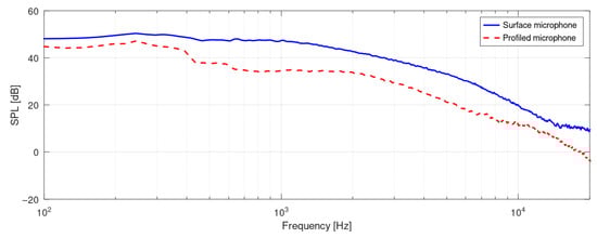
Figure 6.
FFT on raw data—surface microphone/profiled microphone.
The estimation of turbulence parameters based on the measured acoustic signal can be carried out by analyzing the autocorrelation function of the acoustic pressure [51,52,53], recorded near the turbulent source. This approach is based on the assumption that the pressure signal is proportional to the velocity fluctuations within the turbulent flow, and that its autocorrelation reflects the spatial and temporal structure of the vortices.
The normalized autocorrelation function R(τ) of the pressure signal p(t) is defined as follows:
where τ is the time delay, and R(0) is the value at τ = 0, representing the variance of the signal. Two characteristic turbulence parameters can be estimated from this function. The characteristic length of the turbulent structure, L, is given by the following:
where U is the mean flow velocity, and the integral is numerically approximated up to the first significant zero crossing or up to a fixed threshold (e.g., 5–10 ms; 10 ms used on final results). The turbulence intensity u′/U is derived from the energetic relationship between the signal level and the length L [54], according to the simplified model:
where ρ0 and c0 are the air density and the speed of sound, respectively (assumed constant). By applying this method to the signals recorded with the surface and profiled microphones, the turbulent parameters can be compared at two different locations in the flow field, providing additional insight into the evolution and dissipation of the turbulent structure downstream of the generating grid. Regarding the estimation of u′ (velocity fluctuations), several relations can be applied, as summarized in Table 1.

Table 1.
Models for pressure fluctuation.
By comparing the applied methods, the lower values of the turbulence parameters appear more plausible, as the PSD/autocorrelation approaches integrate the acoustic pressure signals within the energy domain and rely on the plane wave relationship (). For more realistic results, one may employ a model that directly links the acoustic spectrum to turbulent flow (advanced models such as Lighthill [55] and Curle [56]), or rely on direct velocity measurements (e.g., LDA [57], PIV [58], or hot-wire anemometry [59]).
From the results, the turbulence intensity u′/U of 73% obtained from the pressure data interpreted as dynamic components is erroneous, since the nature of the raw signal is different (i.e., acoustic pressure). Figure 7 shows that all methods, within the 100 Hz–20 kHz frequency range, place the characteristic length around 5 mm—a value consistent with expectations from previous report analyses.
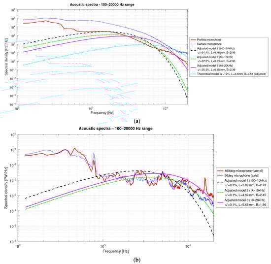
Figure 7.
Overlay of measured and fitted spectra (curve fitting): (a) measurements inside the flow channel; (b) measurements outside the nozzle.
Using either the autocorrelation function or the PSD, the integration of the Suu(f) spectrum can be used to determine the turbulent kinetic energy. The computational process begins from relation (10):
and the relationship between acoustic pressure and velocity can be expressed as follows:
Therefore, for a known Spp(f), the kinetic energy k can be directly computed. It should be noted that the obtained values are local, corresponding to the point where the microphone is positioned, and do not represent the total turbulent energy in the system. This quantity refers only to the longitudinal components (assuming the signal is oriented along a single direction). The spectrum Suu(f) derived from raw pressure assumes plane wave propagation, which may be a reasonable approximation at large distances, but is more questionable near the source.
3. Results
The raw signals recorded by the 12 GRAS 40AE microphones via the Dewesoft acquisition system were processed using FFT and subsequently exported in terms of sound pressure level (SPL). For each spatial position, a single SPL value was obtained and mapped onto the spherical cap shown in Figure 8. These data were then interpolated to produce a much smoother distribution (Figure 9—data samples for baseline and 9 teeth for a brief comparison). The applied methodology is structured as follows: construction of the measurement field (based on known planes and microphone spacing), import of the results for each point, import of the nozzle geometry (simulated as a point cloud), plotting of markers for each point using a color scale corresponding to the SPL value, selection of a single value for the fixed microphones (at 0° and 180°), and surface interpolation on the spherical cap via triangulation (rough method) or v4-type interpolation (specific to MATLAB/Octave, superior to cspline in this case). This processing routine was applied to all available data (various blade–plate combinations for installation angle control), with the results detailed in the following sections.
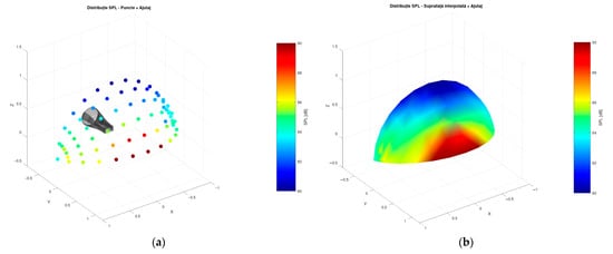
Figure 8.
SPL representation: at measurement points (a) and on the spherical cap ((b), “trisurf” interpolation).
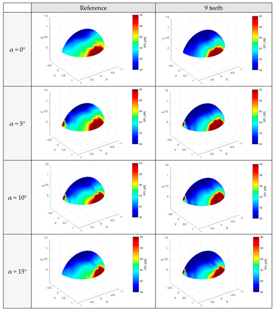
Figure 9.
SPL representation on the spherical cap (“v4” interpolation).
Figure 10 presents the results (as differences in sound pressure level, in dB(Z), RMS) for all combinations of blade geometries and installation angles. Except for the measurement planes at 15° and 30°, where the jet tends to interfere with the microphones surrounding the 6th position (75° and neighboring angles), a global reduction is observed at all positions. The magnitude of this reduction increases as the number of serration peaks (teeth) grows (i.e., as the serration pitch decreases). Notably, configurations with blades having five teeth yield reductions comparable to those with the smallest pitch (nine teeth), indicating significant performance even at intermediate geometries.
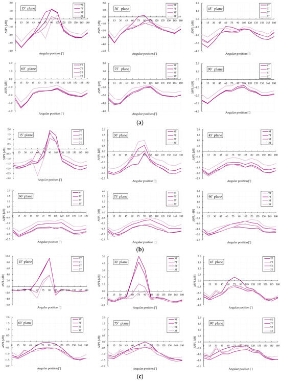
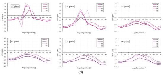
Figure 10.
ΔSPL representation for the tested configurations: (a) α = 0°; (b) α = 5°; (c) α = 10°; (d) α = 15°.
If all microphones are averaged across all positions within the same measurement plane, the result is shown in Figure 11. Two types of averaging are presented here: simple (arithmetic) averaging and logarithmic averaging, the latter being commonly used when differences between microphones exceed 3 dB [60]. The logarithmic averaging was performed using the following relation:
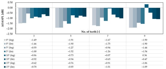
Figure 11.
Global levels (comparison between arithmetic and logarithmic averaging).
For a rapid estimation of serration efficiency along the 1-m radius (covering a 180-degree arc), Table 2 summarizes the noise reduction (in terms of sound pressure level) for all blade and angle combinations, referenced, of course, to their respective baseline configurations.
Table 2.
SPL reduction over the 180-degree arc.
Acoustic beamforming is a spatial signal processing technique applied to data collected from microphone arrays, enabling the localization and quantification of noise sources [61,62]. In turbulent jet noise investigations, beamforming facilitates the reconstruction of spatial sound pressure level (SPL) distributions within a defined observation plane, revealing both the intensity and directional characteristics of the radiated noise field. This approach is particularly valuable for assessing the influence of geometric perturbations, such as blade insertion or modifications to leading-edge profiles, on the acoustic behavior of the jet. In the present study, data were acquired using an array of 13 microphones positioned along a semicircular arc with a radius of 1 m, distributed across several inclined planes ranging from 15° to 90° relative to the XY plane. The jet was produced by a nozzle with a rectangular exit section (75 mm × 125 mm) and operated at a flow velocity of 50 m/s, with a maximum deviation of 15° from the Y-axis, a configuration that directly influences both the orientation of the acoustic radiation and the location of dominant sources. From the frequency perspective, turbulent jet noise is governed by the hydraulic diameter of the nozzle exit and the flow velocity. For the tested nozzle, the hydraulic diameter is estimated as follows:
Using the dimensionless Strouhal number relation, the characteristic frequencies of the noise can be estimated as follows:
This range defines the main acoustic band of interest, where predominant emissions are expected to occur. The frequencies corresponding to the one-third octave bands centered at 1260 Hz, 1600 Hz, 2000 Hz, and 2500 Hz provide relevant coverage within this spectral region.
The beamforming computation involves several successive steps. First, the raw signals from each microphone (recorded separately for each plane) are extracted and windowed (e.g., Hann window, N = 4096) to reduce edge effects. FFT is then applied to compute the spectra:
In the above expression, denotes the signal from microphone i, while w[n] is the applied window. The spatial positions of the microphones, , are known in the 3D coordinate system, and the observation plane is defined in the XY plane (Z = 0), regularly discretized with a fixed spatial step (0.005 m in the code attached in the annexes). For each observation point , the geometric distances to all microphones are computed.
The classical beamforming algorithm relies on the coherent summation of complex spectra, with phase alignment based on geometric delays:
where k = 2πf/c is the wavenumber. The geometric phasing is implemented in the code using steering = exp(−1i * k_val * vecnorm (obs_points – reshape (mic_positions, 1, [], 3), 2, 3)). The SPL level at each observation point is expressed relative to the maximum value within the entire map:
The difference between the constants 10 and 20 in SPL formulas (analytical vs. code implementation) arises from the nature of the processed quantity: for pressure, the correct expression is 20·log10(…), while for power it is 10·log10(…). A methodological challenge stems from the fact that the microphone planes were recorded sequentially, not simultaneously. This prevents the use of coherent 3D beamforming, since the signals cannot be time-synchronized. A valid alternative is the spatial averaging of SPL across individual beamforming maps [63,64,65]:
This strategy provides an estimate of the spatial distribution of the noise field and is applicable even in the absence of temporal coherence between planes. The resulting representations enable the identification of dominant emission directions and the potential effects of geometric perturbations on the acoustic distribution.
The beamforming results presented in Figure 12 are expressed in relative SPL, i.e., decibels referenced to the local maximum within the observation plane, for each analyzed frequency. Although the input signals are calibrated in absolute pressure, the beamforming process does not preserve this physical scale, since the result is obtained through coherent summation of complex pressures—incorporating both constructive and destructive interference—which alters the total amplitude in a phase-dependent manner rather than reflecting energy. Moreover, the propagation model used is one-way, simulating only the forward path from the source to the microphones, and does not enable the inverse estimation of actual pressure at a given spatial point.
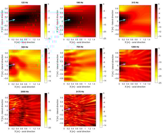
Figure 12.
Beamforming—reference blade (α = 15 degrees).
To obtain absolute SPL at the observation points, an inverse transfer function is required to compensate for the propagation path from the source to the microphones. This can be determined through full numerical modeling using methods such as BEM or FEM, experimental calibration with reference acoustic sources, or through regularized inversion methods such as CLEAN-SC [66] or DAMAS, which solve the inverse beamforming problem based on a propagation model. In the absence of such inverse functions, beamforming maps still provide valuable information regarding the directionality and relative distribution of acoustic energy, making them useful for comparative analysis and dominant source localization.
The transformation of a planar SPL distribution (XY) into a single directivity curve is carried out by aggregating SPL values according to the polar angle associated with each observation point in that plane. This process can be described in simple steps:
- Each observation point in the XY plane has a position (x, y), which can be converted to a polar angle θ with respect to the microphone array center, using
- The angle is adjusted such that 0° corresponds to the vertical upward direction, and angles increase clockwise up to 180°.
- The SPL distribution computed via beamforming yields a value for each (x, y) point, allowing a set of SPL values to be associated with each polar angle θ.
- For each discrete angle (e.g., at 1° intervals), an energy-based averaging of the associated SPL values is performed (e.g., by interpolation and averaging within a narrow angular band, ±0.5°), to obtain a representative sound level for that direction.
- The result is a curve SPL = f(θ), describing how the sound level varies with direction within a given plane.
This curve is referred to as the directivity curve and is used in butterfly or polar plots to synthetically visualize the directional distribution of acoustic energy in a way that enables comparison across planes or frequencies. In the polar representation, each microphone plane is displayed as a curve within a semi-polar coordinate system (0–180°), with SPL values expressed relative to the local maximum.
The representation is designed to highlight the shape and width of the directional lobes, as well as their orientation relative to the jet axis (indicated by an arrow at +15° from the vertical). The curves are interpolated with a 1° angular resolution and scaled such that each plot reflects the local SPL variation within its corresponding plane (Figure 13).
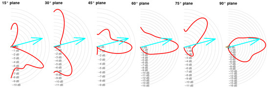
Figure 13.
Directivity—reference blade, 315 Hz (alpha = 15 degrees).
In Figure 14, the 3D representation adds geometric context by reconstructing the shapes of the directional lobes in space, with each plane projected along its corresponding inclination angle (15°–90°). Each curve is relatively scaled and positioned within a common coordinate system, in which the nozzle geometry is also visible. This method enables the assessment of the global orientation of the acoustic source and any asymmetries between planes, complementing the polar analysis with an intuitive depiction of spatial directivity.
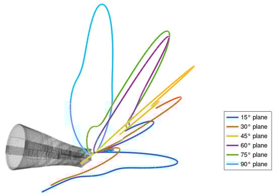
Figure 14.
Directivity on each plane—overlay at nozzle exit.
4. Discussion
Although the overall SPL reduction observed in this study ranges between 2 and 6 dB, these values must be interpreted in the context of the scaled-down experimental setup. The tested blades have a span of 75 mm and a chord of 50 mm, significantly smaller than typical stator blades in turbofan engines, which often exceed 200 mm in span and 100 mm in chord. Furthermore, the jet velocity (50 m/s) is moderate but consistent with experimental studies on low-speed aeroacoustic mechanisms. In logarithmic terms, a 3 dB reduction corresponds to approximately a 50% reduction in acoustic power, while 6 dB represents a 75% reduction. Even the lower bound of 2 dB translates to a power reduction of around 37%, which is non-negligible when integrated over the entire emission surface or scaled to full-size geometries.
Moreover, the spatial distribution of acoustic energy is not uniform. Beamforming and directivity analyses reveal that serrations induce modifications in the shape and orientation of the acoustic lobes. In certain angular sectors, the SPL reduction can exceed the global average, suggesting localized improvements in noise radiation. However, in other regions, energy may be redistributed or even slightly enhanced, depending on the frequency, observer position, and serration configuration. This underlines the importance of full-field spatial analysis in assessing the effectiveness of passive noise control strategies, beyond a single-point or globally averaged metric.
The observed noise reduction associated with increased serration pitch can be physically attributed to a combination of mechanisms. First, the modulation of the leading-edge geometry alters the effective area of interaction with incoming turbulent eddies, redistributing the acoustic sources along the span. Second, serrations introduce spanwise pressure phase differences, which promote destructive interference in the radiated field. This spatial decorrelation effect is more pronounced at higher frequencies and with increased tooth number and amplitude. These phenomena are consistent with findings from previous studies on leading-edge serration aerodynamics and blade aeroacoustics (e.g., references such as [17,19,29,32,33,38,39]). One aspect worth mentioning is that the sources previously listed barely address the cascade effect, as reflections and destructive interference may also play a role in this overall mechanism. Although the present study is primarily experimental, the trends observed suggest the potential to develop semi-empirical or analytical models linking serration parameters—such as pitch (number of teeth) and amplitude (chordwise depth)—to the spectral and spatial characteristics of the radiated noise. As shown in this work, increasing the serration count leads to progressively “smoother” interaction between the incoming turbulence and the blade surface, and to measurable broadband attenuation. Future efforts will focus on quantifying this relationship by extending current analytical formulations for serrated leading edges and integrating turbulence statistics obtained from autocorrelation-based methods.
Although detailed theoretical validation is beyond the scope of this study, it is worth noting that existing predictive models for leading-edge serrations are typically restricted to simplified two-dimensional assumptions or rely on specialized numerical codes, such as Lattice-Boltzmann Methods, which are not readily accessible. Moreover, full 3D comparisons require complex turbulence-resolving simulations, which present challenges in terms of grid sensitivity and frequency bandwidth coverage. As such, the experimental beamforming results presented here—while qualitative in nature—offer a valuable benchmark for future high-fidelity modeling efforts. The observed directional trends and frequency-dependent attenuation patterns can serve as reference targets for validating numerical models under similar inflow and geometrical conditions.
The combined analysis of spatial distribution (Figure 12), directivity (Figure 13), and integrated ΔOASPL values (bar chart—Figure 11) reveals the significant influence of serrations on trailing-edge noise emission. Quantitatively, a consistent SPL reduction is observed across all serrated configurations, with the 5-tooth geometry at 0° installation yielding the most notable attenuation—up to −1.9 dB in both logarithmic and linear integration methods. However, at higher angles of attack (α = 15°) and for configurations with an increased number of teeth (e.g., nine teeth), the noise reduction effect becomes less consistent and even counterproductive in certain cases (e.g., +0.34 dB at 10°, log-integrated), indicating a possible loss of aerodynamic efficiency due to increased flow separation or serration saturation.
From a qualitative perspective, the directivity patterns at 315 Hz (Figure 13) show a clear reshaping of the acoustic lobes in inclined planes, with a redistribution of energy toward wider angles—suggesting enhanced acoustic scattering. This trend is further supported by the beamforming maps (Figure 12), where for intermediate frequencies (e.g., 794–1260 Hz), the dominant source regions appear more diffuse and shifted downstream. This behavior implies reduced coherence of the noise-generating structures and stronger interaction between convective vortices and the serrated trailing edge.
From a dimensional standpoint, these results support the hypothesis that the noise-mitigation performance of serrations is governed by the ratio between the serration geometry and the local turbulence correlation length. Configurations with 5 and 7 teeth appear to strike an optimal balance between diffraction and decoherence, while excessive serration count (9 teeth) or high angles of attack tend to degrade the acoustic performance.
The current calculations are preliminary, with the implemented code validated on several cases (reference and select serrated geometries), using either raw signals or signals processed via FFT to extract global SPL values. A future analysis will address the full dataset to capture clearer trends between noise reduction and the introduced design solution, potentially enabling parametric relationships using standard methods such as regression analysis.
5. Conclusions
This study investigated the potential of leading-edge serrations to reduce noise generated by the interaction between a turbulent jet—representative of upstream rotor wakes—and downstream stator blades. Several geometries were proposed, physically manufactured via 3D printing, and tested on a dedicated experimental rig developed within the facilities of the COMOTI Acoustics Department in Măgurele. The leading-edge serration pitch was varied from 0 (reference blades) to 9 so that specific behaviors related to significant frequencies, directional reductions, or overall efficiency could be correlated with the turbulence-to-serration pitch ratio.
To identify turbulence parameters, signal processing techniques were also applied (based on measurements acquired in this study using either a flush-mounted or profiled microphone). The autocorrelation-based parameters enabled estimation of the characteristic eddy length. A dedicated computational code was developed for this purpose and used to plot the relevant parameters.
The test matrix included five serration configurations and four installation angles, with acoustic data recorded at 13 microphone positions across six inclined planes. Post-processed results revealed consistent reductions in sound pressure levels across the measured hemisphere, reaching up to 2 dB globally. These were further extrapolated to reconstruct the full spatial distribution of acoustic energy. Beamforming and polar directivity analyses enabled the identification of dominant radiation lobes and provided insight into the directional influence of serration geometry.
As an outcome of this analysis, new design insights may emerge, including the use of trailing-edge serrations on the upstream blade and leading-edge serrations on the downstream blade or configurations combining serrations on both edges.
Author Contributions
Conceptualization, A.-G.T., D.-E.C., M.D., G.C., and C.L.; methodology, A.-G.T., M.D., and L.C.; software, A.-G.T., M.D., and L.C.; validation, A.-G.T., M.D., and G.C.; formal analysis, A.-G.T., D.-E.C., and C.L.; investigation, A.-G.T. and G.C.; resources, A.-G.T., M.D., and L.C.; data curation, A.-G.T. and G.C.; writing—original draft preparation, A.-G.T.; writing—review and editing, A.-G.T., D.-E.C., M.D., G.C., and C.L.; visualization, A.-G.T.; supervision, D.-E.C., M.D., G.C. and C.L. All authors have read and agreed to the published version of the manuscript.
Funding
This research received no external funding.
Institutional Review Board Statement
Not applicable.
Informed Consent Statement
Not applicable.
Data Availability Statement
The original contributions presented in this study are included in the article; further inquiries can be directed to the corresponding author.
Acknowledgments
The data presented and analysed in this report were obtained with the help of INCDT COMOTI’s Research and Experiments Center in the field of Acoustic and Vibrations (ACUVIB) staff and facility, and the work was carried out with the anechoic chamber and measurement equipment.
Conflicts of Interest
The authors declare no conflicts of interest.
Nomenclature
The following abbreviations are used in this manuscript:
| c | airfoil chord [mm] |
| cmed | mean chord [mm] |
| speed of sound [m/s] | |
| f | frequency [mm] |
| f0 | cut-off frequency [Hz] |
| acoustic intensity [W/m2] | |
| turbulent kinetic energy [m2/s2] | |
| acoustic pressure (RMS values) | |
| s | blade length [mm] |
| velocity fluctuation [mm/s] | |
| signal amplitude/scaling factor | |
| Dh | hydraulic diameter [mm] |
| cumulative acoustic energy [W] | |
| ΔOASPL | global sound pressure level reduction [dB(Z)] |
| L | characteristic length of turbulent structures [mm] |
| Lp, SPL | sound pressure level [dB(Z)] |
| N | number of computational points [-] |
| P | acoustic power [W/m3] |
| autocorrelation function | |
| , PSD | pressure spectral density [Pa2/Hz] |
| , U | (mean) jet velocity [m/s] |
| α | blade installation angle in array [°] |
| dΩeff | solid angle [sr] |
| λ | serration pitch [mm] |
| density [kg/m3] | |
| observer angle [ad] | |
| calculation point position [m] | |
| τ | time delay [ms] |
References
- Shenoy, D.V.; Gojon, R.; Jardin, T.; Jacob, M.C. Aerodynamic and acoustic study of a small scale lightly loaded hovering rotor using large eddy simulation. Aerosp. Sci. Technol. 2024, 150, 109219. [Google Scholar] [CrossRef]
- Leishman, J.G. Acoustics of Flight Vehicles. Introduction to Aerospace Flight Vehicles. Available online: https://eaglepubs.erau.edu/introductiontoaerospaceflightvehicles/chapter/noise-of-flight-vehicles/ (accessed on 1 July 2025).
- Xie, J.; Zhu, L.; Lee, H.M. Aircraft Noise Reduction Strategies and Analysis of the Effects. Int. J. Environ. Res. Public Health 2023, 20, 1352. [Google Scholar] [CrossRef]
- Le Garrec, T.; Polacsek, C.; Chelius, A.; Daroukh, M.; François, B. Tone Noise Predictions of a Full-Scale UHBR Engine at Approach Condition with Inflow Distortion Effects. In Proceedings of the 25th AIAA/CEAS Aeroacoustics Conference, Delft, The Netherlands, 20–23 May 2019. [Google Scholar]
- Moreau, S. Turbomachinery Noise Predictions: Present and Future. Acoustics 2019, 1, 92–116. [Google Scholar] [CrossRef]
- Yang, X.; Liu, T.; Jia, W. Research on the Aerodynamic–Propulsion Coupling Characteristics of a Distributed Propulsion System. Appl. Sci. 2025, 15, 3536. [Google Scholar] [CrossRef]
- Salehian, S.; Mankbadi, R. Jet Noise in Airframe Integration and Shielding. Appl. Sci. 2020, 10, 511. [Google Scholar] [CrossRef]
- Dombrovschi, M.; Deaconu, M.; Cristea, L.; Frigioescu, T.F.; Cican, G.; Badea, G.-P.; Totu, A.-G. Acoustic Analysis of a Hybrid Propulsion System for Drone Applications. Acoustics 2024, 6, 698–712. [Google Scholar] [CrossRef]
- Moreau, S.; Roger, M. Turbomachinery Noise Review. Int. J. Turbomach. Propuls. Power 2024, 9, 11. [Google Scholar] [CrossRef]
- Palma, G.; Burghignoli, L.; Centracchio, F.; Iemma, U. Innovative Acoustic Treatments of Nacelle Intakes Based on Optimised Metamaterials. Aerospace 2021, 8, 296. [Google Scholar] [CrossRef]
- Kenchappa, B.; Shivakumar, K. Evaluation of a Microporous Acoustic Liner Using Advanced Noise Control Fan Engine. Appl. Sci. 2025, 15, 4734. [Google Scholar] [CrossRef]
- dos Santos, F.L.; Venner, C.H.; de Santana, L.D. Tripping Device Effects on the Turbulent Boundary Layer Development. In Proceedings of the AIAA AVIATION 2022 Forum, Chicago, IL, USA & Virtual, 27 June–1 July 2022. [Google Scholar] [CrossRef]
- Amirsalari, B.; Rocha, J. Recent Advances in Airfoil Self-Noise Passive Reduction. Aerospace 2023, 10, 791. [Google Scholar] [CrossRef]
- Geyer, T.F.; Wasala, S.H.; Sarradj, E. Experimental Study of Airfoil Leading Edge Combs for Turbulence Interaction Noise Reduction. Acoustics 2020, 2, 207–223. [Google Scholar] [CrossRef]
- Sesalim, D.; Naser, J. Effects of an Owl Airfoil on the Aeroacoustics of a Small Wind Turbine. Energies 2024, 17, 2254. [Google Scholar] [CrossRef]
- Tian, C.; Liu, X.; Wang, L.; Li, Y.; Wu, Y. Analytical Solution and Analysis of Aerodynamic Noise Induced by the Turbulent Flow Interaction of a Plate with Double-Wavelength Bionic Serration Leading Edges. Biomimetics 2025, 10, 193. [Google Scholar] [CrossRef]
- Gruber, M. Airfoil Noise Reduction by Edge Treatments. Ph.D. Thesis, University of Southampton, Southampton, UK, 2012. [Google Scholar]
- Agrawal, B.R. Modeling Fan Broadband Noise from Jet Engines and Rod-Airfoil Benchmark Case for Broadband Noise Prediction. Master’s Thesis, Iowa State University, Ames, IA, USA, 2015. Available online: https://lib.dr.iastate.edu/etd/14326 (accessed on 1 July 2025).
- Narayanan, S.; Joseph, P.; Haeri, S.; Kim, J.W.; Chaitanya, P.; Polacsek, C. Noise Reduction Studies from the Leading Edge of Serrated Flat Plates. In Proceedings of the 20th AIAA/CEAS Aeroacoustics Conference, Atlanta, GA, USA, 16–20 June 2014. [Google Scholar] [CrossRef]
- Jiang, M.; Li, X.-D.; Zhou, J.-J. Experimental and numerical investigation on sound generation from airfoil-flow interaction. Appl. Math. Mech. 2011, 32, 765–776. [Google Scholar] [CrossRef]
- Teruna, C.; Avallone, F.; Casalino, D.; Ragni, D. Numerical investigation of leading edge noise reduction on a rod-airfoil configuration using porous materials and serrations. J. Sound Vib. 2021, 494, 115880. [Google Scholar] [CrossRef]
- Liu, L.; Zhang, L.; Wu, B.; Chen, B. Numerical and Experimental Studies on Grid Generated Turbulence în Wind Tunnel. J. Eng. Sci. Technol. Rev. 2017, 10, 159–169. [Google Scholar] [CrossRef]
- Lau, A.S.H.; Haeri, S.; Kim, J.W. The effect of wavy leading edges on aerofoil–gust interacțion noise. J. Sound Vib. 2013, 332, 6234–6253. [Google Scholar] [CrossRef]
- Polacsek, C.; Barrier, R.; Kohlhaas, M.; Carolus, T.; Kausche, P.; Moreau, A.; Kennepohl, F. Turbofan Interaction Noise Reduction Using Trailing Edge Blowing: Numerical Design and Assessment and Comparison with Experiments.V2. Aerospacelab 2014, 7, 1–9. [Google Scholar] [CrossRef]
- Dan, R. The International Civil Aviation Organization’s CAEP/13 Aircraft Noise Standards. 2025. Available online: https://theicct.org/wp-content/uploads/2025/05/ID-358-%E2%80%93-Noise-standard_ICAO_final.pdf (accessed on 1 July 2025).
- EASA Certification Noise Levels. n.d. EASA. Available online: https://www.easa.europa.eu/en/domains/environment/easa-certification-noise-levels (accessed on 1 July 2025).
- Oleksandr, Z. Balanced Approach to Aircraft Noise Management. In Aviation Noise Impact Management; Springer: Cham, Switzerland, 2022. [Google Scholar] [CrossRef]
- ICAO ENVIRONMENTAL REPORT. n.d. Available online: https://www2023.icao.int/environmental-protection/Documents/EnvironmentalReports/2016/ENVReport2016_pg38-41.pdf (accessed on 1 July 2025).
- Chaitanya, P.; Joseph, P.; Chong, T.P.; Priddin, M.; Ayton, L. On the Noise Reduction Mechanisms of Porous Aerofoil Leading Edges. J. Sound Vib. 2020, 485, 115574. [Google Scholar] [CrossRef]
- Zamponi, R.; Satcunanathan, S.; Moreau, S.; Ragni, D.; Meinke, M.; Schröder, W.; Schram, C. On the Role of Turbulence Distortion on Leading-Edge Noise Reduction by Means of Porosity. J. Sound Vib. 2020, 485, 115561. [Google Scholar] [CrossRef]
- Alexander, P.; Schröffer, A. AST 2017 SIMULATION of HELMHOLTZ RESONANCE EFFECTS in AIRCRAFT ECS. Available online: https://elib.dlr.de/111334/1/AST2017_Paper117_Pollok.pdf (accessed on 4 June 2025).
- Biedermann, T.M.; Chong, T.P.; Kameier, F.; Paschereit, C.O. Statistical–Empirical Modeling of Airfoil Noise Subjected to Leading-Edge Serrations. AIAA J. 2017, 55, 3128–3142. [Google Scholar] [CrossRef]
- Lacagnina, G.; Chaitanya, P.; Kim, J.-H.; Berk, T.; Joseph, P.; Choi, K.-S.; Ganapathisubramani, B.; Hasheminejad, S.M.; Chong, T.P.; Stalnov, O.; et al. Leading edge serrations for the reduction of aerofoil self noise at low angle of attack, pre-stall and post-stall conditions. Int. J. Aeroacoustics 2020, 20, 130–156. [Google Scholar] [CrossRef]
- Zhang, C.; Cheng, W.; Du, T.; Sun, X.; Shen, C.; Chen, Z.; Liang, D. Experimental and Numerical Study on Noise Reduction of Airfoil with the Bioinspired Ridge-like Structure. Appl. Acoust. 2022, 203, 109190. [Google Scholar] [CrossRef]
- Lu, Y.; Li, Z.; Chang, X.; Chuang, Z.; Xing, J. An Aerodynamic Optimization Design Study on the Bio-Inspired Airfoil with Leading-Edge Tubercles. Eng. Appl. Comput. Fluid Mech. 2021, 15, 292–312. [Google Scholar] [CrossRef]
- Totu, A.-G.; Cican, G.; Crunțeanu, D.-E. Serrations as a Passive Solution for Turbomachinery Noise Reduction. Aerospace 2024, 11, 292. [Google Scholar] [CrossRef]
- Wang, Y.; Zhao, K.; Lu, X.-Y.; Song, Y.-B.; Bennett, G.J. Bio-Inspired Aerodynamic Noise Control: A Bibliographic Review. Appl. Sci. 2019, 9, 2224. [Google Scholar] [CrossRef]
- Polacsek, C.; Cader, A.; Buszyk, M.; Barrier, R.; Gea-Aguilera, F.; Posson, H. Aeroacoustic Design and Broadband Noise Predictions of a Fan Stage with Serrated Outlet Guide Vanes. Phys. Fluids 2020, 32, 107107. [Google Scholar] [CrossRef]
- Ye, X.; Zheng, N.; Zhang, R.; Li, C. Effect of serrated trailing-edge blades on aerodynamic noise of an axial fan. J. Mech. Sci. Technol. 2022, 36, 2937–2948. [Google Scholar] [CrossRef]
- Craig, M.E. Trailing-Edge Blowing of Model Fan Blades for Wake Management. Ph.D. Dissertation, Virginia Tech, Blacksburg, VA, USA, 2005. [Google Scholar]
- Totu, A.-G.; Deaconu, M.; Cristea, L.; Bogoi, A.; Crunțeanu, D.-E.; Cican, G. Experimental Analysis of Acoustic Spectra for Leading/Trailing-Edge Serrated Blades in Cascade Configuration. Processes 2024, 12, 2613. [Google Scholar] [CrossRef]
- ISO 3745:2012; Acoustics—Determination of Sound Power Levels and Sound Energy Levels of Noise Sources Using Sound Pressure—Precision Methods for Anechoic Rooms and Hemi-Anechoic Rooms. ISO: Geneva, Switzerland, 2012. Available online: https://www.iso.org/standard/45362.html (accessed on 2 July 2025).
- Yu, X.; Zhou, J.; Li, Y. Noise Control in Tandem Airfoil Configurations Using Leading-Edge Serrations on the Front Airfoil. Exp. Fluids 2025, 66, 103. [Google Scholar] [CrossRef]
- Piccolo, A.; Zamponi, R.; Avallone, F.; Ragni, D. Turbulence Distortion and Leading-Edge Noise. Phys. Fluids 2024, 36, 125183. [Google Scholar] [CrossRef]
- Goldstein, M.E. Aeroacoustics; McGraw-Hill International: Columbus, OH, USA, 1976; Available online: https://archive.org/details/Aeroacoustics/page/52/mode/2up (accessed on 1 July 2025).
- Tam, C.K.W. Computational Aeroacoustics-Issues and Methods. AIAA J. 1995, 33, 1788–1796. Available online: https://www.studocu.com/gr/document/eoniko-metsobio-polytexneio/aeroakoystikh/computational-aeroacoustics-issues-and-methods-tam1995/30207542 (accessed on 1 July 2025). [CrossRef]
- Cawser, S. Acoustic Measurements in Airflow, AECOM. Available online: https://www.ioa.org.uk/sites/default/files/Acoustic%20measurements%20in%20airflow%20Mar_Apr%202019.pdf (accessed on 1 July 2025).
- Welch’s Power Spectral Density Estimate—MATLAB Pwelch. n.d. www.mathworks.com. Available online: https://www.mathworks.com/help/signal/ref/pwelch.html (accessed on 1 July 2025).
- Siemens PLM. 2019. Siemens.com. 2019. Available online: https://community.sw.siemens.com/s/article/window-types-hanning-flattop-uniform-tukey-and-exponential (accessed on 1 July 2025).
- Fourier Analysis and Power Spectral Density 4.1 Fourier Series and Transforms. n.d. Available online: https://www.fccdecastro.com.br/pdf/FAPSD.pdf (accessed on 4 June 2025).
- Stanley, C. ECE 302: Lecture 10.6 Power Spectral Density. Available online: https://engineering.purdue.edu/ChanGroup/ECE302/files/Slide_10_06.pdf (accessed on 4 June 2025).
- Chapter 7 Basic Turbulence. n.d. Available online: https://www.astronomy.ohio-state.edu/ryden.1/ast825/ch7.pdf (accessed on 1 July 2025).
- Agrawal, B.R.; Sharma, A. Aerodynamic Noise Prediction for a Rod-Airfoil Configuration Using Large Eddy Simulations. In Proceedings of the 28th AIAA/CEAS Aeroacoustics 2022 Conference, Atlanta, GA, USA, 16–20 June 2014. [Google Scholar] [CrossRef]
- Michael, C. Turbulence and Noise. Available online: https://people.bath.ac.uk/ensmjc/Notes/tnoise.pdf (accessed on 1 July 2025).
- Lighthill, M.J. On Sound Generated Aerodynamically. I. General Theory. Proc. R. Soc. Lond. Ser. A Math. Phys. Sci. 1952, 211, 564–587. Available online: https://www.jstor.org/stable/98943 (accessed on 1 July 2025).
- Curle The Influence of Solid Boundaries upon Aerodynamic Sound. Proc. R. Soc. Lond. Ser. A Math. Phys. Sci. 1955, 231, 505–514. Available online: http://www.jstor.org/stable/99804 (accessed on 1 July 2025).
- Lau, Y.L.; So, R.M.C.; Leung, R.C.K. Flow-Induced Vibration of Elastic Slender Structures in a Cylinder Wake. J. Fluids Struct. 2004, 19, 1061–1083. [Google Scholar] [CrossRef]
- Troolin, D.R.; Longmire, E.K.; Lai, W.T. Time Resolved PIV Analysis of Flow over a NACA 0015 Airfoil with Gurney Flap. Exp. Fluids 2006, 41, 241–254. [Google Scholar] [CrossRef]
- Fischer, A. Hot Wire Anemometer Turbulence Measurements in the Wind Tunnel of LM Wind Power; Wind Energy Department, Technical University of Denmark: Lyngby, Denmark, 2012; DTU Wind Energy E No. 0006. [Google Scholar]
- Understanding the 3dB Rule—Pulsar Instruments. n.d. Available online: https://pulsarinstruments.com/news/understanding-3db-rule/ (accessed on 1 July 2025).
- Kaneko, S.; Ozawa, Y.; Nakai, K.; Saito, Y.; Nonomura, T.; Asai, K.; Ura, H. Data-Driven Sparse Sampling for Reconstruction of Acoustic-Wave Characteristics Used in Aeroacoustic Beamforming. Appl. Sci. 2021, 11, 4216. [Google Scholar] [CrossRef]
- Sarradj, E. Three-dimensional acoustic source mapping with different beamforming steering vector formulations. Adv. Acoust. Vib. 2012, 2012, 292695. [Google Scholar] [CrossRef]
- Castellini, P.; Martarelli, M. Acoustic Beamforming: Analysis of Uncertainty and Metrological Performances. Mech. Syst. Signal Process. 2007, 22, 672–692. [Google Scholar] [CrossRef]
- Silva, I. Mathematics of Beam Forming-Ikaro Silva-Medium. Medium. 2023. Available online: https://medium.com/@ikarosilva/mathematics-of-beam-forming-a518e59542ad (accessed on 2 July 2025).
- Van Veen, B.; Buckley, K.M. Beamforming Techniques for Spatial Filtering; CRC Press LLC: Boca Raton, FL, USA, 2000. Available online: https://dsp-book.narod.ru/DSPMW/61.PDF (accessed on 1 July 2025).
- Chu, Z.; Zhao, S.; Yang, Y.; Yang, Y. Deconvolution Using CLEAN-SC for Acoustic Source Identification with Spherical Microphone Arrays. J. Sound Vib. 2018, 440, 161–173. [Google Scholar] [CrossRef]


Disclaimer/Publisher’s Note: The statements, opinions and data contained in all publications are solely those of the individual author(s) and contributor(s) and not of MDPI and/or the editor(s). MDPI and/or the editor(s) disclaim responsibility for any injury to people or property resulting from any ideas, methods, instructions or products referred to in the content. |
© 2025 by the authors. Licensee MDPI, Basel, Switzerland. This article is an open access article distributed under the terms and conditions of the Creative Commons Attribution (CC BY) license (https://creativecommons.org/licenses/by/4.0/).