Article

Long Short-Term Memory Mixture Density Network for Remaining Useful Life Prediction of IGBTs

Centro de Automática y Robótica, CSIC-Universidad Politécnica de Madrid, 28500 Madrid, Spain
*
Author to whom correspondence should be addressed.
Technologies 2025, 13(8), 321; https://doi.org/10.3390/technologies13080321
Submission received: 7 June 2025 / Revised: 4 July 2025 / Accepted: 25 July 2025 / Published: 30 July 2025
(This article belongs to the Section Information and Communication Technologies)

Abstract

A reliable prediction of the remaining useful life of critical electronic components, such as insulated gate bipolar transistors, is necessary for preventing failures in many industrial applications. Recently, diverse machine-learning techniques have been used for this task. However, they are generally focused on capturing the temporal dependencies or on representing the probabilistic nature of the degradation of the device. This work proposes a neural network architecture that combines long short-term memory and mixture density networks to address both targets simultaneously when modeling the remaining useful life. The proposed model was trained and evaluated using a real dataset of insulated gate bipolar transistors, demonstrating a high capacity for predicting the remaining useful life of the validation devices. The proposed model outperformed the other algorithms considered in the study in terms of root mean squared error and coefficient of determination. In general terms, an average reduction of at least 18% of the root mean squared error was obtained when compared with the second-best model among those considered in this work, but in some specific cases, the root mean squared error during the prediction of remaining useful life decreased up to 21%. In addition to the high performance obtained, the characteristics of the network output also facilitated the creation of confidence intervals, which are more informative than solely exact values for decision-making.

1. Introduction

Power electronics devices and systems are at the core of many modern applications, and their relevance is expected to continue to grow in the future, with an estimated market size of USD 97.2 billion by 2030 [1]. One key challenge for the next generation of power electronics designs is to increase the efficiency of devices and systems. In situ prognostics and health management are key features to meet future reliability, sustainability, and lifecycle management requirements in the context of Industry 4.0 [2].
Insulated gate bipolar transistors (IGBTs) are key components in the field of power electronics. They are used in a wide range of applications, including motor drives, renewable energy systems, and industrial automation. The performance and health of IGBTs have a significant impact on an electronic system’s reliability and operational efficiency. The failure of an IGBT can lead to major disruptions, costly downtimes, and in extreme cases, catastrophic consequences. As a result, the accurate estimation of the remaining useful life (RUL) of IGBTs has become a crucial task in power electronics, enabling condition-based monitoring, predictive maintenance, and real-time dynamic operational adjustments [3]. Predicting IGBTs’ RUL is also of utmost importance from an economic viewpoint to schedule maintenance or replacement before the failure [4]. Therefore, any improvement in RUL estimation performance using efficient and reliable models represents one step forward in the progress beyond the state-of-the-art.
In recent years, machine-learning and deep-learning techniques have been receiving a significant amount of interest due to their capacity to identify complex temporal patterns and make precise predictions based on previous historical data [5,6,7,8]. Specifically, long short-term memory (LSTM) networks have proven to be an effective tool for sequential data processing, especially when used for time-series forecasting applications [9,10]. LSTM’s ability to capture long-term dependencies and learn from sequential data makes this type of network a natural candidate for RUL prediction [11,12]. However, certain aspects of RUL prediction, such as the inherent uncertainty present in some applications caused by environmental and functional disturbances, can be challenging for LSTM models to adequately represent on their own [13,14]. Consequently, the exploitation and assimilation of this approach by Industry 4.0 stakeholders have been limited due to the lack of quantification of the predictions’ uncertainties [15].
Alternatively, probabilistic approaches to RUL provide a measure of the uncertainty in the predictions, which can be critical for decision-making in maintenance planning [16,17]. Among the machine-learning methods for dealing with the uncertainty of predictions is the mixture density network (MDN), which offers a versatile framework for representing complex probability distributions. MDNs can explicitly capture the uncertainty present in an application by representing the data distribution as a combination of several probability distributions [18]. This capability makes MDNs well-suited for handling scenarios in which the RUL is inherently uncertain and varies across different conditions and contexts. However, since this approach is not inherently specialized in processing sequential data, it may fail to capture the temporal dependencies during the aging of the device.
In this study, a novel approach to RUL prediction of IGBTs by integrating into a single neural network architecture both LSTM and MDNs is proposed. This neural network architecture will be referred to as LSTM-MDN from now on in this paper. The goal of this approach is to successfully represent the probabilistic nature of RUL prediction using MDN, while also taking advantage of the sequence-modeling capabilities of LSTM for capturing long-term dependencies in data, resulting, ultimately, in more reliable and accurate RUL forecasts. This simple yet effective neural network architecture aims to offer more adequate predictions for decision-making in industrial setups by quantifying the uncertainty of the estimated RUL.
The rest of this paper is structured as follows. Section 2 presents a review of related works in LSTM and MDN for RUL prediction. Next, Section 3 presents the architecture and components of the proposed LSTM-MDN, as well as the experimental setup. In Section 4, the results of the experiments are presented. Finally, in Section 5, the contributions of this study are summarized, and future research directions are presented.

2. Related Work

Occasionally, IGBTs can suddenly fail without any prior warning signs being perceived due to catastrophic events (e.g., overvoltage, short circuits). However, this is not the most common situation in aging-related failures. Normally, device failures are preceded by precursory symptoms indicative of underlying degradation mechanisms, such as bond wire lift-off, solder fatigue, and die attach delamination. These degradation processes typically manifest through changes in electrical or thermal parameters before ultimate failure occurs. Based on this idea, prior studies involving IGBTs have exploited the LSTM networks’ temporal pattern identification capabilities for estimating the RUL of these devices. Unlike simpler models, LSTM can retain its state over longer time horizons, making it well-suited for capturing slowly evolving degradation trends and subtle pre-failure patterns. This aligns well with the operational behavior of IGBTs in real-world applications, where degradation signals often unfold across hundreds or thousands of cycles.
A study that uses collector–emitter voltage as a failure precursor and LSTM as an RUL estimator has achieved errors of only 7.6%, 6.4%, and 2.5% when using 12%, 35%, and 58% of the IGBT aging data, respectively [19]. In this case, the data used was collected from an aging platform with thermal circuits designed to induce bond wire and solder degradation. The LSTM-based prediction method outperformed two well-established approaches for this goal, namely the Coffin–Manson and exponential fitting models. The LSTM model particularly excelled in the early stages of device aging with limited data.
In a different study, the collector–emitter spike voltage was selected as the aging feature used as input to an LSTM network whose hyperparameters were optimized using the grid search method. Then, this study proposed to pass the output of the LSTM network to a Gaussian naïve Bayes classifier to predict the RUL [20].
Other approaches have explored hybrid neural networks that combine a convolutional neural network (CNN) and LSTM layers for modeling the IGBT gate oxide layer RUL [21]. In this case, the gate leakage current has been selected as the failure precursor rather than the more commonly studied collector-emitter voltage. Additionally, advanced data preprocessing techniques, including gray correlation analysis, Mahalanobis distance, and Kalman filter, have been applied. The proposed CNN-LSTM model achieved a mean absolute error of 0.0216, outperforming standalone CNN, LSTM, support vector regression (SVR), and Gaussian process regression (GPR) models in experiments using the National Aeronautics and Space Administration (NASA) IGBT public dataset.
Recently, a study has included an attention mechanism in a bi-directional LSTM (Bi-LSTM) model and optimized its hyperparameters using the snake optimizer, which helped to calculate the allocation weight of the time series, enhancing the expression ability of the non-linear features of the hidden layer. This approach has yielded encouraging results for the estimation of the IGBTs’ RUL [22].
The understanding of the physical properties involved in the aging process of IGBTs has allowed for the implementation of a physics-informed LSTM network by including proper constraints in the loss function [23]. In this case, the collector–emitter voltage has been used as a precursor signal, and it has been subjected to several preprocessing techniques, including average down-sampling, standardization, and window smoothing. The proposed network has improved the mean squared error by 51.3% and 13.9% compared to baseline recurrent neural network (RNN) and LSTM models, respectively.
Additionally, LSTM has proven to be an effective method for RUL prediction in other application fields, such as ring oscillator failure [24], bearing fault detection [25], and degradation of aircraft engines [26], among others.
In the case of MDNs, no studies have been found in the scientific literature related to the prediction of an IGBT’s RUL. Furthermore, there are very few works where this type of network has been applied to RUL prediction in different research areas without combining it with other approaches. One of them has explored the use of MDNs for forecasting the RUL of lithium-ion batteries [27]. For this, a set of features, including the differential capacity–voltage and temperature–voltage, has been proposed. This method was validated with three datasets, which contain batteries of different chemistries and operated under different conditions, demonstrating a high generalization capability. Additionally, the model was capable of providing appropriate conditional probability distributions of the target. In a different research area, a novel method based on MDNs has been used for predicting the degradation of machine tools [28]. Specifically, an adversarial-learning approach has been proposed to deal with domain-invariant features, while the probabilistic output produced by the MDN helped reduce the influence of noise and abnormalities caused by sensor precision degradation.
Despite the potential benefits of combining LSTM and MDNs, to the best of the authors’ knowledge, this approach has never been used before for IGBT RUL prediction. Moreover, this approach remains mainly unexplored in the scientific literature, with only a small number of studies in other fields. For instance, a recurrent network that incorporates deep three-dimensional convolutional features, LSTM, and MDN layers has been proposed for modeling spatiotemporal visual attention, allowing the generation of saliency maps for videos. This approach enabled state-of-the-art action classification on two datasets [29]. A deep bidirectional LSTM and MDN model has been used for predicting basketball trajectory, outperforming other models in terms of convergence speed and error when tested on real data. The hyperparameters of this model were optimized using the Hyperopt library, enabling the development of a highly accurate hit-or-miss classifier [30]. Another study has explored the combination of LSTM and MDN for wind power prediction, resulting in a high-performance network capable of providing accurate estimations up to 48 h in advance [31]. This approach has also been used for demand forecasting in electronic retail, allowing simultaneous modeling of associative factors, time-series trends, and the variance in the demand. One of the factors that enabled the accomplishment of these results was the use of feature embeddings to preprocess the input data [32]. A neural network architecture combining LSTM and MDN has been developed for traffic forecasting in complex agent-to-agent and agent-to-scene interactions, providing multimodal distributions for trajectory forecasting [33]. A second study has applied this approach to traffic flow prediction, outperforming a classic LSTM network and an autoregressive integrated moving average (ARIMA) model, predicting traffic flow indices up to 30 min in advance. This study has proposed the use of multi-step sequences for both input and output data [34]. A different study proposed a model that uses a feedforward layer for dimensionality reduction, several LSTM layers to capture temporal patterns, and an MDN layer for emulating trend shifts and variability. This model has been evaluated in three energy market datasets, obtaining remarkable results for high variability time series [35].
After reviewing the existing literature, it is evident that current approaches for RUL prediction of IGBTs often address either the sequential dependency of sensor signals or the inherent uncertainty in RUL estimation, but rarely both in a unified approach. Traditional data-driven models primarily focus on learning direct mappings between the input features and RUL, disregarding the temporal nature of the aging process. Recurrent neural network architectures, on the other hand, are specialized in capturing long-term dependencies in sequential data, making them effective for modeling the progressive aging of IGBTs over time. However, they are trained using deterministic loss functions, which limit their ability to account for the uncertainty in RUL predictions. Combining LSTM and MDN offers a promising approach to address this gap, enabling a model capable of capturing temporal patterns while handling complex probabilistic RUL distributions. This is particularly important in IGBT, where operational and environmental variations can lead to significant uncertainty in failure progression. The LSTM-MND combined approach aims to offer a more comprehensive predictive model, enabling both improved accuracy and uncertainty quantification. The practical significance of this methodology lies in its ability to provide more reliable and interpretable RUL predictions, which are critical for predictive maintenance strategies in power electronics applications. By quantifying uncertainty, the model can support risk-aware decision-making, allowing the optimization of maintenance schedules based on confidence levels rather than relying on deterministic predictions.

3. Materials and Methods

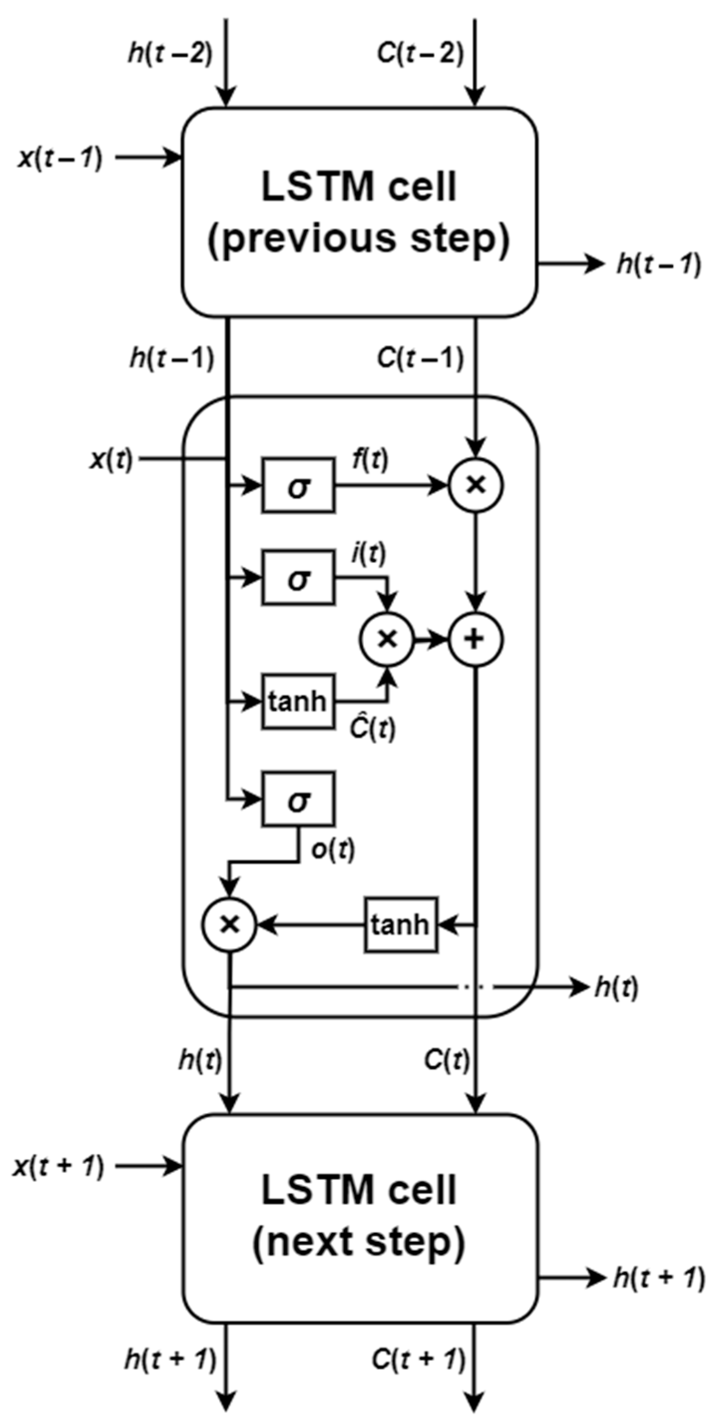
3.1. Network Architecture

The network architecture proposed in this study includes two types of specialized layers. The first one is the LSTM layer, also called the LSTM cell. An LSTM cell contains several key components for determining which information to remember or forget over time. Specifically, LSTM cells implement three gates, namely an input gate ( i ), a forget gate ( f ), and an output gate ( o ), and two state variables: cell state ( C ) and hidden state ( h ). Both state variables are recurrently passed to the cell, which also receives the input data. Additionally, the state variable h represents the output of the cell. Figure 1 shows an unrolled representation over time of an LSTM cell. The values of the components of an LSTM cell are computed using the following equations [36]:
f t = σ ( W f · h t 1 , x t + b f ) ,
i t = σ ( W i · h t 1 , x t + b i ) ,
o t = σ ( W o · h t 1 , x t + b o ) ,
C t = f t C t 1 + i t C ^ ( t ) ,
h t = o t t a n h ( C ( t ) ) ,
where t denotes the current timestep, x represents the input vector, σ represents a nonlinear activation function (usually sigmoid), t a n h represents the hyperbolic tangent activation function, and represents the point-wise multiplication. W f , W i , W o , b f , b i , and b o are the weights and bias associated with the forget, input, and output gates, respectively. Additionally, C ^ denotes a new candidate for updating the cell state, also with weights ( W C ) and bias ( b C ) associated, which is computed using the following equation:
C ^ t = tanh ( W C · h t 1 , x t + b C ) .
Equations (1)–(3) and (6) can be interpreted as internal neural networks in the LSTM cell, each one with a specified number of units n that determine the dimensionality of their weights and bias matrices. The values of these elements are adjusted through an efficient learning algorithm that is local in both time and space [37].
The second type of specialized layer included in the proposed architecture is the MDN layer. This type of layer allows for describing the output of a network in terms of a conditional density function instead of an exact value. This is achieved by associating the units in the layer with the parameters of m independent density functions (usually Gaussian probability distributions) that can be combined to form a mixture density function, as can be seen in Figure 2. In the case of Gaussian distributions, three parameters are used, namely mean ( μ ), standard deviation ( σ ), and weight ( π ), resulting in an output vector of m × 3 elements. Unlike usual networks, which try to minimize the mean squared error loss function (or a similar loss function) during training, MDNs try to minimize the loss function ( L ) described by the following equation [38]:
L = 1 s i = 1 s l o g j = 1 m π j · N y i μ j , σ j 2 ,
where s represents the number of samples in the training set, m is the number of Gaussian components of the mixture, y i is the output value of the i -th sample, N denotes a Gaussian distribution, and π j , μ j , and σ j are the network parameters associated with the j -th Gaussian component of the mixture.
Once the loss function has been implemented, standard training techniques can be used to update the network parameters [39].
By combining LSTM and MDN layers (and, optionally, other types of layers such as fully connected ones), a network architecture can be created that allows for taking advantage of the characteristics of these specialized layers. Figure 3 shows the architecture of the LSTM-MDN proposed in this study, which takes an input composed of f features and t timesteps and generates an output vector with dimensionality m × 3 , where m is the predefined number of components in the mixture. The LSTM layer contains n units, and there are two hidden fully connected layers composed of p and q units, respectively.

3.2. Experimental Setup

The dataset used in this study was collected during thermal overstress tests for accelerated aging of IGBTs. This dataset is provided by the NASA Prognostics Center of Excellence and can be publicly accessed on NASA’s Open Data Portal [40]. Particularly, data from four devices were used (devices 2 to 5 according to the numbering in the original dataset). These devices were overstressed by applying a square signal to bias the gate, while the package temperature was controlled within a range outside the rated temperature of the device to accelerate the aging of the IGBTs.
The proposed neural network was configured to receive the input data as an array with dimensions f = 8 and t = 15, which means that, for estimating the mixture density function of the RUL at a given timestep (i.e., cycle), the value of eight features during the last fifteen cycles (including the current cycle) must be provided. In this case, the first seven features are related to the number of cycles the device has been operating within a certain supply voltage range. The supply voltage ranges defined were 0–2.75 V, 2.75–3.25 V, 3.25–4.25 V, 4.25–4.75 V, 4.75–5.25 V, and above 5.25 V. These features act as counters, and depending on the steady-state supply voltage at each cycle, the value of the corresponding feature is updated. These features enable the model to learn how degradation depends on historical mode exposure without requiring explicit mode transition modeling. The last feature used was the package temperature, which can be read from the steady-state measurements in the dataset.
Since the dataset used corresponds to accelerated aging experiments where failures occur in a much shorter period than under normal conditions, in this study, the RUL was quantified in the number of cycles until failure rather than in hours, helping, by this method, to prevent confusion between the predictions under normal and accelerated aging conditions. It is important to notice that the most commonly used target for IGBT RUL is the number of cycles or timesteps until failure, which decreases by one for each cycle or timestep that passes [23,41,42,43,44]. This means that the target value starts linearly decreasing from the beginning of the experiments until reaching a value of zero at the point where the failure occurs (i.e., the point at which the device is assumed to have reached the end of life). The RUL of device d at cycle c is defined by the following equation:
R U L d c = t c d c ,
where t c d is the total number of cycles it took device d from the start of the experiment until failure.
The end-of-life assumed in this work is derived from previous studies based on this dataset that have considered the failure point of the devices when a significant drop in the collector–emitter voltage ( V c e ) occurs after a period of stable operation [23,42]. Figure 4 illustrates this situation for device number 3. Given that there is a small number of devices, for better assessment of the proposed network performance, the leave-one-out cross-validation method was used. This implies that the training and validation of the model are carried out four times, using a different IGBT for validation in each iteration, while the remaining three IGBTs are used for training. Additionally, in each iteration, the input features were normalized using the z-score normalization method, considering the statistical properties of the training set.
Regarding the structure of the layers, the following values were used: n = 128, p = 256, q = 128, and m = 3. This value of m means that the output mixture is composed of three weighted distributions. These values were chosen to keep the number of learnable parameters reasonably low, which enables faster training of the network. Additionally, this allows for establishing a baseline for the comparison of future works involving more complex models. In each iteration of the leave-one-out cross-validation method, the training process was conducted during a maximum of 4000 epochs, and an early-stopping mechanism with patience of 200 epochs was used. Early stopping is an effective technique for preventing overfitting and obtaining models with better generalization capabilities [45,46].
As previously explained, the proposed model output is a mixture composed of three probability distributions. However, for comparison purposes with other methods, the expected value of the RUL (i.e., E [ R U L ] ) derived from the probability distributions was used. Additionally, a confidence interval can be computed by determining the values of x that make the cumulative distribution function of the mixture ( F ( x ) ) take the value of the desired lower and upper bounds. E [ R U L ] and F ( x ) can be computed at each cycle using the following equations:
E [ R U L ] = i = 1 m π i · μ i ,
F ( x ) = x i = 1 m π i · ϕ ( t ; μ i , σ i 2 )   d t ,
where m = 3, ϕ ( t ; μ i , σ i 2 ) represents the probability density function of the mixture, and π i , μ i and σ i are the parameters associated with the i -th Gaussian distribution predicted for the current cycle.
Two metrics were used in this study: root mean squared error ( R M S E ) and coefficient of determination ( R 2 ). In the case of R M S E , the model with the lower value is preferred, while for R 2 , the model with the value closest to one is preferred. The following equations describe how to compute both metrics:
R M S E = 1 n i = 1 n y i y ^ i 2 ,
R 2 = 1 i = 1 n y i y ^ i 2 i = 1 n y i y ¯ 2 ,
where n is the number of cycles (samples) analyzed, y i is the actual RUL, y ^ i is the predicted or expected value of the RUL, and y ¯ is the mean value of the RUL for the device analyzed.

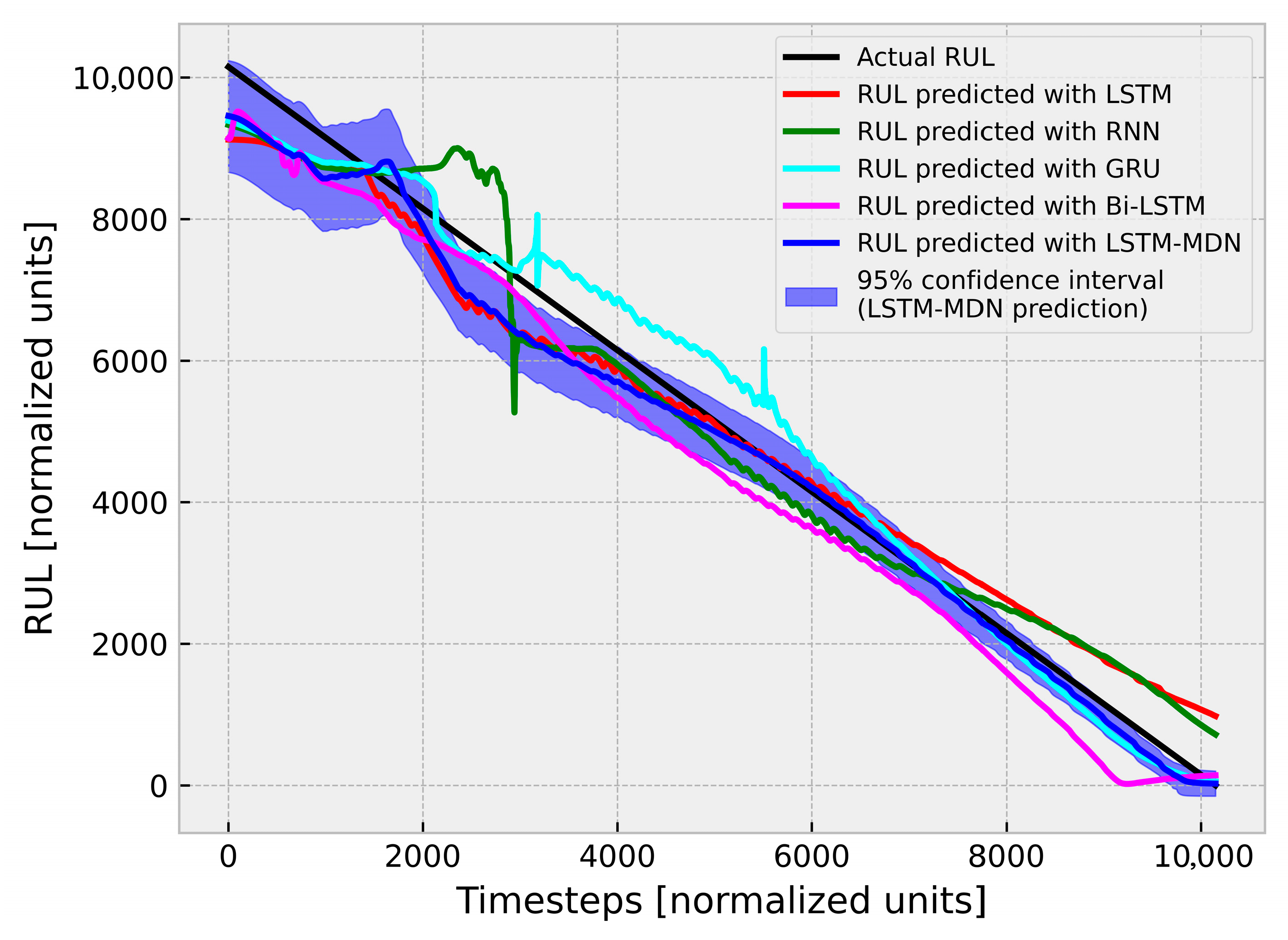
4. Results and Discussion

The predictions of the proposed LSTM-MDN model for the validation IGBT on each iteration during the application of the leave-one-out cross-validation method are depicted in Figure 5, Figure 6, Figure 7 and Figure 8. In addition to the proposed model, the predictions of four different types of recurrent neural networks were also included for comparison purposes: a simple RNN model, a gated recurrent unit (GRU) model, an LSTM model, and a Bi-LSTM model. Only recurrent neural networks have been considered in this comparison because they have already demonstrated better performance and robustness than other models for this type of dataset [26]. The models included in the comparison were created with a similar architecture composed of four layers: a recurrent layer, two fully connected hidden layers, and an output layer. The type of recurrent layer varies between models, but it contains 128 units in all cases. The fully connected hidden layers are equal to those of the LSTM-MDN model, while the output layer of the four models included in the comparison is also fully connected, but with only one unit. For training these four networks, the same hyperparameters were used as for the training of the proposed model.
In general terms, the LSTM-MDN model is capable of predicting, with low error values, the RULs of the devices, exhibiting a similar trend to the ground truth values. This performance is remarkable, especially if it is noticed that, although in each iteration of the leave-one-out cross-validation method there are multiple samples for training, these only belong to three different devices, which could be considered as a few-shot learning setup. Based on the results obtained, the proposed model could be used in a decision-making system to prevent failures, recommending the replacement or maintenance of the device when the lower boundary of the 95% confidence interval of the predicted RUL is less than 1500 cycles. Additionally, it is noticeable that, in general, the 95% confidence interval has a wider range at the beginning of the tests for all the devices, while, towards the end of life, this interval is narrower. This suggests that the proposed model considers its predictions to be more certain as the end of life of the devices is nearer. This phenomenon occurs because, as wear accumulates, degradation patterns become more predictable and the model can better recognize them, reducing uncertainty. Practically, this implies the need for a cautious interpretation of early predictions while enabling more reliable maintenance decisions as the end of life approaches. Another interesting observation is that the RUL profile predicted by the proposed LSMT-MDN model is less prone to sudden changes when compared to the other models. This is especially noticeable, for example, in Figure 5 and Figure 6, where it is possible to observe sharp fluctuations in the prediction curves of the RNN and GRU models, respectively.
A comparison of the R M S E and R 2 metrics for the analyzed models is presented in Table 1. The proposed LSTM-MDN model outperformed the other four networks in both performance indices in all iterations of the leave-one-out cross-validation method. The difference between the results is especially noticeable when device number 3 was used for validation. In this case, the value of R M S E for LSTM-MDN was more than 95 cycles (>21%) lower than for GRU, more than 167 cycles (>32%) lower than for LSTM, and even more than 206 cycles (>36%) lower than for the other two models, while also obtaining the highest R 2 value of all of them. In addition, when comparing the averages of both metrics, it is evident that the proposed LSTM-MDN model has a better prediction capability than the other four networks. The average R M S E of the LSTM-MDN model is more than 84 cycles (>18%), 137 cycles (>26%), 146 cycles (>27%), and 166 cycles (>30%) lower than the average R M S E of the GRU, LSTM, Bi-LSTM, and RNN networks, respectively. In the case of the average R 2 , the proposed model also achieved the best results.
The comparison results indicate that, given its performance, the proposed model is more appropriate for decision-making toward maintenance actions. It is important to highlight that the comparison was made considering the expected values derived from the LSTM-MDN predictions. However, one of the advantages of this model is the inherent information related to the confidence intervals of the predictions, which could also be used to initiate the maintenance action (e.g., if the lower boundary of the 95% confidence interval is lower than a predefined number of cycles). This is not possible to achieve directly with the rest of the models.

5. Conclusions

This work proposed a method for modeling and predicting the remaining useful life of insulated gate bipolar transistors by hybridizing long short-term memory and mixture density networks. By combining the key features of long short-term memory and mixture density network layers in a single neural network architecture, more reliable and informative remaining useful life predictions can be obtained. Validation studies demonstrated that this type of network can effectively estimate the remaining useful life of the devices, and it can even generate convenient confidence intervals for determining the end-of-life of the device in few-shot learning setups, which is very convenient for its assimilation by Industry 4.0 actors. After comparing the proposed model with other well-established methods used for remaining useful life prediction, it was determined that the long short-term memory mixture density network model outperforms them in terms of R M S E and R 2 . The average reduction of the R M S E using the proposed approach was over 84 cycles, which represents an 18% improvement when compared to the second-best performing model. This is a significant result with a potential benefit for critical applications where the remaining useful life of insulated gate bipolar transistors needs to be reliably estimated.
Despite the good results obtained, it must be noticed that they were achieved without using any hyperparameter optimization technique for improving the network performance. Furthermore, the input sequence length used in this study was also preestablished without assessing its impact on the network predictions. Future works will explore the influence of hyperparameters and sequence length on the network performance. Another interesting direction for future work will be the estimation of a health indicator as an intermediate step for RUL prediction, which could improve the interpretability of the results. Additionally, this study opens the path for further research related to the remaining useful life forecast in other fields, where not only do temporal aspects need to be considered, but also the uncertainty of the prediction.

Author Contributions

Conceptualization, Y.J.C. and R.E.H.; methodology, Y.J.C. and R.E.H.; software, Y.J.C. and F.C.; validation, Y.J.C. and F.C.; formal analysis, Y.J.C., F.C. and R.E.H.; investigation, Y.J.C.; resources, R.E.H.; data curation, F.C.; writing—original draft preparation, Y.J.C.; writing—review and editing, F.C. and R.E.H.; visualization, F.C.; supervision, R.E.H.; project administration, R.E.H.; funding acquisition, R.E.H. All authors have read and agreed to the published version of the manuscript.

Funding

This research was funded by the European Union HORIZON Framework Programme and Chips JU, grant number 101096387 for the project “Digitalization of Power Electronic Applications within Key Technology Value Chains (PowerizeD)”, and by MICIU and NextGenerationEU/PRTR, grant number PID2021-127763OB-I00 for the project “Self-reconfiguration for Industrial Cyber-Physical Systems based on digital twins and Artificial Intelligence. Methods and application in Industry 4.0 pilot line”.

Institutional Review Board Statement

Not applicable.

Informed Consent Statement

Not applicable.

Data Availability Statement

The data presented in the study are openly available in the NASA Open Data Portal at https://data.nasa.gov/dataset/insulated-gate-bipolar-transistor-igbt-accelerated-aging (accessed on 13 November 2024).

Conflicts of Interest

The authors declare no conflicts of interest. The funders had no role in the design of the study; in the collection, analyses, or interpretation of data; in the writing of the manuscript; or in the decision to publish the results.

Abbreviations

The following abbreviations are used in this manuscript:
IGBTInsulated Gate Bipolar Transistor
RULRemaining Useful Life
LSTMLong Short-Term Memory
MDNMixture Density Network
CNNConvolutional Neural Network
SVRSupport Vector Regression
GPRGaussian Process Regression
NASANational Aeronautics and Space Administration
Bi-LSTMBi-directional LSTM
RNNRecurrent Neural Network
ARIMAAutoregressive Integrated Moving Average
RMSERoot Mean Squared Error
R2Coefficient of Determination
GRUGated Recurrent Unit

References

  1. Dai, J.; Kim, C.; Mukundhan, P. Applications of Picosecond Laser Acoustics to Power Semiconductor Device: IGBT and MOSFET. In Proceedings of the 2023 China Semiconductor Technology International Conference (CSTIC), Shanghai, China, 17–26 June 2023; pp. 1–3. [Google Scholar]
  2. Zhuang, L.; Xu, A.; Wang, X.-L. A Prognostic Driven Predictive Maintenance Framework Based on Bayesian Deep Learning. Reliab. Eng. Syst. Saf. 2023, 234, 109181. [Google Scholar] [CrossRef]
  3. Wang, K.; Sun, P.; Zhu, B.; Luo, Q.; Du, X. Monitoring Chip Branch Failure in Multichip IGBT Modules Based on Gate Charge. IEEE Trans. Ind. Electron. 2023, 70, 5214–5223. [Google Scholar] [CrossRef]
  4. Wang, Y.; Xie, F.; Zhao, T.; Li, Z.; Li, M.; Liu, D. IGBT Status Prediction Based on PSO-RF with Time-Frequency Domain Features. In Proceedings of the 2022 IEEE 11th Data Driven Control and Learning Systems Conference (DDCLS), Chengdu, China, 3–5 August 2022; pp. 337–341. [Google Scholar]
  5. Cruz, Y.J.; Rivas, M.; Quiza, R.; Beruvides, G.; Haber, R.E. Computer Vision System for Welding Inspection of Liquefied Petroleum Gas Pressure Vessels Based on Combined Digital Image Processing and Deep Learning Techniques. Sensors 2020, 20, 4505. [Google Scholar] [CrossRef] [PubMed]
  6. Cruz, Y.J.; Rivas, M.; Quiza, R.; Villalonga, A.; Haber, R.E.; Beruvides, G. Ensemble of Convolutional Neural Networks Based on an Evolutionary Algorithm Applied to an Industrial Welding Process. Comput. Ind. 2021, 133, 103530. [Google Scholar] [CrossRef]
  7. Sommeregger, L.; Pilz, J. Regularizing Lifetime Drift Prediction in Semiconductor Electrical Parameters with Quantile Random Forest Regression. Technologies 2024, 12, 165. [Google Scholar] [CrossRef]
  8. Perçuku, A.; Minkovska, D.; Hinov, N. Enhancing Electricity Load Forecasting with Machine Learning and Deep Learning. Technologies 2025, 13, 59. [Google Scholar] [CrossRef]
  9. Ali, A.R.; Kamal, H. Time-to-Fault Prediction Framework for Automated Manufacturing in Humanoid Robotics Using Deep Learning. Technologies 2025, 13, 42. [Google Scholar] [CrossRef]
  10. El Bazi, N.; Guennouni, N.; Mekhfioui, M.; Goudzi, A.; Chebak, A.; Mabrouki, M. Predicting the Temperature of a Permanent Magnet Synchronous Motor: A Comparative Study of Artificial Neural Network Algorithms. Technologies 2025, 13, 120. [Google Scholar] [CrossRef]
  11. Alomari, Y.; Andó, M.; Baptista, M.L. Advancing Aircraft Engine RUL Predictions: An Interpretable Integrated Approach of Feature Engineering and Aggregated Feature Importance. Sci. Rep. 2023, 13, 13466. [Google Scholar] [CrossRef] [PubMed]
  12. Zhang, H.; Zhang, S.; Qiu, L.; Zhang, Y.; Wang, Y.; Wang, Z.; Yang, G. A Remaining Useful Life Prediction Method Based on PSR-Former. Sci. Rep. 2022, 12, 17887. [Google Scholar] [CrossRef]
  13. Liu, K.; Shang, Y.; Ouyang, Q.; Widanage, W.D. A Data-Driven Approach With Uncertainty Quantification for Predicting Future Capacities and Remaining Useful Life of Lithium-Ion Battery. IEEE Trans. Ind. Electron. 2021, 68, 3170–3180. [Google Scholar] [CrossRef]
  14. Chechkin, A.; Pleshakova, E.; Gataullin, S. A Hybrid KAN-BiLSTM Transformer with Multi-Domain Dynamic Attention Model for Cybersecurity. Technologies 2025, 13, 223. [Google Scholar] [CrossRef]
  15. Zhao, Z.; Wu, J.; Wong, D.; Sun, C.; Yan, R. Probabilistic Remaining Useful Life Prediction Based on Deep Convolutional Neural Network. In Proceedings of the 9th International Conference on Through-life Engineering Services (TESConf 2020), Cranfield, UK, 3-4 November 2020. [Google Scholar]
  16. Zhao, D.; Liu, F. Cross-Condition and Cross-Platform Remaining Useful Life Estimation via Adversarial-Based Domain Adaptation. Sci. Rep. 2022, 12, 878. [Google Scholar] [CrossRef] [PubMed]
  17. Kerin, M.; Hartono, N.; Pham, D.T. Optimising Remanufacturing Decision-Making Using the Bees Algorithm in Product Digital Twins. Sci. Rep. 2023, 13, 701. [Google Scholar] [CrossRef]
  18. Unni, R.; Yao, K.; Zheng, Y. Deep Convolutional Mixture Density Network for Inverse Design of Layered Photonic Structures. ACS Photonics 2020, 7, 2703–2712. [Google Scholar] [CrossRef] [PubMed]
  19. Li, W.; Wang, B.; Liu, J.; Zhang, G.; Wang, J. IGBT Aging Monitoring and Remaining Lifetime Prediction Based on Long Short-Term Memory (LSTM) Networks. Microelectron. Reliab. 2020, 114, 113902. [Google Scholar] [CrossRef]
  20. Ma, L.; Huang, J.; Chai, X.; He, S. Life Prediction for IGBT Based on Improved Long Short-Term Memory Network. In Proceedings of the 2023 IEEE 18th Conference on Industrial Electronics and Applications (ICIEA), Ningbo, China, 18–22 August 2023; pp. 868–873. [Google Scholar]
  21. Wang, X.; Zhou, Z.; He, S.; Liu, J.; Cui, W. Performance Degradation Modeling and Its Prediction Algorithm of an IGBT Gate Oxide Layer Based on a CNN-LSTM Network. Micromachines 2023, 14, 959. [Google Scholar] [CrossRef] [PubMed]
  22. Du, X.; Li, Y. Remaining Useful Life Prediction for IGBT Based on SO-Bi- ALSTM. In Proceedings of the 2023 IEEE 9th International Conference on Cloud Computing and Intelligent Systems (CCIS), Dali, China, 12–13 August 2023; pp. 193–198. [Google Scholar]
  23. Lu, Z.; Guo, C.; Liu, M.; Shi, R. Remaining Useful Lifetime Estimation for Discrete Power Electronic Devices Using Physics-Informed Neural Network. Sci. Rep. 2023, 13, 10167. [Google Scholar] [CrossRef] [PubMed]
  24. Yousuf, S.; Khan, S.A.; Khursheed, S. Remaining Useful Life (RUL) Regression Using Long–Short Term Memory (LSTM) Networks. Microelectron. Reliab. 2022, 139, 114772. [Google Scholar] [CrossRef]
  25. Castano, F.; Cruz, Y.J.; Villalonga, A.; Haber, R.E. Data-Driven Insights on Time-to-Failure of Electromechanical Manufacturing Devices: A Procedure and Case Study. IEEE Trans. Industr. Inform. 2023, 19, 7190–7200. [Google Scholar] [CrossRef]
  26. Chen, Z.; Wu, M.; Zhao, R.; Guretno, F.; Yan, R.; Li, X. Machine Remaining Useful Life Prediction via an Attention-Based Deep Learning Approach. IEEE Trans. Ind. Electron. 2021, 68, 2521–2531. [Google Scholar] [CrossRef]
  27. Fei, Z.; Huang, Z.; Zhang, X. Voltage and Temperature Information Ensembled Probabilistic Battery Health Evaluation via Deep Gaussian Mixture Density Network. J. Energy Storage 2023, 73, 108587. [Google Scholar] [CrossRef]
  28. Kim, G.; Yang, S.M.; Kim, S.; Kim, D.Y.; Choi, J.G.; Park, H.W.; Lim, S. A Multi-Domain Mixture Density Network for Tool Wear Prediction under Multiple Machining Conditions. Int. J. Prod. Res. 2023, 1–20, 2289076. [Google Scholar] [CrossRef]
  29. Bazzani, L.; Larochelle, H.; Torresani, L. Recurrent Mixture Density Network for Spatiotemporal Visual Attention. arXiv 2017, arXiv:1603.08199. [Google Scholar] [CrossRef]
  30. Zhao, Y.; Yang, R.; Chevalier, G.; Shah, R.C.; Romijnders, R. Applying Deep Bidirectional LSTM and Mixture Density Network for Basketball Trajectory Prediction. Optik 2018, 158, 266–272. [Google Scholar] [CrossRef]
  31. Felder, M.; Kaifel, A.; Graves, A. Wind Power Prediction Using Mixture Density Recurrent Neural Networks. In Proceedings of the European Wind Energy Conference & Exhibition 2010 (EWEC 2010), Warsaw, Poland, 20-23 April 2010; pp. 3417–3424. [Google Scholar]
  32. Mukherjee, S.; Shankar, D.; Ghosh, A.; Tathawadekar, N.; Kompalli, P.; Sarawagi, S.; Chaudhury, K. ARMDN: Associative and Recurrent Mixture Density Networks for ERetail Demand Forecasting. arXiv 2018, arXiv:1803.03800. [Google Scholar] [CrossRef]
  33. Schwab, D.; O’Rourke, S.M.; Minnehan, B.L. Combining LSTM and MDN Networks for Traffic Forecasting Using the Argoverse Dataset. In Proceedings of the 2021 IEEE 24th International Conference on Information Fusion (FUSION), Sun City, South Africa, 1–4 November 2021; pp. 1–6. [Google Scholar]
  34. Chen, M.; Chen, R.; Cai, F.; Li, W.; Guo, N.; Li, G. Short-Term Traffic Flow Prediction with Recurrent Mixture Density Network. Math. Probl. Eng. 2021, 2021, 6393951. [Google Scholar] [CrossRef]
  35. Gugulothu, N.; Subramanian, E.; Bhat, S.P. Sparse Recurrent Mixture Density Networks for Forecasting High Variability Time Series with Confidence Estimates. In Artificial Neural Networks and Machine Learning—ICANN 2019: Deep Learning: 28th International Conference on Artificial Neural Networks, Munich, Germany, September 17–19, 2019, Proceedings, Part II; Springer: Berlin/Heidelberg, Germany, 2019; pp. 422–433. ISBN 978-3-030-30483-6. [Google Scholar]
  36. Lei, Y.; Karimi, H.R.; Chen, X. A Novel Self-Supervised Deep LSTM Network for Industrial Temperature Prediction in Aluminum Processes Application. Neurocomputing 2022, 502, 177–185. [Google Scholar] [CrossRef]
  37. Hochreiter, S.; Schmidhuber, J. Long Short-Term Memory. Neural Comput. 1997, 9, 1735–1780. [Google Scholar] [CrossRef] [PubMed]
  38. Zhang, H.; Liu, Y.; Yan, J.; Han, S.; Li, L.; Long, Q. Improved Deep Mixture Density Network for Regional Wind Power Probabilistic Forecasting. IEEE Trans. Power Syst. 2020, 35, 2549–2560. [Google Scholar] [CrossRef]
  39. Bishop, C.M. Mixture Density Networks; Aston University: Birmingham, UK, 1994. [Google Scholar]
  40. Celaya, J.; Wysocki, P.; Goebel, K. IGBT Accelerated Aging Data Set; NASA Prognostics Data Repository; NASA Ames Research Center: Moffett Field, CA, USA, 2009. [Google Scholar]
  41. Xiao, D.; Qin, C.; Ge, J.; Xia, P.; Huang, Y.; Liu, C. Self-Attention-Based Adaptive Remaining Useful Life Prediction for IGBT with Monte Carlo Dropout. Knowl. Based Syst. 2022, 239, 107902. [Google Scholar] [CrossRef]
  42. Boutrous, K.; Bessa, I.; Puig, V.; Nejjari, F.; Palhares, R.M. Data-Driven Prognostics Based on Evolving Fuzzy Degradation Models for Power Semiconductor Devices. PHM Soc. Eur. Conf. 2022, 7, 68–77. [Google Scholar] [CrossRef]
  43. Ismail, A.; Saidi, L.; Sayadi, M.; Benbouzid, M. A New Data-Driven Approach for Power IGBT Remaining Useful Life Estimation Based On Feature Reduction Technique and Neural Network. Electronics 2020, 9, 1571. [Google Scholar] [CrossRef]
  44. Ge, J.; Huang, Y.; Tao, Z.; Li, B.; Xiao, D.; Li, Y.; Liu, C. RUL Predict of IGBT Based on DeepAR Using Transient Switch Features. PHM Soc. Eur. Conf. 2020, 5, 11. [Google Scholar] [CrossRef]
  45. Cruz, Y.J.; Castaño, F.; Haber, R.E.; Villalonga, A.; Ejsmont, K.; Gladysz, B.; Flores, Á.; Alemany, P. Self-Reconfiguration for Smart Manufacturing Based on Artificial Intelligence: A Review and Case Study BT—Artificial Intelligence in Manufacturing: Enabling Intelligent, Flexible and Cost-Effective Production Through AI; Soldatos, J., Ed.; Springer Nature: Cham, Switzerland, 2024; pp. 121–144. ISBN 978-3-031-46452-2. [Google Scholar]
  46. Cruz, Y.J.; Villalonga, A.; Castaño, F.; Rivas, M.; Haber, R.E. Automated Machine Learning Methodology for Optimizing Production Processes in Small and Medium-Sized Enterprises. Oper. Res. Perspect. 2024, 12, 100308. [Google Scholar] [CrossRef]
Figure 1. Unrolled representation of an LSTM cell.
Technologies 13 00321 g001
Figure 2. Gaussian mixture.
Technologies 13 00321 g002
Figure 3. LSTM-MDN architecture.
Technologies 13 00321 g003
Figure 4. Failure point of device 3.
Technologies 13 00321 g004
Figure 5. Predicted RUL when device 2 was used for validation in the leave-one-out cross-validation method.
Technologies 13 00321 g005
Figure 6. Predicted RUL when device 3 was used for validation in the leave-one-out cross-validation method.
Technologies 13 00321 g006
Figure 7. Predicted RUL when device 4 was used for validation in the leave-one-out cross-validation method.
Technologies 13 00321 g007
Figure 8. Predicted RUL when device 5 was used for validation in the leave-one-out cross-validation method.
Technologies 13 00321 g008
Table 1. Comparison of the proposed model versus other techniques.
ModelRNNGRULSTMBi-LSTMLSTM-MDN
(Our Approach)
Validation device2 R M S E (cycles)543.72453.83514.53561.26384.33
R 2 0.960.980.960.960.98
3 R M S E (cycles)558.99447.81520.16593.89352.27
R 2 0.960.980.970.950.98
4 R M S E (cycles)534.18416.52544.11460.60381.50
R 2 0.960.980.960.970.98
5 R M S E (cycles)542.85534.68522.75450.06396.89
R 2 0.960.960.960.970.98
Average R M S E (cycles)544.94463.21525.39516.45378.75
R 2 0.960.980.960.960.98
Disclaimer/Publisher’s Note: The statements, opinions and data contained in all publications are solely those of the individual author(s) and contributor(s) and not of MDPI and/or the editor(s). MDPI and/or the editor(s) disclaim responsibility for any injury to people or property resulting from any ideas, methods, instructions or products referred to in the content.

