
Non-Contact Oxygen Saturation Estimation Using Deep Learning Ensemble Models and Bayesian Optimization


Abstract
1. Introduction
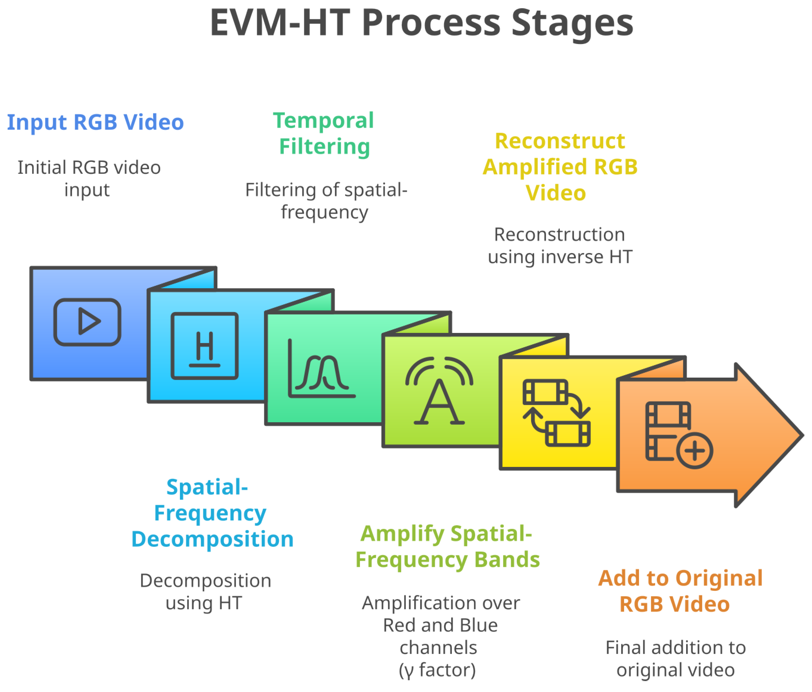
- EVM-HT approach:
- -
- We used the EVM-HT method as a feature detector, which is used as input by the 3D-CNN to estimate the SpO2.
- -
- This makes it easier for the 3D-CNN to focus on those regions where there are chrominance changes.
- New DL combined strategy to estimate SpO2:
- -
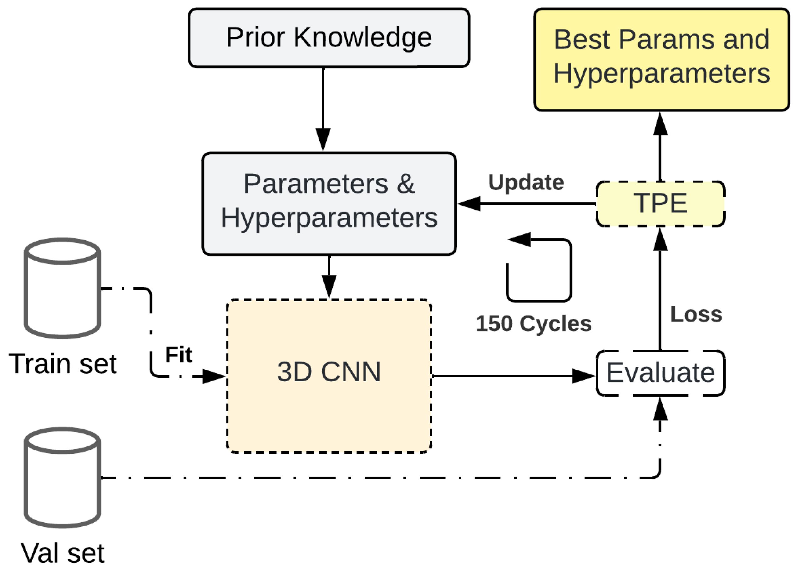
- We applied a Bayesian optimization approach to reduce the training error or bias compared to our previous baseline CNN model [29].
- -
- We used the Bagging technique to achieve a better generalization over the test set with respect to the optimized model, which reduces the variance.
- No calibration required per subject:
- -
- In the proposed DL SpO2-estimation approach, a calibration process per subject is not necessary, allowing its implementation in real conditions.
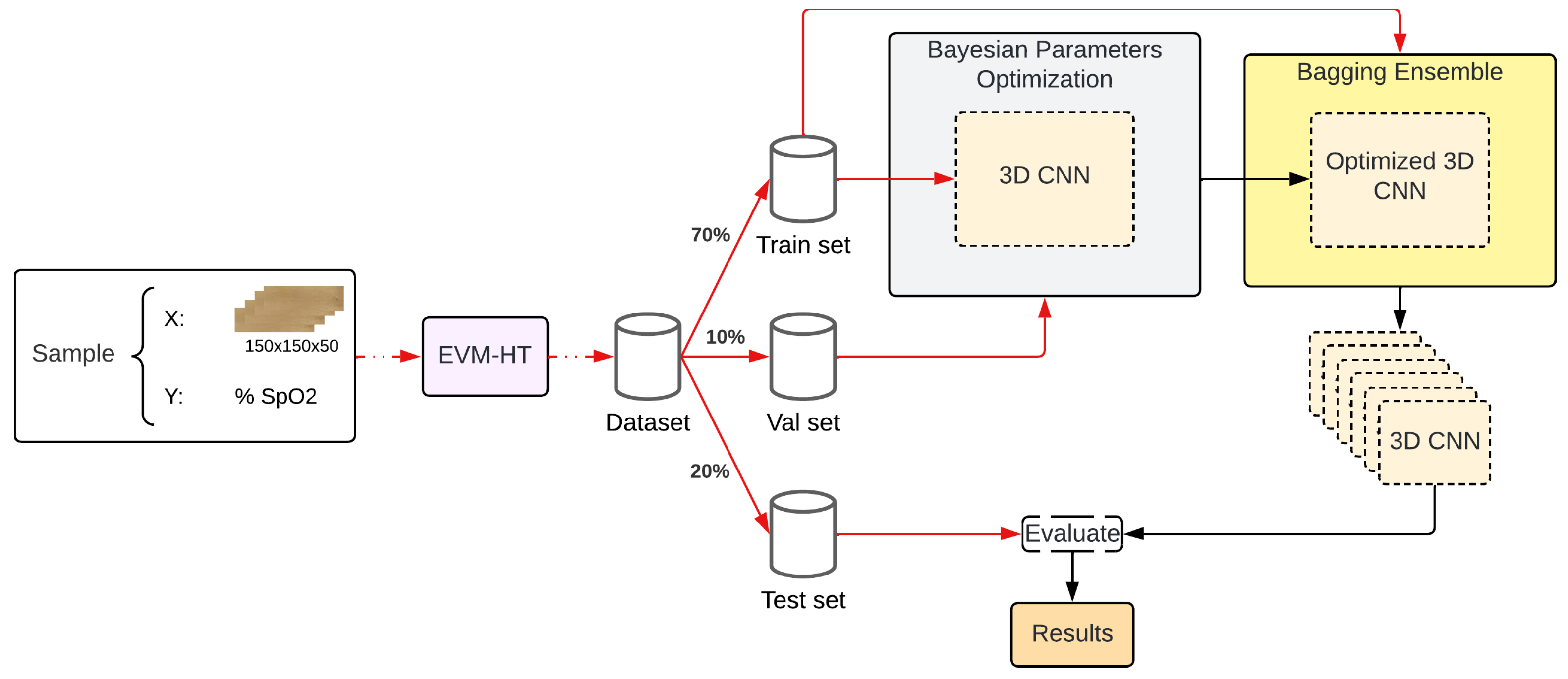
2. Materials and Methods
2.1. Experimental Setup
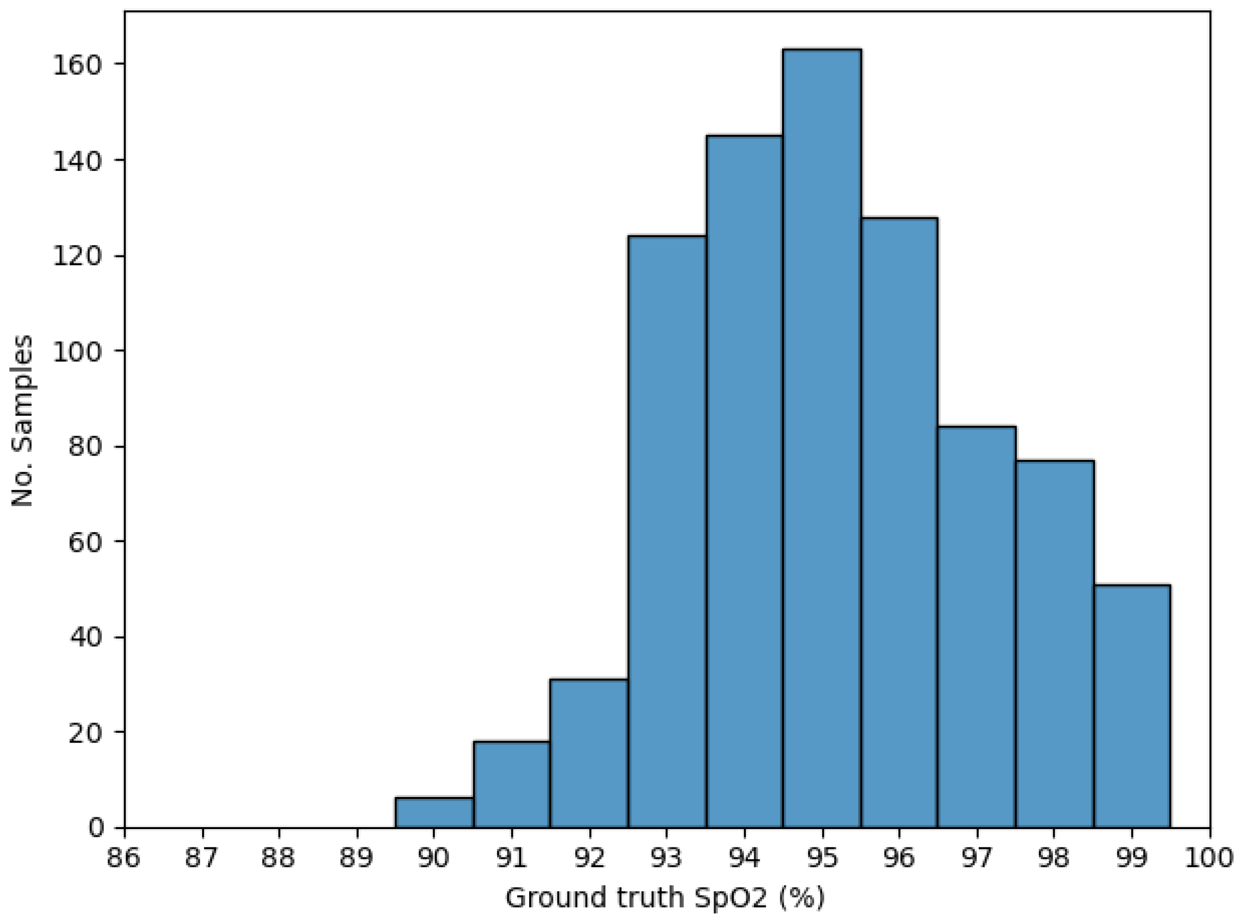
2.2. Dataset
2.3. Eulerian Video Magnification Technique Using Hermite Transform
2.4. Data Processing
- 150 ROI batches were generated by stacking ROIs from the dataset. The target for each batch was derived from the oximeter value in the final frame.
- A 125-ROI sliding window technique was used as a data-augmentation strategy.
- To ensure a consistent input size, each ROI was resized to .
- A split ratio of 70-10-20 was applied to divide the dataset into training, validation, and testing sets.
- The target was normalized with mean and standard deviation.
2.5. Model Architecture
2.6. Parameter Optimization
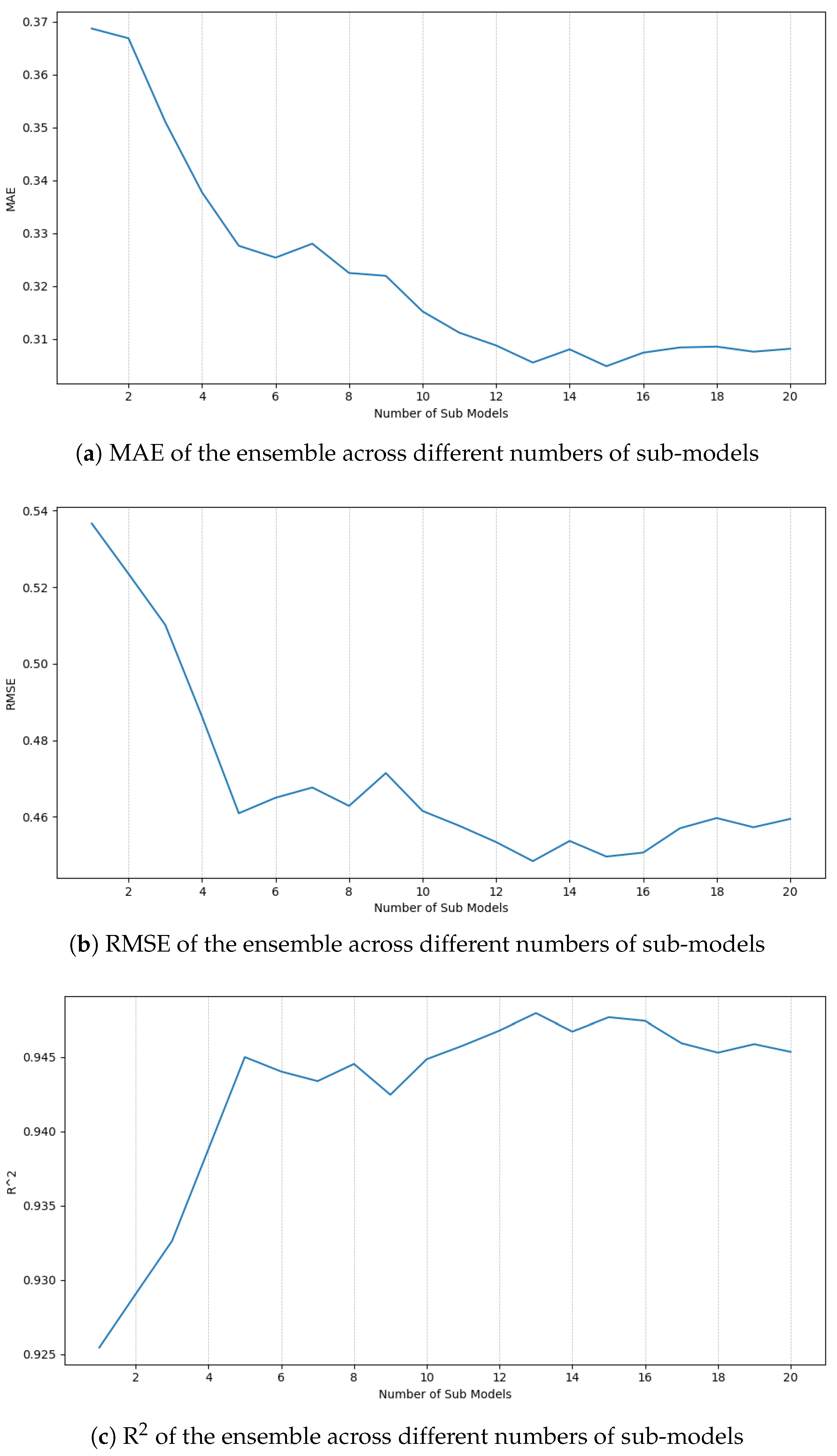
2.7. Bagging Ensemble
3. Results
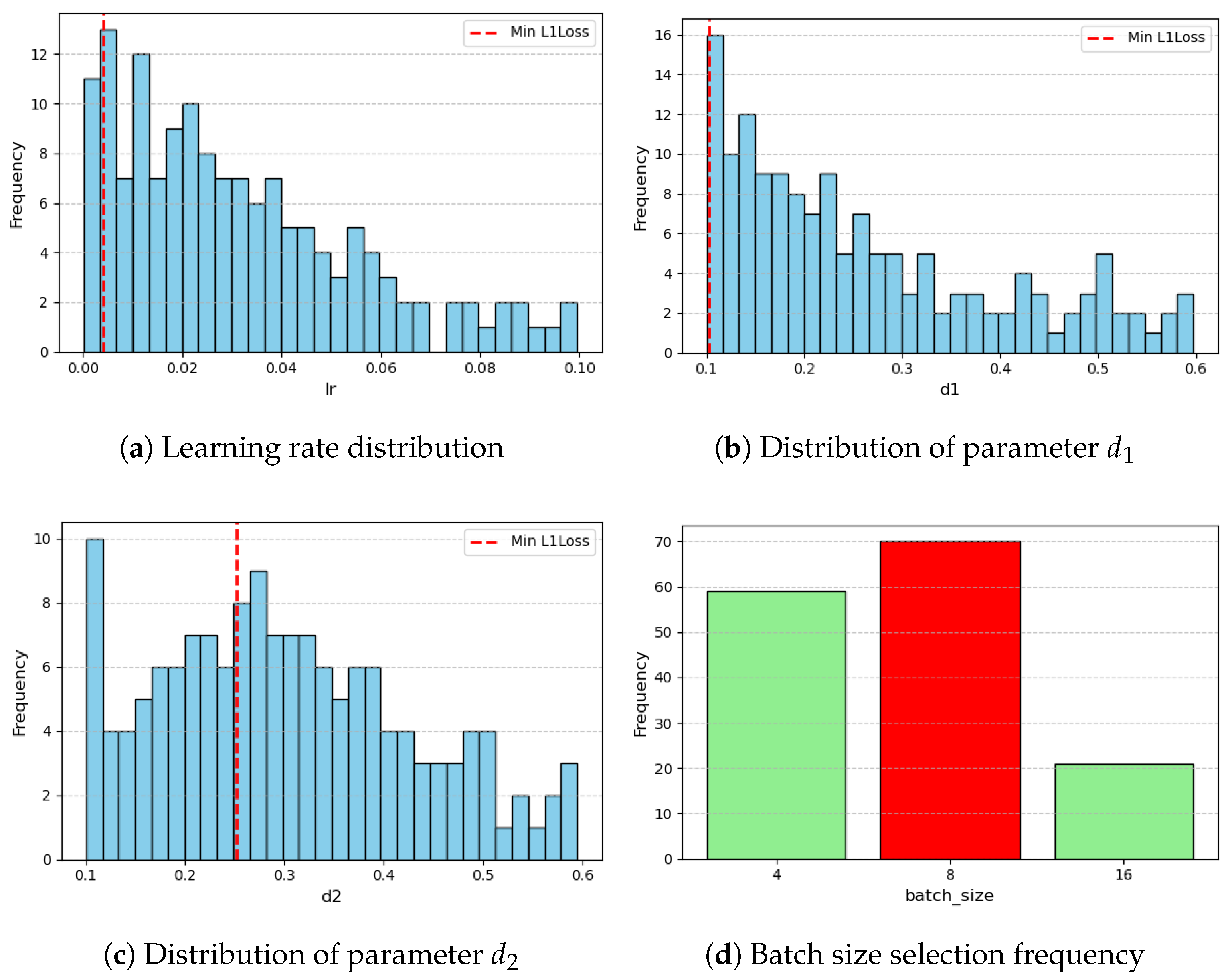
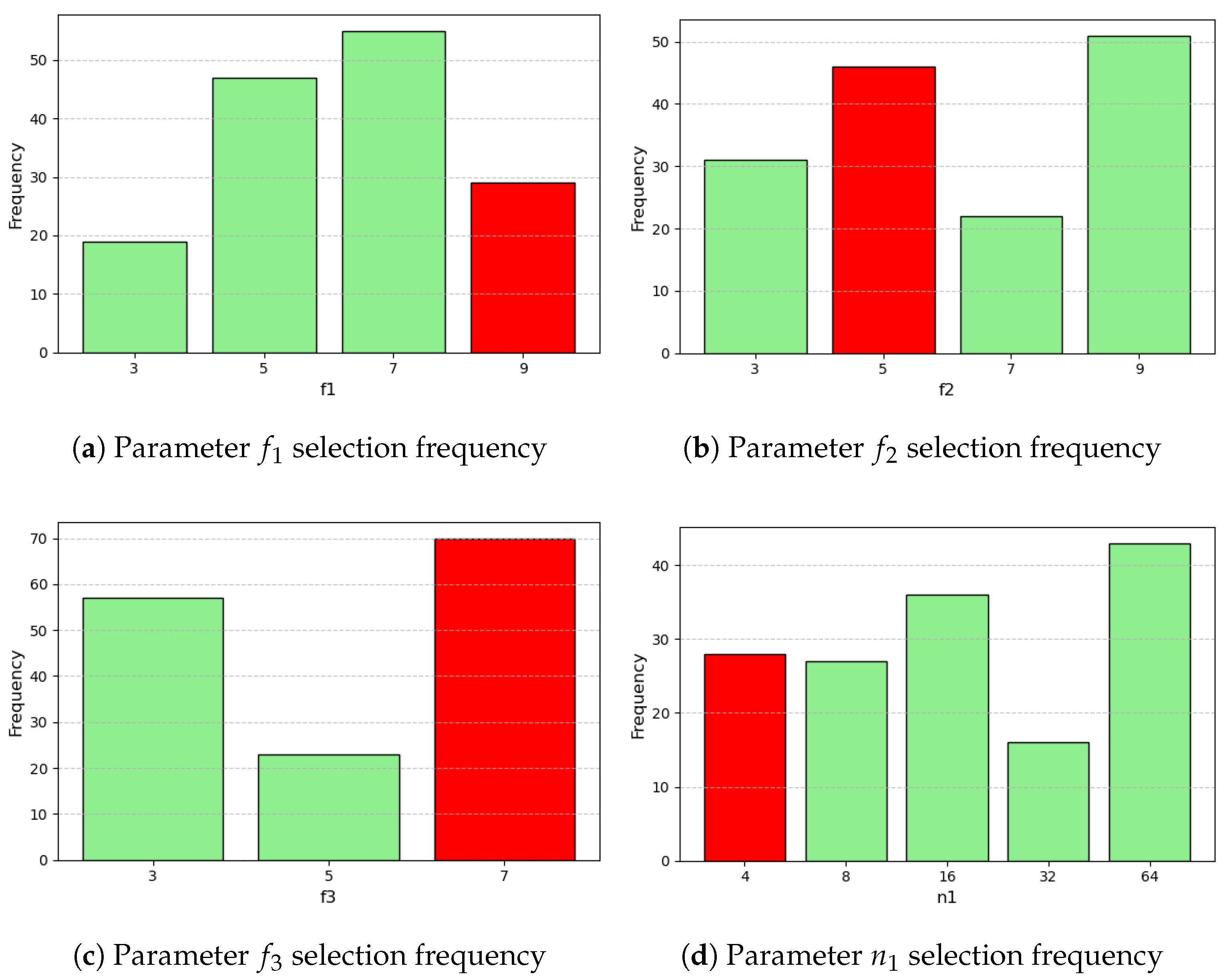
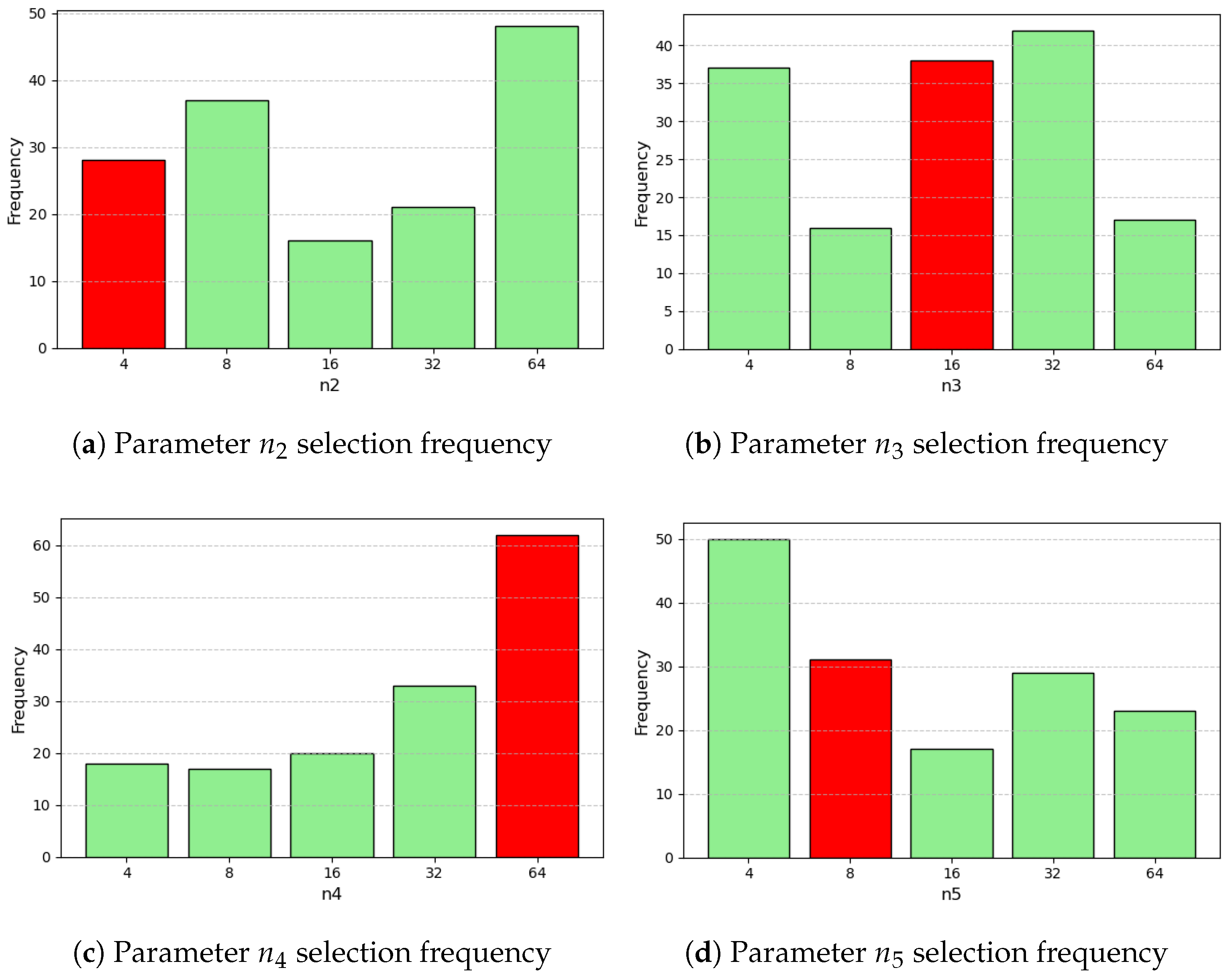
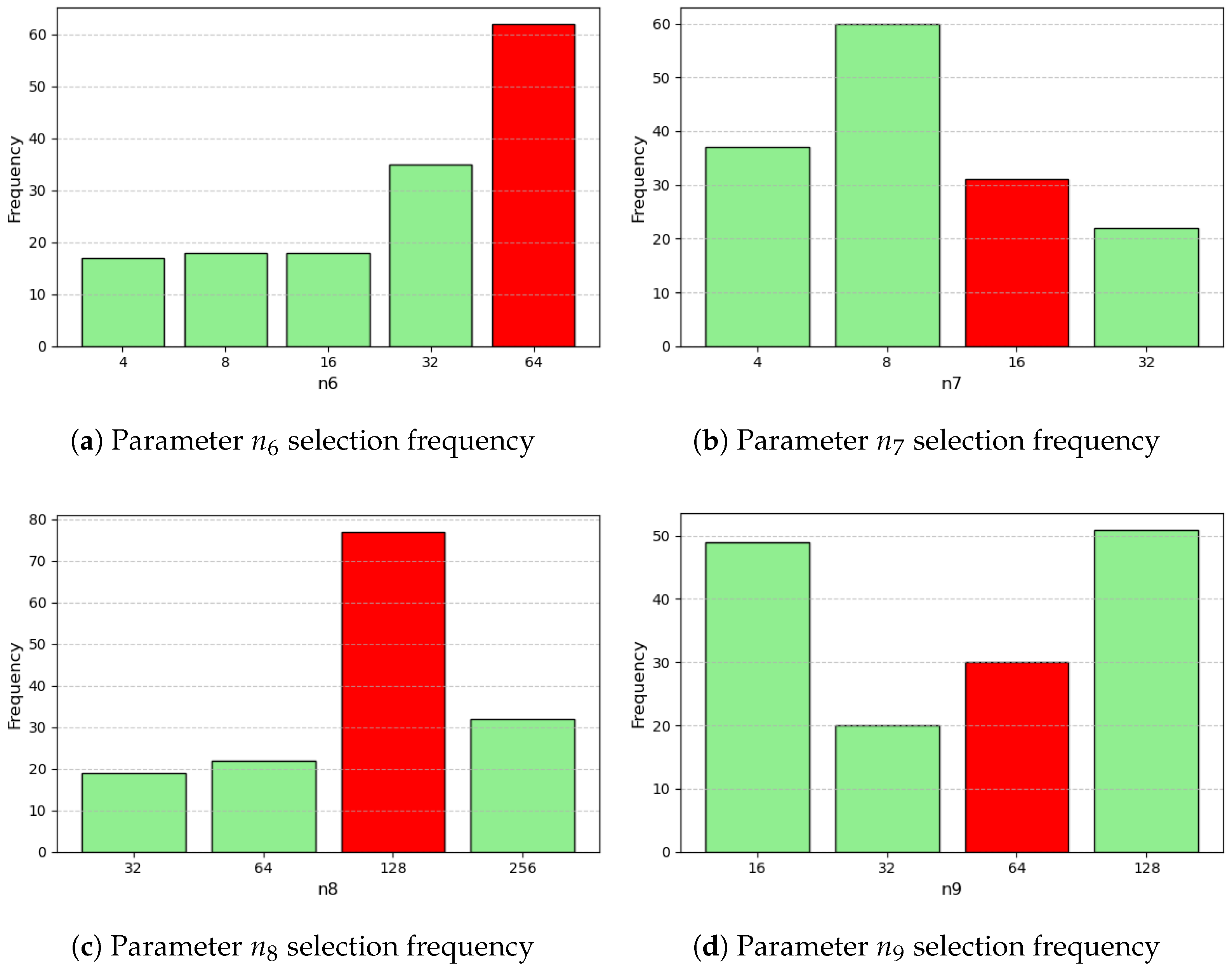
3.1. Parameter Optimization
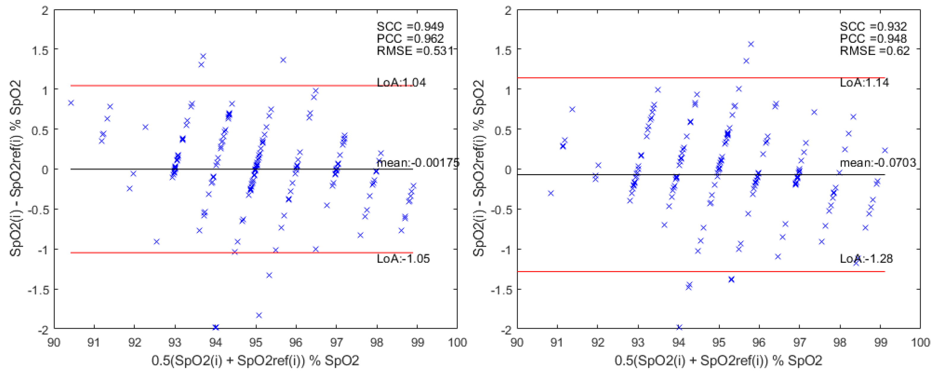
3.2. Bagging Ensemble
4. Discussion
5. Conclusions
Author Contributions
Funding
Institutional Review Board Statement
Informed Consent Statement
Data Availability Statement
Acknowledgments
Conflicts of Interest
Abbreviations
| BA | Bland–Altman |
| bmp | beats per minute |
| CNN | Convolutional Neural Networks |
| 3D-CNN | Three-Dimensional Convolutional Neural Network |
| CCM | Color Channel Model |
| COVID-19 | Coronavirus Disease 2019 |
| DL | Deep Learning |
| DS | Dynamic Spectrum |
| EEMD | Ensemble Empirical Mode Decomposition |
| EVM | Eulerian Video Magnification |
| EVM-HT | Eulerian Video Magnification - Hermite Transform |
| FCL | Fully Connected Layer |
| ICA | Independent Component Analysis |
| ICU | Intensive Care Unit |
| LoA | Limits of Agreement |
| LSTM | Long Short- Term Memory |
| ML | Machine Learning |
| MCML | Monte Carlo Modeling |
| MAE | Mean Absolute Error |
| MOD | Mean of Differences |
| MS | Monte Carlo Simulation |
| NL | Normalization Layer |
| PCC | Pearson’s Correlation Coefficient |
| PLS | Partial Least Squares |
| PPG | Photoplethysmography |
| RCA | Residual and Coordinate Attention |
| RMSE | Root Mean Square Error |
| rPPG | remote Photoplethysmography |
| R2 | Coefficient of Determination |
| RL | Residual Layer |
| ROI | Region Of Interest |
| SARS-CoV-2 | Severe Acute Respiratory Syndrome Coronavirus 2 |
| SBMO | Sequential Model-Based Optimization |
| SCC | Spearman Correlation Coefficient |
| SGD | Stochastic gradient descent |
| SpO2 | Peripheral Oxygen Saturation |
| SVR | Support Vector Regression |
| TPE | Tree-structured Parzen Estimator |
| ViT | Video Vision Transformer |
| VIS-NIR | Visible–near infrared |
Appendix A
References
- Hackett, K. Guidance on oxygen use in adults. Emerg. Nurse J. RCN Accid. Emerg. Nurs. Assoc. 2017, 25, 11. [Google Scholar] [CrossRef] [PubMed]
- Paules, C.I.; Marston, H.D.; Fauci, A.S. Coronavirus Infections—More Than Just the Common Cold. JAMA 2020, 323, 707–708. [Google Scholar] [CrossRef] [PubMed]
- Struyf, T.; Deeks, J.J.; Dinnes, J.; Takwoingi, Y.; Davenport, C.; Leeflang, M.M.; Spijker, R.; Hooft, L.; Emperador, D.; Dittrich, S.; et al. Signs and symptoms to determine if a patient presenting in primary care or hospital outpatient settings has COVID-19 disease. Cochrane Database Syst. Rev. 2020, 7, CD013665. [Google Scholar] [CrossRef] [PubMed]
- Moro, E.; Priori, A.; Beghi, E.; Helbok, R.; Campiglio, L.; Bassetti, C.L.; Bianchi, E.; Maia, L.F.; Ozturk, S.; Cavallieri, F.; et al. The international European Academy of Neurology survey on neurological symptoms in patients with COVID-19 infection. Eur. J. Neurol. 2020, 27, 1727–1737. [Google Scholar] [CrossRef] [PubMed]
- Hajr, A.; Tarvirdizadeh, B.; Alipour, K.; Ghamari, M. Contactless Health Monitoring: An Overview of Video-Based Techniques Utilising Machine/Deep Learning. IET Wirel. Sens. Syst. 2025, 15, e70009. [Google Scholar] [CrossRef]
- Poh, M.Z.; McDuff, D.; Picard, R. Non-contact, automated cardiac pulse measurements using video imaging and blind source separation. Opt. Express 2010, 18, 10762–10774. [Google Scholar] [CrossRef] [PubMed]
- Moya-Albor, E.; Brieva, J.; Ponce, H.; Martínez-Villaseñor, L. A non-contact heart rate estimation method using video magnification and neural networks. IEEE Instrum. Meas. Mag. 2020, 23, 56–62. [Google Scholar] [CrossRef]
- Liu, X.; Zhang, Y.; Yu, Z.; Lu, H.; Yue, H.; Yang, J. rppg-mae: Self-supervised pretraining with masked autoencoders for remote physiological measurements. IEEE Trans. Multimed. 2024, 26, 7278–7293. [Google Scholar] [CrossRef]
- Othman, W.; Kashevnik, A.; Ali, A.; Shilov, N.; Ryumin, D. Remote heart rate estimation based on transformer with multi-skip connection decoder: Method and evaluation in the wild. Sensors 2024, 24, 775. [Google Scholar] [CrossRef] [PubMed]
- Wang, R.X.; Sun, H.M.; Hao, R.R.; Pan, A.; Jia, R.S. TransPhys: Transformer-based unsupervised contrastive learning for remote heart rate measurement. Biomed. Signal Process. Control 2023, 86, 105058. [Google Scholar] [CrossRef]
- Cheng, C.H.; Wong, K.L.; Chin, J.W.; Chan, T.T.; So, R.H. Deep learning methods for remote heart rate measurement: A review and future research agenda. Sensors 2021, 21, 6296. [Google Scholar] [CrossRef] [PubMed]
- Brieva, J.; Ponce, H.; Moya-Albor, E. A contactless respiratory rate estimation method using a hermite magnification technique and convolutional neural networks. Appl. Sci. 2020, 10, 607. [Google Scholar] [CrossRef]
- Bian, D.; Mehta, P.; Selvaraj, N. Respiratory rate estimation using PPG: A deep learning approach. In Proceedings of the 2020 42nd Annual International Conference of the IEEE Engineering in Medicine & Biology Society (EMBC), Montreal, QC, Canada, 20–24 July 2020; IEEE: Piscataway, NJ, USA, 2020; pp. 5948–5952. [Google Scholar]
- Hashim, H.A. Non-Contact Automatic Respiratory Rate Monitoring for Newborns Using Digital Camera Technology and Deep Learning. J. Biomed. Photonics Eng. 2024, 10, 040317-1–040317-12. [Google Scholar] [CrossRef]
- Lee, H.; Lee, J.; Kwon, Y.; Kwon, J.; Park, S.; Sohn, R.; Park, C. Multitask siamese network for remote photoplethysmography and respiration estimation. Sensors 2022, 22, 5101. [Google Scholar] [CrossRef] [PubMed]
- Wieringa, F.P.; Mastik, F.; van der Steen, A.F.W. Contactless multiple wavelength photoplethysmographic imaging: A first step toward “SpO2 camera” technology. Ann. Biomed. Eng. 2005, 33, 1034–1041. [Google Scholar] [CrossRef] [PubMed]
- Tonmoy, A.S.; Ahmed, M.S.; Chowdhury, A.; Chowdhury, M.H. Estimation of Oxygen Saturation from PPG Signal using Smartphone Recording. In Proceedings of the 2024 International Conference on Advances in Computing, Communication, Electrical, and Smart Systems: Innovation for Sustainability, iCACCESS 2024, Dhaka, Bangladesh, 8–9 March 2024. [Google Scholar] [CrossRef]
- Al-Naji, A.; Khalid, G.; Mahdi, J.; Chahl, J. Non-Contact SpO2 Prediction System Based on a Digital Camera. Appl. Sci. 2021, 11, 4255. [Google Scholar] [CrossRef]
- De Fatima Galvao Rosa, A.; Betini, R. Noncontact SpO2 Measurement Using Eulerian Video Magnification. IEEE Trans. Instrum. Meas. 2020, 69, 2120–2130. [Google Scholar] [CrossRef]
- Wu, B.J.; Wu, B.F.; Dong, Y.C.; Lin, H.C.; Li, P.H. Peripheral Oxygen Saturation Measurement Using an RGB Camera. IEEE Sensors J. 2023, 23, 26551–26563. [Google Scholar] [CrossRef]
- Brieva, J.; Moya-Albor, E.; Ponce, H. A non-contact SpO2 estimation using a video magnification technique. In Proceedings of the 17th International Symposium on Medical Information Processing and Analysis, Campinas, Brazil, 17–19 November 2021; Rittner, L., Romero Castro, E., Lepore, N., Brieva, J., Linguraru, M.G., Eds.; International Society for Optics and Photonics. SPIE: Bellingham, WA, USA, 2021; Volume 12088, pp. 10–18. [Google Scholar] [CrossRef]
- Yaythish Kannaa, G.; Bhattacharya, S.; Aishwarya, N. Remote Photoplethysmography (rPPG) for Contactless Blood Oxygen Saturation Monitoring. In Proceedings of the 2024 IEEE International Conference on Electronics, Computing and Communication Technologies (CONECCT), Bangalore, India, 12–14 July 2024. [Google Scholar] [CrossRef]
- Nakagawa, K.; Kawamoto, H.; Sankai, Y. Noncontact Measurement of Oxygen Saturation with Dual Near Infrared Imaging for Daily Health Monitoring. In Proceedings of the 2022 IEEE/SICE International Symposium on System Integration (SII), Narvik, Norway, 9–12 January 2022; pp. 736–741. [Google Scholar] [CrossRef]
- Lan, T.; Li, G.; Lin, L. A non-contact oxygen saturation detection method based on dynamic spectrum. Infrared Phys. Technol. 2022, 127, 104421. [Google Scholar] [CrossRef] [PubMed]
- Takahashi, R.; Ashida, K.; Kobayashi, Y.; Tokunaga, R.; Kodama, S.; Tsumura, N. Oxygen saturation estimation based on optimal band selection from multi-band video. In Proceedings of the 2021 IEEE/CVF Conference on Computer Vision and Pattern Recognition Workshops (CVPRW), Nashville, TN, USA, 19–25 June 2021; pp. 3845–3851. [Google Scholar] [CrossRef]
- Cheng, C.H.; Yuen, Z.; Chen, S.; Wong, K.L.; Chin, J.W.; Chan, T.T.; So, R.H.Y. Contactless Blood Oxygen Saturation Estimation from Facial Videos Using Deep Learning. Bioengineering 2024, 11, 251. [Google Scholar] [CrossRef] [PubMed]
- Wang, L.; Chen, Z.; Alić, B.; Wildenauer, A.; Dietz-Terjung, S.; Sucre, J.G.O.; Sutharsan, S.; Schöbel, C.; Seidl, K.; Notni, G. Leveraging 3D Convolutional Neural Network and 3D visible-near-infrared multimodal imaging for enhanced contactless oximetry. J. Biomed. Opt. 2024, 29, S33309. [Google Scholar] [CrossRef]
- Stogiannopoulos, T.; Cheimariotis, G.A.; Mitianoudis, N. A non-contact SpO2 estimation using video magnification and infrared data. In Proceedings of the ICASSP 2023–2023 IEEE International Conference on Acoustics, Speech and Signal Processing (ICASSP), Rhodes Island, Greece, 4–10 June 2023. [Google Scholar] [CrossRef]
- Escobedo-Gordillo, A.; Brieva, J.; Moya-Albor, E.; Ponce, H. A non-contact oxygen saturation estimation using Video Magnification and a Deep Learning method. In Proceedings of the 2023 19th International Symposium on Medical Information Processing and Analysis (SIPAIM), Mexico City, Mexico, 15–17 November 2023; pp. 1–6. [Google Scholar] [CrossRef]
- Stogiannopoulos, T.; Cheimariotis, G.A.; Mitianoudis, N. A Study of Machine Learning Regression Techniques for Non-Contact SpO2 Estimation from Infrared Motion-Magnified Facial Video. Information 2023, 14, 301. [Google Scholar] [CrossRef]
- Hu, M.; Wu, X.; Wang, X.; Xing, Y.; An, N.; Shi, P. Contactless blood oxygen estimation from face videos: A multi-model fusion method based on deep learning. Biomed. Signal Process. Control 2023, 81, 104487. [Google Scholar] [CrossRef] [PubMed]
- Akamatsu, Y.; Onishi, Y.; Imaoka, H. Blood oxygen saturation estimation from facial video via dc and ac components of spatio-temporal map. In Proceedings of the ICASSP 2023-2023 IEEE International Conference on Acoustics, Speech and Signal Processing (ICASSP), Rhodes Island, Greece, 4–10 June 2023; IEEE: Piscataway, NJ, USA, 2023; pp. 1–5. [Google Scholar]
- Shao, Q.; Zhu, L.; Ahmed, M.; Vatanparvar, K.; Gwak, M.; Rashid, N.; Bae, J.; Kuang, J.; Gao, A. Normalization is All You Need: Robust Full-Range Contactless SpO2 Estimation Across Users. In Proceedings of the ICASSP 2024–2024 IEEE International Conference on Acoustics, Speech and Signal Processing (ICASSP), Seoul, Republic of Korea, 14–19 April 2024; pp. 1646–1650. [Google Scholar] [CrossRef]
- Cheng, J.C.; Pan, T.S.; Hsiao, W.C.; Lin, W.H.; Liu, Y.L.; Su, T.J.; Wang, S.M. Using Contactless Facial Image Recognition Technology to Detect Blood Oxygen Saturation. Bioengineering 2023, 10, 524. [Google Scholar] [CrossRef] [PubMed]
- van Gastel, M.; Verkruysse, W. Contactless SpO2 with an RGB camera: Experimental proof of calibrated SpO2. Biomed. Opt. Express 2022, 13, 6791–6802. [Google Scholar] [CrossRef] [PubMed]
- Kim, N.H.; Yu, S.G.; Kim, S.E.; Lee, E.C. Non-contact oxygen saturation measurement using ycgcr color space with an rgb camera. Sensors 2021, 21, 6120. [Google Scholar] [CrossRef] [PubMed]
- Arefin, K.Z.; Alam, K.S.; Mamun, S.M.; Sabith, N.U.S.; Rabbani, M.; Sridevi, P.; Ahamed, S.I. PulseSight: A novel method for contactless oxygen saturation (SpO2) monitoring using smartphone cameras, remote photoplethysmography and machine learning. Smart Health 2025, 36, 100542. [Google Scholar] [CrossRef]
- Lee, S.; Park, H. Noncontact Multispectral SpO2 Prediction Based on Deep Ratio-of-Ratio Refinement with Optimal Band Selection and Shading Bias Removal. IEEE Access 2025, 13, 109513–109527. [Google Scholar] [CrossRef]
- Guazzi, A.R.; Villarroel, M.; Jorge, J.; Daly, J.; Frise, M.C.; Robbins, P.A.; Tarassenko, L. Non-contact measurement of oxygen saturation with an RGB camera. Biomed. Opt. Express 2015, 6, 3320–3338. [Google Scholar] [CrossRef] [PubMed]
- Wang, Y.H.; Hung, C.J.; Shen, C.H.; Chen, S.J. A new oxygen saturation images of iris tissue. In Proceedings of the SENSORS, 2010 IEEE, Waikoloa, HI, USA, 1–4 November 2010; IEEE: Piscataway, NJ, USA, 2010; pp. 1386–1389. [Google Scholar] [CrossRef]
- Naqvi, R.A.; Haider, A.; Kim, H.S.; Jeong, D.; Lee, S.W. Transformative Noise Reduction: Leveraging a Transformer-Based Deep Network for Medical Image Denoising. Mathematics 2024, 12, 2313. [Google Scholar] [CrossRef]
- Brieva, J.; Moya-Albor, E.; Gomez-Coronel, S.L.; Escalante-Ramírez, B.; Ponce, H.; Mora Esquivel, J.I. Motion magnification using the Hermite Transform. In Proceedings of the 11th International Symposium on Medical Information Processing and Analysis (SIPAIM 2015), Cuenca, Ecuador, 17–19 November 2015; Volume 9681. [Google Scholar] [CrossRef]
- Brieva, J.; Moya-Albor, E.; Rivas-Scott, O.; Ponce, H. Non-contact breathing rate monitoring system based on a Hermite video magnification technique. In Proceedings of the 14th International Symposium on Medical Information Processing and Analysis, Mazatlán, Mexico, 24–26 October 2018; Volume 10975. [Google Scholar] [CrossRef]
- Brieva, J.; Ponce, H.; Moya-Albor, E. Non-Contact Breathing Rate Estimation Using Machine Learning with an Optimized Architecture. Mathematics 2023, 11, 645. [Google Scholar] [CrossRef]
- Moya-Albor, E.; Brieva, J.; Ponce, H.; Rivas-Scott, O.; Gomez-Pena, C. Heart Rate Estimation using Hermite Transform Video Magnification and Deep Learning. In Proceedings of the 2018 40th Annual International Conference of the IEEE Engineering in Medicine and Biology Society (EMBC), Honolulu, HI, USA, 18–21 July 2018; pp. 2595–2598. [Google Scholar] [CrossRef]
- Bergstra, J.; Yamins, D.; Cox, D. Making a science of model search: Hyperparameter optimization in hundreds of dimensions for vision architectures. In Proceedings of the 30th International Conference on Machine Learning, Atlanta, GA, USA, 16–21 June 2013; number PART 1. pp. 115–123. [Google Scholar]


| Work | Methods | Metrics | Dataset/ Subjects | Camera | Calibration per Subject Required |
|---|---|---|---|---|---|
| [26] | DL | MAE RMSE | VIPL -HR | RGB | no |
| [22] | AC/DC components ICA | MAE RMSE | 10 | RGB | yes |
| [27] | 3D-CNN | MAE | 23 | RGB NIR | no |
| [28] | EVM, GAM, 3D-CNN | MAE RMSE | 16 | IR | no |
| [30] | EVM, 3D-CNN, ViViT | MAE RMSE | 16 | IR | no |
| [23] | AC/DC components | RMSE BA | 5 | VNI | yes |
| [24] | DS, PLS model, one-by one optimization | RMSE | 8 | Multi- spectral | no |
| [25] | AC/DC components. MS | - | Simulated data | RGB | no |
| [18] | EEMD ICA AC/DC components | RMSE MAE BA | 14 | RGB | yes |
| [21] | EVM-HT | RMSE MAE BA | 5 | RGB | yes |
| [19] | EVM | RMSE MAE BA | 9 | RGB | yes |
| [29] | EVM-HT 3D-CNN | RMSE MAE BA R2 | 18 | RGB | no |
| [31] | RCA CCM DL | MAE | VIPL -HR | RGB | no |
| [32] | DC/AC components CNN | RMSE MAE | 50 | RGB | no |
| [37] | rPPG signal SVR | RMSE MAE | 10 | Smartphone | no |
| [38] | PPG signal, MCML RoR, LSTM | MAE | 12 | multi-spectral | no |
| [33] | RoR Normalization model | RMSE | 16 | RGB | no |
| Parameter | Description | Type | Range/Set |
|---|---|---|---|
| LR | Learning rate for the training | Uniform | 0.00001, 0.1 |
| Batch_size | Number of samples to process in a batch | Choice | {4, 8, 16} |
| f1 | Cubic filter’s size of the first Conv | Choice | {9, 7, 5, 3} |
| f2 | Cubic filter’s size of the first of two-cascade Conv | Choice | {9, 7, 5, 3} |
| f3 | Cubic filter’s size of the second of two-cascade Conv | Choice | {7, 5, 3} |
| d1 | Dropout rate before a Conv | Uniform | 0.1, 0.6 |
| d2 | Dropout rate before a linear | Uniform | 0.1, 0.6 |
| n1 | Number of filters for the first convolution | Choice | {64, 32, 16, 8, 4} |
| n2 | Number of filters of the input convolution in the first RL | Choice | {64, 32, 16, 8, 4} |
| n3 | Number of filters of the output convolution in the first RL | Choice | {64, 32, 16, 8, 4} |
| n4 | Number of filters of the input convolution in the second RL | Choice | {64, 32, 16, 8, 4} |
| n5 | Number of filters of the output convolution in the second RL | Choice | {64, 32, 16, 8, 4} |
| n6 | Number of filters for the convolution after the second RL | Choice | {64, 32, 16, 8, 4} |
| n7 | Number of filters for the last convolution | Choice | {32, 16, 8, 4} |
| n8 | Number of units of the first linear layer | Choice | {256, 128, 64, 32} |
| n9 | Number of units of the second linear layer | Choice | {128, 64, 32, 16} |
| Iteration | LR | Batch Size | d1 | d2 |
|---|---|---|---|---|
| 141 | 0.0042 | 8 | 0.1030 | 0.2519 |
| Iteration | f1 | f2 | f3 |
|---|---|---|---|
| 141 | 9 | 5 | 7 |
| Iteration | n1 | n2 | n3 | n4 | n5 | n6 | n7 | n8 | n9 |
|---|---|---|---|---|---|---|---|---|---|
| 141 | 4 | 4 | 16 | 64 | 8 | 64 | 16 | 128 | 64 |
| Type | Dataset | MAE | RMSE | R2 |
|---|---|---|---|---|
| Optimization only | Validation | 0.3378 | 0.4592 | 0.9454 |
| Test | 0.4323 | 0.6204 | 0.8975 | |
| Ensemble (13 models) | Validation | 0.3056 | 0.4484 | 0.9479 |
| Test | 0.3751 | 0.5315 | 0.9249 |
| MAE | MOD | RMSE | R2 | |
|---|---|---|---|---|
| De Fatima et al. [19] | 0.84 | - | - | |
| Brieva et al. [21] | 0.45 | 0.802 | - | |
| Min Hu et al. [31] | 0.63 | - | 0.8 | - |
| Escobedo et al. [29] | 0.363 | 0.926 | 0.787 | |
| Wang et al. [27] | 2.31 | - | - | - |
| Cheng et al. [26] | 1.274 | - | 1.71 | - |
| Arefin et al. [37] | 0.9 | 1.4 | - | |
| Lee et al. [38] | 0.46 | - | 0.71 | 0.94 |
| Our Proposal | 0.375 | 0.532 | 0.925 |
Disclaimer/Publisher’s Note: The statements, opinions and data contained in all publications are solely those of the individual author(s) and contributor(s) and not of MDPI and/or the editor(s). MDPI and/or the editor(s) disclaim responsibility for any injury to people or property resulting from any ideas, methods, instructions or products referred to in the content. |
© 2025 by the authors. Licensee MDPI, Basel, Switzerland. This article is an open access article distributed under the terms and conditions of the Creative Commons Attribution (CC BY) license (https://creativecommons.org/licenses/by/4.0/).
Share and Cite
Escobedo-Gordillo, A.; Brieva, J.; Moya-Albor, E. Non-Contact Oxygen Saturation Estimation Using Deep Learning Ensemble Models and Bayesian Optimization. Technologies 2025, 13, 309. https://doi.org/10.3390/technologies13070309
Escobedo-Gordillo A, Brieva J, Moya-Albor E. Non-Contact Oxygen Saturation Estimation Using Deep Learning Ensemble Models and Bayesian Optimization. Technologies. 2025; 13(7):309. https://doi.org/10.3390/technologies13070309
Chicago/Turabian StyleEscobedo-Gordillo, Andrés, Jorge Brieva, and Ernesto Moya-Albor. 2025. "Non-Contact Oxygen Saturation Estimation Using Deep Learning Ensemble Models and Bayesian Optimization" Technologies 13, no. 7: 309. https://doi.org/10.3390/technologies13070309
APA StyleEscobedo-Gordillo, A., Brieva, J., & Moya-Albor, E. (2025). Non-Contact Oxygen Saturation Estimation Using Deep Learning Ensemble Models and Bayesian Optimization. Technologies, 13(7), 309. https://doi.org/10.3390/technologies13070309