Enhanced Pedestrian Navigation with Wearable IMU: Forward–Backward Navigation and RTS Smoothing Techniques

Abstract

Accurate and reliable pedestrian positioning service is essential for providing Indoor Location-Based Services (ILBSs). Zero-Velocity Update (ZUPT)-aided Strapdown Inertial Navigation System (SINS) based on foot-mounted wearable Inertial Measurement Units (IMUs) has shown great performance in pedestrian navigation systems. Though the velocity errors will be corrected once zero-velocity measurement is available, the navigation system errors accumulated during measurement outages are yet to be further optimized by utilizing historical data during both stance and swing phases of pedestrian gait. Thus, in this paper, a novel Forward–Backward navigation and Rauch–Tung–Striebel smoothing (FB-RTS) navigation scheme is proposed. First, to efficiently re-estimate past system state and reduce accumulated navigation error once zero-velocity measurement is available, both the forward and backward integration method and the corresponding error equations are constructed. Second, to further improve navigation accuracy and reliability by exploiting historical observation information, both backward and forward RTS algorithms are established, where the system model and observation model are built under the output correction mode. Finally, both navigation results are combined to achieve the final estimation of attitude and velocity, where the position is recalculated by the optimized data. Through simulation experiments and two sets of field tests, the FB-RTS algorithm demonstrated superior performance in reducing navigation errors and smoothing pedestrian trajectories compared to traditional ZUPT method and both the FB and the RTS method, whose advantage becomes more pronounced over longer navigation periods than the traditional methods, offering a robust solution for positioning applications in smart buildings, indoor wayfinding, and emergency response operations.

1. Introduction

The growing demand for Indoor Location-Based Services (ILBS) has catalyzed a quest for accurate and reliable indoor positioning systems. In fact, the global indoor navigation and positioning market is projected to grow from $11.9 billion in 2024 and reach $31.4 billion by 2029 [1]. The unique challenges posed by indoor environments, where Global Navigation Satellite System (GNSS) signals are often obstructed or unavailable, have driven scholars and industry experts to delve deeply into the field of pedestrian navigation.

The pursuit of pedestrian navigation has been to harness the potential of wearable sensors, notably Micro Electro-Mechanical Systems Inertial Measurement Units (MEMS IMUs), to ascertain the precise location and trajectory of the pedestrian [2]. In inertial-sensor-based dead reckoning (DR) systems, wearable MEMS IMUs are typically affixed to the pedestrian’s feet, and numerical integration based on Strapdown Inertial Navigation System (SINS) mechanization is performed to locate the pedestrian’s position [3,4,5,6]. Such an approach offers a navigation system that is self-contained, robust against external interference, and unencumbered by the need for external infrastructure, making it suitable for applications such as indoor wayfinding, search and rescue missions, and emergency response scenarios.

Despite its high precision in short time spans, the performance of DR-based pedestrian navigation systems is often degraded by the rapid accumulation of errors due to sensor noise and biases inherent in MEMS IMUs [7,8]. The Zero-Velocity Update (ZUPT) algorithm was proposed by Foxlin to mitigate this problem in foot-mounted pedestrian navigation systems [9] and has been widely adopted. ZUPT leverages the periodic nature of human gait, specifically the stance phase when the foot is in contact with the ground, to provide discrete corrections to the navigation system. This approach assumes that the wearable IMU’s velocity is zero during the stance phase, allowing for the calibration of the system and a reduction in the accumulated error.

However, the reliance on ZUPT introduces its own set of limitations. The traditional ZUPT is only effective during the stance phase of the gait cycle, leaving the system in a pure inertial state during the swing phase, where errors can propagate rapidly. Moreover, the discontinuous nature of ZUPT corrections can lead to abrupt changes in speed estimation.

In response to these challenges, various studies have proposed alternative solutions. By exploiting the symmetrical and complementary nature of human bipedal gait, where one lower limb is in the swing phase while the other is in the stance phase, a dual IMU solution is proposed to improve measurement integrity and navigation accuracy [10]. Building upon this concept, the capability of the dual IMU system was extended by incorporating an ultrasonic ranging sensor between both feet, offering a distance constraint between IMUs [11]. Due to the prevalence of straight, parallel, or orthogonally arranged corridors in most indoor structures, these corridors largely dictate the primary building axes. When pedestrians traverse linear paths aligned with these dominant directions, the Heuristic Drift Elimination (HDE) algorithm can be utilized to estimate gyroscope bias [12]. To address scenarios where pedestrians follow straight trajectories that deviate from the building’s primary axes, the improved HDE (iHDE) algorithm was proposed [13]. While these approaches offer improvements over the traditional ZUPT method, they are primarily carried out by introducing additional sensors or relying on special assumptions, either increasing the cost and complexity of the pedestrian navigation system, or limiting the generalizability and robustness of these systems, making them suitable only for particular scenarios.

In recent years, AI-based methods have gained significant attention in the field of pedestrian navigation, offering promising solutions to improve the accuracy and robustness of inertial navigation systems. These methods can be broadly categorized into two main approaches: AI-driven Zero-Velocity Detectors and AI-driven End-to-End Navigation Algorithms.

AI-driven Zero-Velocity Detectors leverage machine learning and deep learning to adaptively identify stance phases during gait cycles, addressing challenges such as varying pedestrian speeds and environmental noise. Wagstaff et al. [14] uses a long short-term memory (LSTM) recurrent neural network to classify zero-velocity events from raw inertial data, achieving higher accuracies than existing detectors for walking, running, and stair-climbing motions. Chen et al. [15] proposed a novel detector based on a contrastive neural network, which is trained by comparing with the anchor data which consists of the known static inertial data from the period of initial alignment. This approach can detect the zero-velocity event adaptively and accurately and has better robustness, particularly in complex motion scenarios.

AI-driven End-to-End Navigation Algorithms aim to directly map raw IMU data to pedestrian trajectories, bypassing traditional SINS mechanization, while capturing long-range dependencies in IMU sequences. Chen et al. [16] formulated the inertial odometry task as an optimization problem, and explored the use of deep recurrent neural networks for estimating the displacement of a pedestrian over a specified time window. By training the proposed inertial odometry neural network (IONet) using inertial measurements and ground truth displacement data, both motion characteristics and systematic error drift can be learned. However, drift still occurs in estimating a pose containing both a position and an orientation because the integration of pose changes is also required. Thus, Kim et al. [17] proposed the Extended IONet that combines a 9-Axis IONet and Pose-TuningNet to improve the accuracy of trajectory tracking by compensating for the drift problem of the 6-Axis IONet. Experiments conducted using the Oxford Inertial Odometry Dataset have shown superior performance of the proposed approach.

Despite these advances, AI-driven methods in its current form still face several challenges. Current AI models often struggle with generalization across different hardware, and some with limited accuracy. Certain methods still employ SINS algorithm as an integral part of the navigation approach [18]. Additionally, traditional methods provide transparent error models, which are essential for safety-critical applications. Real-time deployment remains challenging due to the high computational cost of deep learning architectures. Therefore, enhancing the accuracy of traditional navigation methods remains essential.

Besides the aforementioned solutions, optimizing the dead reckoning process of the pedestrian navigation system is a more direct and efficient way to enhance the positioning accuracy. When pedestrian gait transitions from swing phase to stance phase, the ZUPT algorithm only corrects the navigation system state during the stance phase, failing to re-estimate the system state, especially velocity errors from the preceding swing phase using the observations made in current stance phase. This presents an opportunity to leverage smoothing techniques to refine past estimates of attitude and velocity, thereby reducing accumulated position errors. Such smoothing techniques are frequently discussed in high-precision SINS/GNSS integrated navigation systems [19,20], where the Forward–Backward (FB) smoother and Rauch–Tung–Striebel (RTS) smoother are dominant algorithms [21,22]. The RTS smoother has been employed in pedestrian navigation systems based on low-precision SINS, either as a post-processing method [23] or in a step-wise manner [24]. However, the smoothing mechanisms and fusion framework have yet to be fully established, and the segmentation methodology remains to be discussed.

Thus, in this paper, a novel Forward–Backward navigation and RTS smoothing (FB-RTS) navigation scheme is proposed, designed to enhance the navigation accuracy of MIMU-based pedestrian navigation systems without the need for additional sensors or specialized conditions. First, both forward and backward integration method and the corresponding error equations are constructed. Second, both a backward and forward RTS algorithm is established, where the system model and observation model are built under the output correction mode. Finally, both navigation results are combined to achieve the final estimation of attitude and velocity, where the position is recalculated by the optimized data. This novel approach utilizes the historical navigation and filtering data stored during the swing phase to re-estimate and optimize the navigation results, harnessing the full potential of the gait cycle for improved accuracy and reliability.

The structure of this paper is organized as follows: Section 2 provides an overview of the traditional pedestrian navigation scheme. Section 3 details the proposed FB-RTS navigation scheme, including its theoretical foundations and implementation details. Section 4 presents extensive experimental validations that demonstrate the superior performance of the proposed algorithm, while the conclusions are drawn in Section 5.

2. Traditional Pedestrian Navigation Scheme

In the field of pedestrian navigation, the quest for precision has led to the development of many algorithms that harness the natural rhythm of human movement. Traditional algorithms based on the Strapdown Inertial Navigation System (SINS), the Kalman Filter and the Zero-Velocity Update (ZUPT) algorithm, have been fundamental in this pursuit, offering a solid foundation upon which more advanced methods, such as the FB-RTS algorithm, can be developed and refined.

2.1. SINS Mechanical Arrangement

The SINS mechanical arrangement is the foundation of inertial navigation, designed to operate independently of external references, making it an ideal choice for environments where GNSS signals may be unreliable or unavailable.

The attitude, velocity, and position update equations for the SINS are as follows:

$$\dot{{\mathit{C}}_b^n}={\mathit{C}}_b^n\left[{\mathit{\omega }}_{nb}^b\times \right]$$

(1)

$$\dot{{\mathit{V}}^n}={\mathit{C}}_b^n{\mathit{f}}^b+{\mathit{g}}^n$$

(2)

$$\dot{L}=V_N/(R_M+h)$$

(3)

$$\dot{\lambda }=V_E/\left[\left(R_N+h\right)cosL\right]$$

(4)

$$\dot{h}=V_U$$

(5)

where $[·\times ]$ is the skew-symmetric matrix notation. Based on the aforementioned SINS attitude, velocity, and position update equations, the following SINS error equations can be derived:

$$\dot{{\mathit{\varphi }}^n}={\mathit{\varphi }}^n\times {\mathit{\omega }}_{in}^n-\delta {\mathit{\omega }}_{in}^n-{\mathit{\epsilon }}^n$$

(6)

$$\delta \dot{{\mathit{V}}^n}=-{\mathit{\varphi }}^n\times {\mathit{C}}_b^n{\mathit{f}}^b+{\mathbf{𝜵}}^n$$

(7)

$$\delta \dot{L}={\displaystyle \frac{\delta V_N}{R_M+h}} - {\displaystyle \frac{\delta h·V_N}{(R_M+h{)}^2}}$$

(8)

$$\delta \dot{\lambda }={\displaystyle \frac{{\delta V}_E}{R_N+h}}secL+{\displaystyle \frac{\delta L·V_E}{R_N+h}}tanLsecL-{\displaystyle \frac{\delta h·V_E}{(R_N+h{)}^2}}secL$$

(9)

$$\delta \dot{h}=\delta V_U$$

(10)

where ${\mathit{\varphi }}^n$ and $\delta {\mathit{V}}^n$ represents the misalignment angle and the velocity error in the navigation frame, respectively, and ${\mathit{\epsilon }}^n$ and ${\mathbf{𝜵}}^n$ are the bias errors from the gyroscopes and accelerometers in the navigation frame, respectively.

2.2. Kalman Filter and ZUPT

When using low-precision low-cost MEMS IMUs as inertial sensors, SINS suffers from rapid error accumulation. By constructing proper Kalman Filter and applying the ZUPT algorithm during stance phases, the usability of the navigation results of MEMS IMUs has been greatly improved.

Based on the SINS error equations described in Section 2.1, the following Error-State Kalman Filter (ESKF) can be constructed:

$$\mathit{X}=[\begin{array}{ccc}{\mathit{\varphi }}^{\mathit{n}}& \mathit{\delta }{\mathit{V}}^{\mathit{n}}& \begin{array}{ccc}\mathit{\delta }\mathit{P}& {\mathit{\epsilon }}^{\mathit{b}}& {\mathbf{𝜵}}^{\mathit{b}}\end{array}\end{array}{]}^{\mathit{T}}$$

(11)

$${\mathit{X}}_k={\mathit{\Phi }}_{k,k-1}{\mathit{X}}_{k-1}+{\mathit{\Gamma }}_{k - 1}{\mathit{W}}_{k - 1}$$

(12)

$${\mathit{Z}}_k={\mathit{H}}_k{\mathit{X}}_k+{\mathit{V}}_k$$

(13)

In order to reliably detect the zero-velocity state of the foot-mounted IMU, the Stance Hypothesis Optimal Detection (SHOE) algorithm is employed. The algorithm considers both acceleration and angular velocity information, making it more accurate in detecting the zero-velocity state during pedestrian walking [25].

After obtaining zero-velocity state information, the ZUPT algorithm can be carried out; the observation vector and observation matrix would be as follows:

$${\mathit{Z}}_k={\mathit{v}}_k - {\left[\begin{array}{ccc}0& 0& 0\end{array}\right]}^T={\mathit{v}}_k$$

(14)

$${\mathit{H}}_k=\left[\begin{array}{ccccc}{\mathbf{0}}_{3\times 3}& {\mathit{I}}_{3\times 3}& {\mathbf{0}}_{3\times 3}& {\mathbf{0}}_{3\times 3}& {\mathbf{0}}_{3\times 3}\end{array}\right]$$

(15)

3. FB-RTS Navigation Scheme

As position errors accumulated during the swing phase can hardly be corrected by subsequent zero-velocity measurements, it is crucial to apply smoothing techniques to enhance the navigation results of foot-mounted pedestrian navigation systems. While FB and RTS have demonstrated their effectiveness in high-precision SINS/GNSS integrated navigation systems, the smoothing mechanisms have not yet been fully established and verified in pedestrian navigation systems based on low-precision SINS, and several distinct differences must be taken into account. First, the periodic nature of pedestrian gait ensures that the system experiences short, intermittent, and relatively regular periods without zero-velocity measurements, rather than prolonged and random ones due to GNSS signal obstruction. Second, the widespread use of low-precision MEMS IMUs in foot-mounted pedestrian navigation systems leads to rapid error divergence. In output correction mode where error estimates of Kalman Filter are directly subtracted from the output of SINS, shortly after the navigation process begins, the system errors accumulate to a degree that no longer meets the linearization conditions required for the Kalman Filter, causing deviations in the corrected navigation results.

Thus, it is necessary to execute the algorithm in segments to reduce the time intervals of output correction, thus avoiding the aforementioned issue. A similar data segmentation technique is outlined in [19], where the velocity error covariance serves as a threshold. Additionally, a fixed time threshold is implemented to prevent the smoothing algorithm from exhibiting incorrect behavior. Although effective, these static thresholds necessitate prior knowledge and manual adjustment, which may not be applicable across various gait patterns and walking speeds. Instead, this paper employs the midpoint of the stance phase as the boundary to divide the IMU data series into small segments, and perform the proposed FB-RTS algorithm in each segment. The obtained final values of attitude, velocity, and position then serve as the initial values for navigation in the next segment. The stance phase is identified by filtering the SHOE results detailed in Section 2.2 to further avoid false segmentation. The midpoint is deliberately selected to maximize the duration available for both the forward and backward Kalman Filters to achieve convergence, ensuring optimal performance. This approach has the added benefit that the position update frequency of the algorithm matches the pedestrian’s stride frequency, which is identical with PDR algorithm, meeting the real-time requirements for most applications.

3.1. Backward Navigation

ZUPT traditionally corrects navigation system errors only during the stance phase of pedestrian gait, where the foot is in contact with the ground. During the swing phase, when the foot is off the ground, the system reverts to a pure inertial navigation state, leading to rapid error accumulation. The Forward–Backward (FB) navigation algorithm capitalizes on the raw navigation data throughout the entire swing phase, aiming to reduce velocity errors and improve the accuracy of the navigation system in the absence of zero-velocity measurements.

By storing IMU data and going through iterative processes in both forward and reverse directions, errors can be estimated more accurately, therefore improving the system’s navigation accuracy. The forward navigation process has been detailed in Section 2.1, and the attitude, velocity, and position update equations for the SINS backward navigation are as follows:

$$\dot{\overleftarrow{{\mathit{C}}_b^n}}=\overleftarrow{{\mathit{C}}_b^n}\left[\overleftarrow{{\mathit{\omega }}_{nb}^b} \times \right]$$

(16)

$$\dot{\overleftarrow{{\mathit{V}}^n}}=\overleftarrow{{\mathit{C}}_b^n}\overleftarrow{{\mathit{f}}^b}+\overleftarrow{{\mathit{g}}^n}$$

(17)

$$\dot{\overleftarrow{L}}={\overleftarrow{V}}_N/(R_M+\overleftarrow{h})$$

(18)

$$\dot{\overleftarrow{\lambda }}={\overleftarrow{V}}_E/[(R_N+\overleftarrow{h})cos\overleftarrow{L}]$$

(19)

$$\dot{\overleftarrow{h}}={\overleftarrow{V}}_U$$

(20)

where ‘←’ denotes variables used in the backward navigation process.

The update equations for forward and backward navigation are identical in form, yet there are some critical differences in the values of the variables. Ideally, the attitudes, velocities, and positions derived from both forward and backward navigation should be identical. However, since position is integrated from velocity, for the positions to be the same, i.e., $\overleftarrow{\mathrm{L}}=L,\overleftarrow{\lambda }=\lambda ,\overleftarrow{h}=h$, the velocities must be opposite, i.e., $\overleftarrow{{\mathit{V}}^n}(t_k)=-{\mathit{V}}^n(t_k)$. Similarly, for the attitudes to be the same, i.e., $\overleftarrow{{\mathit{C}}_b^n}\left(t_k\right)={\mathit{C}}_b^n\left(t_k\right)$, the angular velocities must all be opposite, including both the Earth’s rotational angular velocity and the angular velocities measured by gyroscopes, i.e., $\overleftarrow{{\mathit{\omega }}_{\mathit{ib}}^b}\left(t_k\right)=-{\mathit{\omega }}_{ib}^b\left(t_k\right)$, $\overleftarrow{{\mathit{\omega }}_{\mathit{ie}}^n}\left(t_k\right)=-{\mathit{\omega }}_{ie}^n\left(t_k\right)$, $\overleftarrow{{\mathit{\omega }}_{\mathit{en}}^n}\left(t_k\right)=-{\mathit{\omega }}_{en}^n\left(t_k\right)$. Since velocity is integrated from acceleration, and the velocity is already opposite to the forward process, the specific forces should be the same as in the forward process, i.e., $\overleftarrow{{\mathit{f}}^b}\left(t_k\right)={\mathit{f}}^b(t_k)$.

Given that the update equations for forward and backward navigation are identical in form, it can be deduced that the error equations for backward navigation are also formally consistent with those of forward navigation:

$$\dot{\overleftarrow{{\mathit{\varphi }}^n}}=\overleftarrow{{\mathit{\varphi }}^n}\times \overleftarrow{{\mathit{\omega }}_{\mathit{in}}^n} - \delta \overleftarrow{{\mathit{\omega }}_{\mathit{in}}^n} - \overleftarrow{{\mathit{\epsilon }}^n}$$

(21)

$$\delta \dot{\overleftarrow{{\mathit{V}}^n}}=- \overleftarrow{{\mathit{\varphi }}^n}\times C_b^n\overleftarrow{{\mathit{f}}^b}+\overleftarrow{{\mathbf{𝜵}}^n}$$

(22)

$$\delta \dot{\overleftarrow{L}}={\displaystyle \frac{\delta {\overleftarrow{V}}_N}{R_M+\overleftarrow{h}}} - {\displaystyle \frac{\delta h·{\overleftarrow{V}}_N}{(R_M+\overleftarrow{h}{)}^2}}$$

(23)

$$\delta \dot{\overleftarrow{\lambda }}={\displaystyle \frac{\delta {\overleftarrow{V}}_E}{R_N+\overleftarrow{h}}}sec\overleftarrow{L}+{\displaystyle \frac{\delta L·{\overleftarrow{V}}_E}{R_N+\overleftarrow{h}}}tan\overleftarrow{L}sec\overleftarrow{L}-{\displaystyle \frac{\delta h·{\overleftarrow{V}}_E}{(R_N+\overleftarrow{h}{)}^2}}sec\overleftarrow{L}$$

(24)

$$\delta \dot{\overleftarrow{h}}=\delta {\overleftarrow{V}}_U$$

(25)

3.2. RTS Smoothing

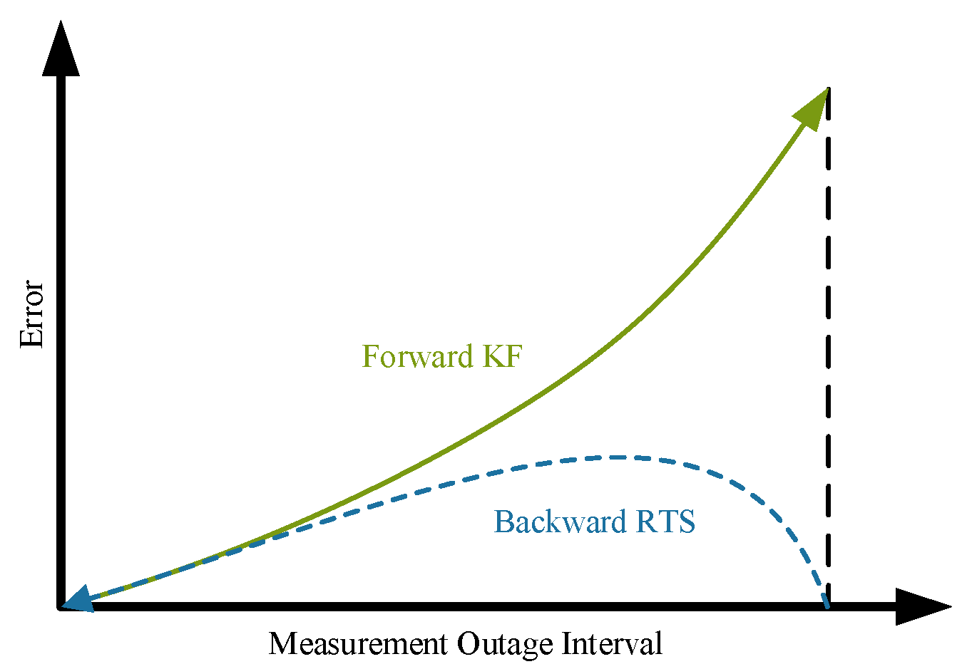
The intermittent corrections provided by ZUPT can cause abrupt changes in navigation information as the system transits from the swing phase to the stance phase. The RTS (Rauch–Tung–Striebel) optimal fixed-interval smoothing algorithm promises to mitigate such problem [26]. RTS smoothing can reduce estimation error effectively, and the error curve obtained by RTS smoothing is smoother than that obtained by Kalman Filtering, as shown in Figure 1.

The forward Kalman Filter process and the backward RTS process are taken here as an example. After the forward filtering is completed, RTS smoothing is carried out from time N to time 0 with initial values of ${\mathit{X}}_{N/N}^B=X_N^F$, ${\mathit{P}}_{N/N}^B=P_N^F$, and the update process is as follows:

$${\mathit{K}}_{k/N}^B={\mathit{P}}_k^F{\mathit{\Phi }}_{k+1,k}^T({\mathit{P}}_{k+1,k}^F{)}^{ - 1}$$

(26)

$${\mathit{X}}_{k/N}^B={\mathit{X}}_k^F+{\mathit{K}}_{k/N}^B({\mathit{X}}_{k+1/N}^B - {\mathit{X}}_{k+1,k}^F)$$

(27)

$${\mathit{P}}_{k/N}^B={\mathit{P}}_k^F+{\mathit{K}}_{k/N}^B({\mathit{P}}_{k+1/N}^B - {\mathit{P}}_{k+1,k}^F)({\mathit{K}}_{k/N}^B{)}^T$$

(28)

where the superscript F represents the variables of the forward filtering process, and the superscript B indicates the variables of the backward RTS process.

3.3. Forward–Backward Fusion

The Forward–Backward fusion framework utilizes the stored forward and backward navigation results and fuses them based on the covariance matrix of the Kalman Filter or the RTS smoothing algorithm. The idea is that the errors of both the forward and backward navigation accumulate over time, but the error accumulation processes of the two are opposite in time. Thus, at the same point in time, the forward and backward navigation errors exhibit different characteristics, as shown in Figure 2. Therefore, fusing the forward and backward navigation would yield better results.

Let the state vectors obtained from the forward and backward navigation processes be ${\mathit{X}}_1$ and ${\mathit{X}}_2$, with corresponding covariance matrices ${\mathit{P}}_1$ and ${\mathit{P}}_2$. Then, the fused state estimate of the Forward–Backward navigation would be the following linear combination of the state vectors:

$${\mathit{P}}_g=({\mathit{P}}_1^{ - 1}+{\mathit{P}}_2^{ - 1}{)}^{ - 1}$$

(29)

$${\mathit{X}}_g={\mathit{P}}_g\left({\mathit{P}}_1^{-1}{\mathit{X}}_1+{\mathit{P}}_2^{-1}{\mathit{X}}_2\right)$$

(30)

This fused state estimate can then be used to correct the navigation results. The corrected results are then used as reference values in the re-forward navigation process, yielding the final navigation results.

The proposed FB-RTS algorithm leverages the historical data already stored to optimize the navigation system. The architecture of the proposed FB-RTS algorithm is described in Figure 3. The two RTS modules operate in parallel rather than in a cascaded manner, ensuring its optimality by maintaining independence between forward and backward filtering processes. Song et al. demonstrated that when local estimators satisfy independence assumptions (e.g., uncorrelated process and measurement noises), their weighted fusion can achieve global optimality [27]. With the continuous advancements in computer technology, the processing power and storage capacity of computers and microcontrollers have seen significant improvements. This progress has made the implementation of the FB-RTS algorithm not only feasible but also cost-effective, with minimal additional expenditure.

4. Experimental Validation

To thoroughly evaluate the effectiveness of the proposed FB-RTS algorithm, this study employs a comprehensive validation approach encompassing both simulation experiments and two sets of field tests, both indoor and outdoor. The simulation experiments are designed to assess the algorithm’s capability to enhance navigation accuracy and mitigate heading drift during periods of motion, specifically in the absence of zero-velocity updates. Detailed error curves, especially velocity error curve, can then be examined, which is not easily obtainable in field tests. The indoor and outdoor field tests are designed to represent real-world complexities and evaluate the algorithm’s performance in terms of pedestrian localization accuracy and system reliability over extended periods and along comprehensive trajectories.

4.1. Experimental Overview

In this study, both field tests were conducted using self-developed wireless IMU sensor nodes, which are shown in Figure 4. Due to their relatively small size and low weight, they would not obstruct the normal gait of the subject. The IMU sensor employed in the sensor node was the ICM20948, which has been characterized through rigorous testing to provide the parameters shown in

Table 1. IMU error characteristics of the IMU sensor nodes used in field tests.

Sensor Type	White Noise	Bias Instability	Sampling Rate
Gyroscope	$0.5°/\sqrt{\mathrm{h}}$	$13°/\mathrm{h}$	$125 \mathrm{H}\mathrm{z}$
Accelerometer	$168\mu g/\sqrt{\mathrm{H}\mathrm{z}}$	$162 \mathsf{\mu }\mathrm{g}$	$125 \mathrm{H}\mathrm{z}$

:

These parameters ensure that the IMU sensor node delivers data that is representative of typical low-cost MIMU devices, suitable for validating the real-life potential of the proposed navigation algorithm.

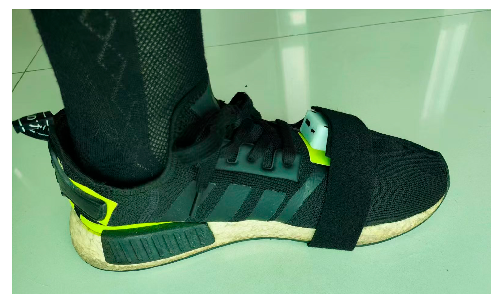
During field tests, a single IMU node is attached to the subjects’ feet using Velcro strap, specifically at the dorsal foot position. The IMU is oriented such that the y-axis roughly aligns with the direction of tiptoe, and the z-axis points approximately towards upward direction, as shown in Figure 5. The IMU is worn on the dorsal foot due to the known fact that it can mitigate the vibrations and acceleration peaks caused by heel strikes. The initial yaw angle of the SINS algorithm is set by minimizing the RMSE between the trajectory segment generated by the SINS algorithm (from the starting point to a point 3 m away) and the corresponding reference trajectory [28].

The FB-RTS algorithm operates in segments bounded by stance-phase midpoints, allowing the algorithm to operate in real time on a Lenovo laptop with AMD Ryzen 6800H processor, sourced in Nanjing, China. While optimized results for a segment incur ~13.7 ms latency post-segment, real-time forward navigation results are always available with ~0.05 ms latency using prior optimized states. For typical 160-sample segments (1.28 s), high-accuracy outputs are available within ~1.29 s.

To closely simulate real-world conditions, the IMU error characteristics in the simulation experiments are modeled to match the parameters shown in Table 1, along with a 10 mg accelerometer constant bias, allowing for a realistic simulation environment that can effectively mimic the behavior of the IMU sensor.

Alongside the proposed FB-RTS algorithm, the following three different algorithms are also carried out and compared. The ZUPT method is the baseline, representing the traditional solution detailed in Section 2, where no smoothing or segmentation is involved. The RTS method represents the proposed forward RTS smoothing solution implemented in a segmented fashion. The FB method represents the proposed Forward–Backward navigation solution implemented in a segmented fashion.

The effectiveness of the proposed FB-RTS algorithm will be preliminarily analyzed qualitatively using attitude, velocity, and position error curves. Quantitative analysis will be performed first by calculating the mean position error, maximum position error, and Root Mean Square Error (RMSE) of position for each algorithm. The RMSE of position is calculated using the following formula:

$$RMSE=\sqrt{{\displaystyle \frac{1}{N}}{\sum }_{i=1}^N{\left(x_i-{\widehat{x}}_i\right)}^2}$$

(31)

where $x_i$ is the true position, and ${\widehat{x}}_i$ is the estimated position at time i, with N being the total number of data points. Then, to provide a visual comparison of the algorithm’s performance and highlight the superiority of the proposed method, Cumulative Distribution Function (CDF) plots and distance percentage (D%) plots are introduced. The CDF curve illustrates the cumulative probability distribution of the position errors, while the D% curve represents the position error normalized by the distance traveled, providing a direct measure of the algorithm’s overall accuracy as the subject traverses along their trajectory.

4.2. Simulation Experiments

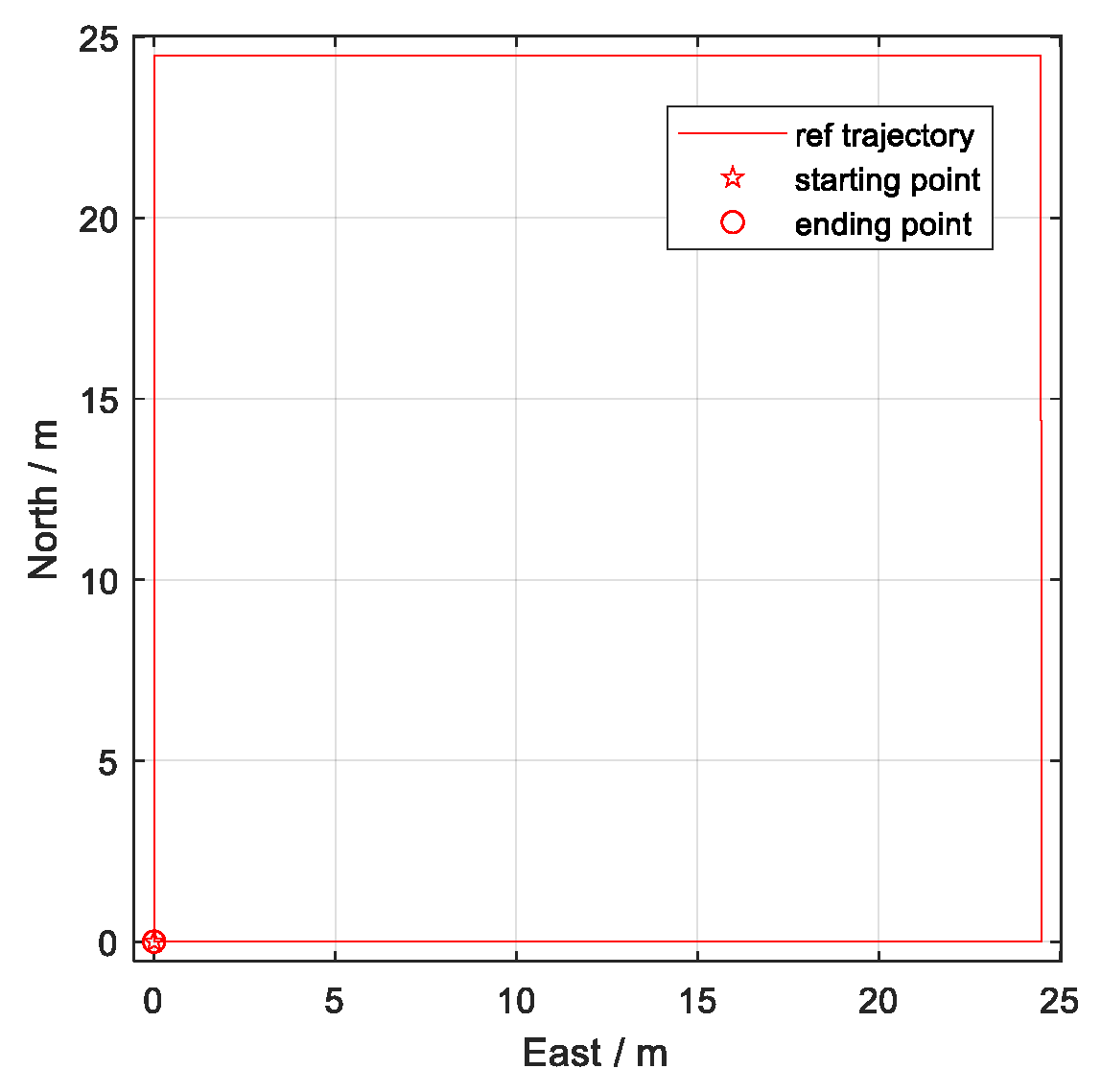
To effectively simulate the periodic zero-velocity characteristics of pedestrian walking, a simulated walking process is designed to replicate the cyclical process of “acceleration → deceleration → zero-velocity”. The simulated body moves along a square path in a clockwise direction, completing 8 laps, adding up to 783.36 m of total distance. Each phase of “acceleration → deceleration” and the “zero-velocity” phase lasts for 1 s, providing the algorithms with regular zero-velocity intervals. The ground truth trajectory and velocity for the simulation are detailed in Figure 6 and Figure 7. Note that $V_E$ and $V_U$ are consistently zero in Figure 7, thus the overlapping traces. Gyroscope constant bias was not added in simulation experiments, while bias instability was retained.

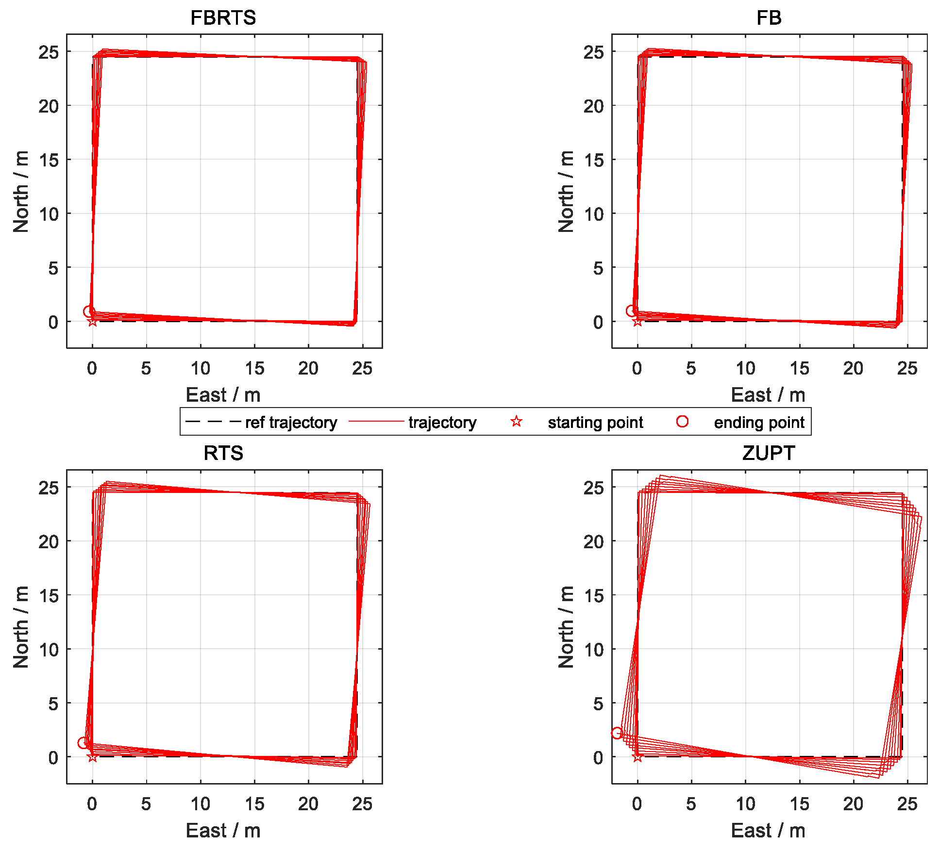
The trajectories resulting from the four algorithms are depicted in Figure 8, while Figure 9, Figure 10, Figure 11 and Figure 12 illustrates the attitude, velocity, and position error curves. As depicted in Figure 9, the heading divergence of the FB-RTS algorithm is significantly reduced compared to other algorithms, while the errors in pitch and roll remain the same. It is important to note that the error curves for pitch and roll are mainly attributed to the biases in the accelerometers, which are in fact exaggerated to mimic a worst-case scenario. Upon examining Figure 11, it is evident that the RTS algorithm provides a noticeable smoothing effect over the ZUPT algorithm; however, it does not significantly enhance absolute accuracy due to the fact that it uses only the forward filtering information. On the other hand, the FB algorithm, leveraging historical velocity and positional information, significantly reduces velocity error compared to ZUPT, thereby improving positional accuracy; however, its error curves still exhibit some randomness. The FB-RTS algorithm combines the advantages of both, with the smallest fluctuations and the smoothest error curves, clearly demonstrating the superiority of the proposed FB-RTS algorithm, which is further elaborated quantitatively in

Table 2. Error results of different algorithms in simulation experiments.

Algorithm	$\mathbf{Mean} \mathbf{Error}/\mathit{m}$	$\mathbf{RMSE}/\mathit{m}$	$\mathbf{Maximum} \mathbf{Error}/\mathit{m}$
ZUPT	1.07	1.32	2.94
RTS	0.596	0.723	1.64
FB	0.426	0.520	1.23
FB-RTS	0.362	0.460	1.19

.

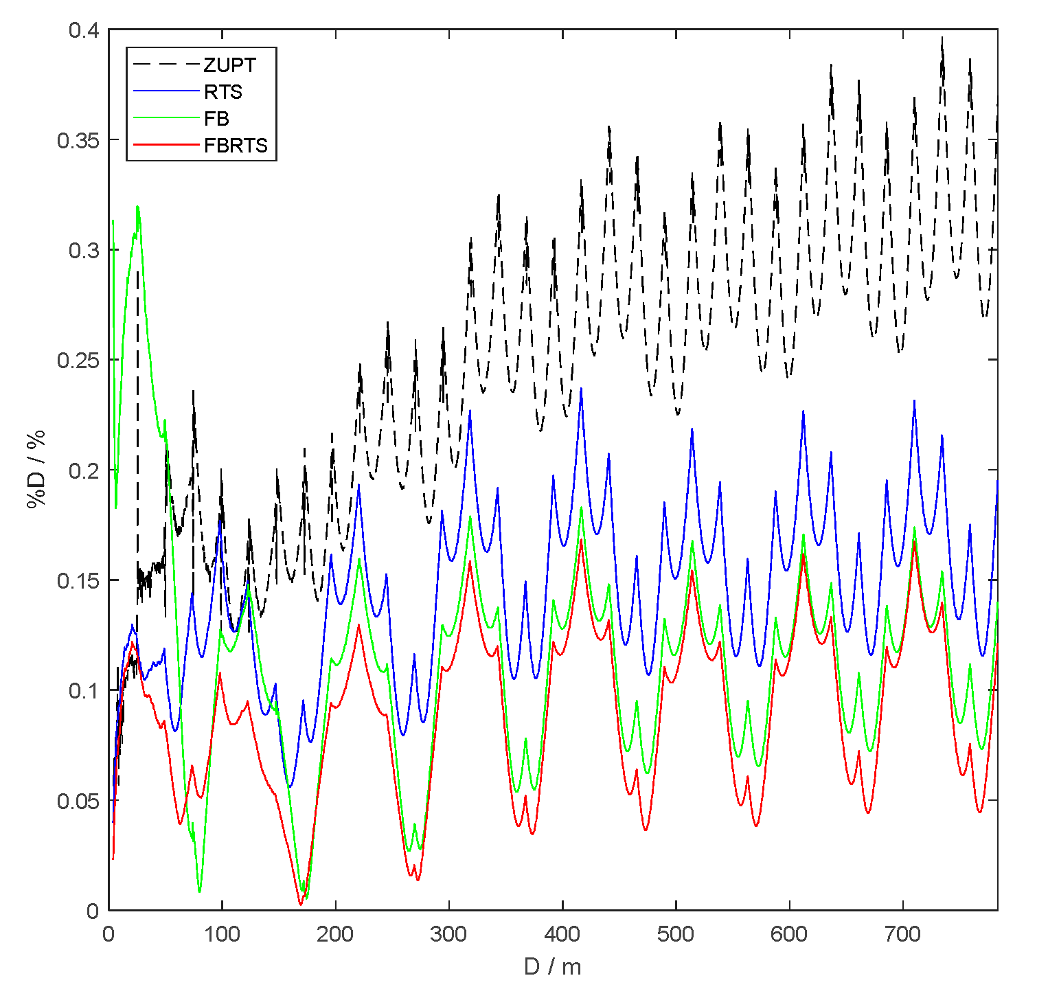
The CDF and D% plots for the four algorithms, as depicted in Figure 13 and Figure 14, provide a visual comparison of the positional accuracy across the tested methods. The error data and corresponding curves clearly demonstrate a hierarchy in precision, with FB-RTS outperforming FB, RTS, and at last ZUPT. It should be pointed out that the initial 150 m of the D% plot reveal that the performance of the four methods may not strictly adhere to the aforementioned ranking, particularly during the early stages of the walk. This observation suggests that while the proposed FB-RTS algorithm can mitigate the error accumulation process, its significant advantage over traditional methods becomes more pronounced over longer navigation periods. This characteristic aligns well with the practical demands and trends for pedestrian navigation, where long-duration and high-availability systems are increasingly sought after.

The simulation experiments have provided a controlled and systematic framework to evaluate the FB-RTS algorithm against existing methods. The results substantiate the FB-RTS algorithm’s enhanced performance in terms of error reduction and navigation accuracy. These findings pave the way for the following validation through real-world field tests.

4.3. Indoor Field Tests

Indoor field tests were conducted at the laboratory located in the Sipailou Campus of Southeast University, as shown in Figure 15. To obtain reliable ground truths for location reference, ten landmark points were marked at the intersection of the corridors by adhering paper markers to the ground, and the distances between these landmarks were calibrated using a laser rangefinder with an error parameter of ±3 mm. The resulting indoor map and the positions of the landmark points are depicted in Figure 16.

Prior to each experiment, gyroscope biases are estimated during a stationary initialization phase of 30 s and subtracted before operation [29]. A subject wore a single IMU node on their left foot and walked in straight lines between the landmark points. When arriving at a landmark point, the subject was instructed to roughly align their left foot with the marker and stand still for 2–3 s. This procedure allowed for accurate determination of when the IMU was positioned over the landmark point, ensuring that the actual position of the IMU node and the corresponding landmark point would not differ by more than a few centimeters.

Two sets of experiments were conducted, covering total distances of 308 m and 388 m, referred to as Path A and Path B, respectively. The trajectories resulting from the four algorithms are shown in Figure 17 and Figure 18, where the starting point of each trajectory is located at the origin (coordinates 0, 0). It can be observed that due to the discontinuity of the zero-velocity updates, the Kalman Filter states are prone to sudden changes when transitioning from the swing phase to the stance phase, leading to a jagged trajectory in the ZUPT algorithm, particularly prominent in the results of Path B. This significantly affects its navigation accuracy. In contrast, the other three methods exhibit smoother trajectories, although the FB algorithm also shows small non-smooth transitions, suggesting that applying RTS to FB can still improve navigation accuracy. Consistent with the observations from the simulation experiments, the proposed FB-RTS algorithm also demonstrates slightly improved heading accuracy over the other algorithms. This clearly showcases the superiority of the FB-RTS algorithm in real environments, which is quantitatively detailed in

Table 3. Error results of different algorithms in indoor field tests.

	Algorithm	$\mathbf{Mean} \mathbf{Error}/\mathit{m}$	$\mathbf{RMSE}/\mathit{m}$	$\mathbf{Maximum} \mathbf{Error}/\mathit{m}$
Path A	ZUPT	0.361	0.457	1.12
	RTS	0.319	0.389	0.858
	FB	0.285	0.323	0.560
	FB-RTS	0.272	0.301	0.472
Path B	ZUPT	0.788	0.942	2.24
	RTS	0.557	0.620	1.15
	FB	0.706	0.812	1.57
	FB-RTS	0.393	0.456	0.957

.

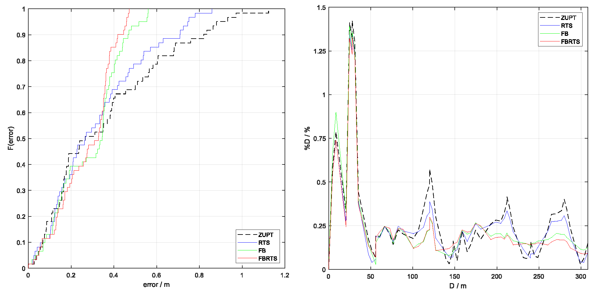
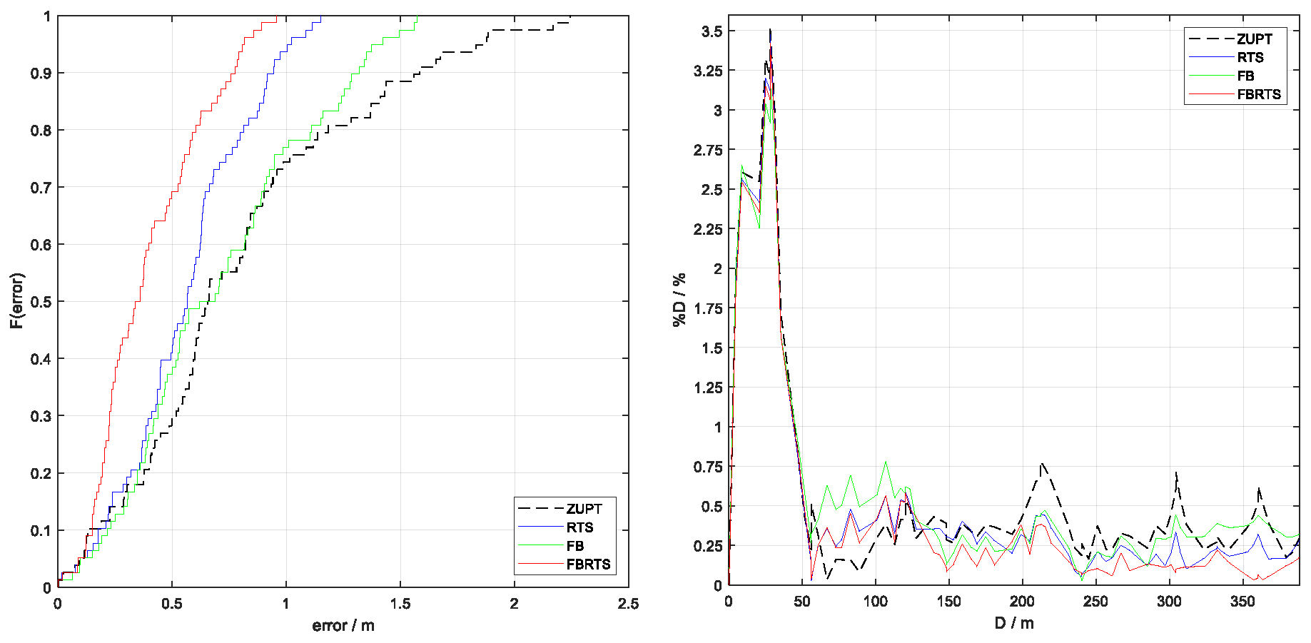
The CDF and D% plots for the four algorithms are presented in Figure 19 and Figure 20. It is evident that for both sets of experiments, the error data and curves indicate that the proposed FB-RTS performs the best, while the ZUPT, our baseline, performs the worst, with FB and RTS accuracies falling in between. Compared to ZUPT, the position RMSE of FB-RTS is improved by 34.1% and 51.6% in the two sets of experiments, respectively. However, the performance of FB and RTS is not consistent across the two experiments; for Path A, FB outperforms RTS, consistent with the simulation results, but for Path B, FB underperforms RTS. This discrepancy is due to variations in pedestrian gait or walking speed. Regardless, the FB-RTS algorithm significantly outperforms the traditional ZUPT algorithm in all experiments, while also demonstrating its superior robustness over the standalone application of FB or RTS.

Similarly to the findings from the simulation experiments, the initial 100 m of the D% plot reveal that the performance of the four methods does not necessarily align with the aforementioned precision ranking. This discrepancy can be attributed to the short accumulation time of errors, during which the differences among the algorithms are not pronounced. However, as the walking distance and duration increase, the advantages of the proposed FB-RTS method become more pronounced, and the D% curve becomes more stable than those of other algorithms. This observation underscores the effectiveness of the FB-RTS algorithm in mitigating error accumulation over longer navigation periods, thereby offering a more significant improvement in terms of robustness and high availability over traditional methods as the duration of navigation extends.

4.4. Outdoor Field Tests

Outdoor field tests were further conducted in the Sipailou Campus of Southeast University, aiming to provide long-distance evaluation of the proposed algorithm. To establish accurate ground truth for trajectory validation, a GNSS RTK (Real-Time Kinematic) setup was employed, providing centimeter-level positioning accuracy when RTK is enabled.

Prior to each experiment, IMU nodes underwent the same calibration and bias estimation procedures as in the indoor tests. A subject wore a single IMU node on their left foot and traversed two distinct paths, Path C and Path D, with a length of 2100 m and 2760 m, respectively. The subject was instructed to stop at locations with minimal GNSS signal obstruction for approximately 5 s. These stops served as reference points for evaluating the navigation accuracy of the algorithms. In total, 18 waypoints were recorded for Path C and 24 waypoints for Path D, distributed along the trajectories to ensure comprehensive coverage.

The trajectories generated by the four algorithms (ZUPT, RTS, FB, FB-RTS) are shown in Figure 21 and Figure 22, and their error results are detailed in

Table 4. Error results of different algorithms in outdoor field tests.

	Algorithm	$\mathbf{Mean} \mathbf{Error}/\mathit{m}$	$\mathbf{RMSE}/\mathit{m}$	$\mathbf{Maximum} \mathbf{Error}/\mathit{m}$
Path C	ZUPT	6.39	7.63	14.7
	RTS	5.54	7.00	16.1
	FB	5.25	6.14	12.4
	FB-RTS	4.98	5.62	8.80
Path D	ZUPT	6.31	7.92	15.0
	RTS	4.29	5.84	13.2
	FB	5.32	7.21	15.7
	FB-RTS	3.81	4.77	10.4

. The CDF and D% plots (Figure 23 and Figure 24) further confirmed the superiority of FB-RTS. For both paths, its position RMSE was 26.3% (Path C) and 39.8% (Path D) lower than ZUPT.

These results highlight the robustness of FB-RTS in long navigation sessions, further confirming the conclusions drawn from the indoor field tests. The algorithm’s ability to suppress error accumulation over multi-kilometer trajectories underscores its potential for real-world pedestrian navigation systems.

5. Discussion

A novel Forward–Backward navigation and RTS smoothing (FB-RTS) navigation scheme is proposed in this paper, designed to enhance the navigation accuracy of MIMU-based pedestrian navigation systems, without the need for additional sensors or specialized conditions. The FB-RTS algorithm harnesses the complete gait cycle of a pedestrian, utilizing historical data during both the stance and swing phases, to enhance navigation accuracy and reliability. First, both forward and backward integration method and the corresponding error equations are constructed, based on which the corresponding RTS smoother is applied. Second, both backward and forward RTS algorithms are established, where the system model and observation model are built under the output correction mode. Finally, both navigation results are combined to achieve the final estimation of attitude and velocity, where the position is recalculated by the optimized data.

Simulation experiments and two sets of field tests were conducted to validate the performance of the FB-RTS algorithm. The results demonstrated the algorithm’s superior performance in reducing navigation errors and smoothing pedestrian trajectories, offering a significant improvement over the traditional ZUPT method and both the FB and the RTS method. The FB-RTS algorithm’s ability to provide smoother and more accurate navigation trajectories was particularly evident in the real-world tests, offering a robust, adaptable and universal solution that is aligned with the growing demand for accurate and reliable indoor positioning technologies, well-suited for applications in smart buildings, wayfinding in complex indoor environments, and emergency response operations where precise indoor positioning is critical.