A Multi-Point Moment Matching Approach with Frequency-Aware ROM-Based Criteria for RLCk Model Order Reduction

Abstract

Model order reduction (MOR) is crucial for efficiently simulating large-scale RLCk models extracted from modern integrated circuits. Among MOR methods, balanced truncation offers strong theoretical error bounds but is computationally intensive and does not preserve passivity. In contrast, moment matching (MM) techniques are widely adopted in industrial tools due to their computational efficiency and ability to preserve passivity in RLCk models. Typically, MM approaches based on the rational Krylov subspace (RKS) are employed to produce reduced-order models (ROMs). However, the quality of the reduction is influenced by the selection of the number of moments and expansion points, which can be challenging to determine. This underlines the need for advanced strategies and reliable convergence criteria to adaptively control the reduction process and ensure accurate ROMs. This article introduces a frequency-aware multi-point MM (MPMM) method that adaptively constructs an RKS by closely monitoring the ROM transfer function. The proposed approach features automatic expansion point selection, local and global convergence criteria, and efficient implementation techniques. Compared to an established MM technique, MPMM achieves up to 16.3× smaller ROMs for the same accuracy, over 99.18% reduction in large-scale benchmarks, and up to 4× faster runtime. These advantages establish MPMM as a strong candidate for integration into industrial parasitic extraction tools.

1. Introduction

In recent years, advanced integrated circuit technologies, such as 3D packaging, have pushed the limits of performance and integration by overcoming key manufacturing limitations [1]. However, these advancements have introduced significant electromagnetic interactions, including mutual inductive coupling effects arising from densely packed interconnects and multi-layer routing structures. Modeling these interactions using parasitic extraction tools [2] often results in large-scale RLCk models with an extensive number of mutual inductances, rendering traditional SPICE simulation computationally intensive. Model order reduction (MOR) techniques aim to alleviate this issue by constructing reduced-order models (ROMs) that preserve the input–output behavior of the original systems, significantly reducing computational cost and simulation time.

MOR techniques can be classified into two main categories: balanced truncation (BT) and moment matching (MM). BT methods [3,4,5,6,7,8] provide robust approximation error bounds and can handle multi-port circuits effectively. However, BT becomes impractical for large-scale RLCk models as Gramian computation requires the solution of computationally expensive Lyapunov matrix equations and storage of dense matrices. Moreover, BT does not inherently preserve passivity [4] unless special post-processing techniques are applied, which often introduce additional computational overhead [3,9]. In contrast, MM methods [10,11,12,13,14,15,16,17] are better suited for large-scale model reduction due to their computational efficiency. These methods successfully exploit the sparsity of the system matrices and preserve passivity in symmetric RLCk systems by performing the projection through a congruence transformation [10]. However, the accuracy and size of the resulting ROM strongly depend on the quality of the underlying Krylov subspace.

MM techniques typically perform projection using the standard Krylov subspace [10], which is efficient at frequencies near the DC point but often degrades in accuracy at higher frequencies [16]. To overcome this limitation, the rational Krylov subspace (RKS) has been widely adopted in MOR methods [6,8,12,13,14,15,17]. Nevertheless, RKS performance heavily depends on the number and placement of the expansion points, which may be challenging to determine automatically. Although several methods use adaptive strategies or iteratively refine expansion points based on ROM quality, they still require the number of moments or the size of the ROM to be predefined [12,13,14,15,17]. Moreover, while most of them are suitable for ${\mathcal{H}}_2$-optimal reduction [6,12,13,17], offering globally optimal solutions, they often produce ROMs of unnecessarily high order in frequency-limited applications (e.g., circuit simulation). To improve ROM accuracy within specific frequency windows, authors in [14,15] propose using initial frequency bounds to guide the RKS construction. However, [14] requires the calculation of the original system transfer function, which is infeasible for large-scale models, while [15] selects expansion points based on the ROM dominant poles, a strategy that can overlook frequency regions with high approximation error. Furthermore, most methods often lack robust convergence criteria, which directly affects both ROM quality and reduction performance.

Beyond projection-based MOR techniques, data-driven methods for rational approximation have recently gained attention in the context of frequency-domain modeling. Algorithms such as AAA [18], Modified AAA [19], and AGORA [20] construct reduced-order rational approximations directly from frequency response samples, without access to the original system matrices. While these approaches are well-suited for small-scale or black-box systems, they are not directly applicable to large-scale RLCk models, where the sampling of the system’s frequency response can be computationally intensive.

These limitations highlight the need for frequency-aware MOR methods with reliable convergence criteria, which can adaptively refine the RKS in regions of high approximation error. In this work, we propose a frequency-aware multi-point MM (MPMM) method that iteratively builds an RKS, guided by the ROM transfer function error. The proposed method adaptively selects expansion points and assesses convergence based on local and global convergence criteria, ensuring compact and accurate ROMs over the frequency range of interest. Building upon our prior methodology for low-rank BT via multi-point RKS projection [8], this work extends the concept to MM and introduces the following key contributions:

• Two discrete convergence criteria, entirely based on the ROM’s transfer function, avoiding the calculation of the original model’s response [14]. The local convergence criterion allows the number of moments per expansion point to be chosen automatically, eliminating the need for fixed iteration counts [15], while the global convergence criterion provides a reliable assessment of the overall ROM accuracy.
• An adaptive expansion point selection strategy, where each subsequent expansion point is selected based on the current ROM error profile. This allows the algorithm to target the most critical frequency regions.
• Efficient implementation techniques, such as sparse/dense matrix handling and substitution of matrix inversions by linear solves, enabling fast and scalable reduction of large-scale RLCk models.

An extensive evaluation against an established MM method [15] demonstrates that MPMM produces ROMs that are 2.6× on average and up to 16.3× smaller for the same accuracy, achieving over 99.18% order reduction for large-scale models. Additionally, it exhibits up to 4× faster reduction time, with an average speedup of 2.3×, and up to 2.5× less memory consumption, further highlighting its computational efficiency. Given its effectiveness, the proposed method can be integrated into industrial parasitic extraction tools, such as ANSYS RaptorH™ [2], enabling an efficient reduction in complex RLCk circuit models.

The remainder of this article is organized as follows. Section 2 provides a review of existing MOR techniques, focusing on MM methods. Section 3 outlines the key concepts of MM and introduces the RKS. Section 4 presents our proposed MPMM methodology along with efficient implementation techniques. Section 5 reports the experimental results, and Section 6 concludes this article.

2. Related Work

MOR has been a key enabler for efficiently simulating large-scale RLCk models of integrated circuits. Among various MOR techniques [3,4,5,6,7,8,10,11,12,13,14,15,16,17], two main families have been widely explored: MM and BT. BT methods [3,4,5,6,7,8] provide theoretical error bounds and strong control over the approximation quality. They achieve model reduction by solving large-scale Lyapunov equations and performing a balancing transformation based on the controllability and observability Gramians of the system. However, applying BT directly to large models is often infeasible due to the high computational and memory costs of solving dense matrix equations, even with low-rank approximations. Moreover, BT does not guarantee passivity unless post-reduction passivity enforcement techniques [3,9] are applied, further increasing computational cost. On the other hand, MM approaches [10,11,12,13,14,15,16,17] have been widely used in industrial tools [2] due to their simplicity and robustness. MM techniques generate ROMs by projecting the original system onto Krylov subspaces, effectively matching the moments of the original system’s transfer function around selected expansion points. Such methods inherently preserve passivity for symmetric RLCk systems [10] and are highly scalable for large-scale, sparse descriptor models.

Traditional MM approaches use the standard Krylov subspace, where the basis is generated around the DC expansion point [10,11]. Although such methods have straightforward implementation and are computationally efficient, their accuracy is localized around the DC frequency and degrades rapidly for frequencies farther away. To improve approximation quality, the extended Krylov subspace (EKS) has been proposed [16,17]. EKS combines the standard and inverse Krylov subspaces, expanding the subspace both around DC and infinity, improving spectral coverage from low to high frequencies in a single projection. However, like their predecessors, EKS-based methods struggle to maintain high accuracy in specific frequencies, as they target the entire frequency spectrum [6].

To address this limitation, RKS-based methods [6,12,13,14,15,17] further generalize MM by introducing arbitrary real or complex shifts in the projection process. In the context of circuit simulation, using real shifts is preferred to maintain real-valued ROMs [15]. Several techniques based on RKS aim to achieve ${\mathcal{H}}_2$-optimality [6,12,13,17]. The well-known IRKA algorithm [12] attempts to minimize the system’s ${\mathcal{H}}_2$-norm error by approximating the eigenvalues of the original system given a fixed ROM order r. This is performed through an iterative refinement of the shift parameters for the RKS. However, it requires a repeated calculation of the ROM eigenvalues and reconstruction of the RKS, which reduces its applicability to large-scale problems. The authors of [6,13] proposed more flexible versions of IRKA, which initially construct an RKS and then adaptively select subsequent expansion points based on ROM eigenvalues to expand the subspace, aiming to reduce computational cost. More advanced approaches have introduced a combination of EKS and RKS [17], achieving better results. Nevertheless, these methods [6,12,13,17] often produce unnecessarily large ROMs when only a limited frequency band is of interest.

To improve efficiency in frequency-limited applications, multi-point RKS methods have been developed [14,15]. The method proposed in [15] employs an adaptive three-point selection strategy (A3PSA), which selects expansion points at low, mid, and high frequencies based on a user-defined frequency range and the dominant poles of the system, following the IRKA scheme [12]. ROM accuracy is assessed by considering the differences in ROM eigenvalues computed at the previous and current three points (low, mid, and high). However, this technique assumes a fixed number of matched moments per expansion point, which may lead to suboptimal ROM sizes. The fully adaptive scheme presented in [14] dynamically selects expansion points based on the frequency at which the error between the transfer function of the original model and the ROM is the largest. The number of moments is then adjusted by monitoring the error within the interval between neighboring expansion points. Despite being promising, this method relies on a repeated evaluation of the original model’s response, which is practically infeasible for large-scale models.

Contrary to existing multi-point approaches [14,15], the proposed method relies exclusively on ROM-level information to guide both the selection of expansion points and the construction of the RKS. Moreover, the addition of a local convergence criterion allows the number of moments per expansion point to be determined automatically, avoiding unnecessary computations. Finally, our method can benefit from less frequent convergence checks, further improving reduction time.

3. MOR by MM

Using the modified nodal analysis (MNA) [21], a linear RLCk circuit with n nodes, m (inductive) branches, p inputs, and q outputs can be described in the time domain as

$$\begin{array}{c}\left(\begin{array}{cc}{\mathbf{G}}_n& \mathbf{E}\\ {\mathbf{E}}^T& \mathbf{0}\end{array}\right)\left(\begin{array}{c}\mathbf{v}\left(t\right)\\ \mathbf{i}\left(t\right)\end{array}\right)+\left(\begin{array}{cc}{\mathbf{C}}_n& \mathbf{0}\\ \mathbf{0}& -\mathbf{M}\end{array}\right)\left(\begin{array}{c}\dot{\mathbf{v}}\left(t\right)\\ \dot{\mathbf{i}}\left(t\right)\end{array}\right)=\left(\begin{array}{c}{\mathbf{B}}_1\\ \mathbf{0}\end{array}\right)\mathbf{u}\left(t\right),\\ \mathbf{y}\left(t\right)=\left(\begin{array}{c}{\mathbf{L}}_1\mathbf{0}\end{array}\right)\left(\begin{array}{c}\mathbf{v}\left(t\right)\\ \mathbf{i}\left(t\right)\end{array}\right),\end{array}$$

(1)

where ${\mathbf{G}}_n\in {\mathbb{R}}^{n\times n}$ is the node conductance matrix, ${\mathbf{C}}_n\in {\mathbb{R}}^{n\times n}$ is the node capacitance matrix, $\mathbf{M}\in {\mathbb{R}}^{m\times m}$ is the branch inductance matrix, $\mathbf{E}\in {\mathbb{R}}^{n\times m}$ is the node-to-branch incidence matrix, $\mathbf{v}\in {\mathbb{R}}^n$ is the vector of node voltages, $\mathbf{i}\in {\mathbb{R}}^m$ is the vector of inductive branch currents, $\mathbf{u}\in {\mathbb{R}}^p$ is the vector of input excitations, ${\mathbf{B}}_1\in {\mathbb{R}}^{n\times p}$ is the input-to-node connectivity matrix, $\mathbf{y}\in {\mathbb{R}}^q$ is the vector of output measurements, and ${\mathbf{L}}_1\in {\mathbb{R}}^{q\times n}$ is the node-to-output connectivity matrix. Moreover, we consider $\dot{\mathbf{v}}\left(t\right)\equiv {\displaystyle \frac{d\mathbf{v}\left(t\right)}{dt}}$ and $\dot{\mathbf{i}}\left(t\right)\equiv {\displaystyle \frac{d\mathbf{i}\left(t\right)}{dt}}$. By defining the model order as $N\equiv n+m$, the state vector as $\mathbf{x}\left(t\right)\equiv \left(\begin{array}{c}\mathbf{v}\left(t\right)\\ \mathbf{i}\left(t\right)\end{array}\right)$, and also

$$\begin{array}{c}\mathbf{G}\equiv -\left(\begin{array}{cc}{\mathbf{G}}_n& \mathbf{E}\\ {\mathbf{E}}^T& \mathbf{0}\end{array}\right),\mathbf{C}\equiv \left(\begin{array}{cc}{\mathbf{C}}_n& \mathbf{0}\\ \mathbf{0}& -\mathbf{M}\end{array}\right),\mathbf{B}\equiv \left(\begin{array}{c}{\mathbf{B}}_1\\ \mathbf{0}\end{array}\right),\mathbf{L}\equiv \left(\begin{array}{c}{\mathbf{L}}_1\mathbf{0}\end{array}\right),\end{array}$$

(2)

the descriptor form is obtained:

$$\mathbf{C}{\displaystyle \frac{d\mathbf{x}\left(t\right)}{dt}}=\mathbf{Gx}\left(t\right)+\mathbf{Bu}\left(t\right),\mathbf{y}\left(t\right)=\mathbf{Lx}\left(t\right).$$

(3)

The primary goal of MOR is to compute a ROM:

$$\tilde{\mathbf{C}}{\displaystyle \frac{d\tilde{\mathbf{x}}\left(t\right)}{dt}}=\tilde{\mathbf{G}}\tilde{\mathbf{x}}\left(t\right)+\tilde{\mathbf{B}}\mathbf{u}\left(\mathbf{t}\right),\tilde{\mathbf{y}}\left(t\right)=\tilde{\mathbf{L}}\tilde{\mathbf{x}}\left(t\right),$$

where $\tilde{\mathbf{G}},\tilde{\mathbf{C}}\in {\mathbb{R}}^{r\times r}$, $\tilde{\mathbf{B}}\in {\mathbb{R}}^{r\times p}$, $\tilde{\mathbf{L}}\in {\mathbb{R}}^{q\times r}$, with $r<<N$, such that the ROM accurately approximates the original system. The approximation quality is measured by the output error, which is bounded in the time domain as

$$\left|\right|\tilde{\mathbf{y}}\left(t\right)-{\mathbf{y}\left(t\right)\left|\right|}_2{<\epsilon \left|\right|\mathbf{u}\left(t\right)\left|\right|}_2,$$

for any input $\mathbf{u}\left(t\right)$ and a small tolerance $\epsilon$. Using Plancherel’s theorem [22], the error bound can be equivalently expressed in the frequency domain as

$$\left|\right|\tilde{\mathbf{y}}\left(s\right)-{\mathbf{y}\left(s\right)\left|\right|}_2{<\epsilon \left|\right|\mathbf{u}\left(s\right)\left|\right|}_2.$$

Let $\mathbf{H}\left(s\right)$ and $\tilde{\mathbf{H}}\left(s\right)$ denote the transfer functions of the original model and the ROM, respectively:

$$\mathbf{H}\left(s\right)=\mathbf{L}{(s\mathbf{C}-\mathbf{G})}^{-1}\mathbf{B},\tilde{\mathbf{H}}\left(s\right)=\tilde{\mathbf{L}}{(s\tilde{\mathbf{C}}-\tilde{\mathbf{G}})}^{-1}\tilde{\mathbf{B}}.$$

(4)

Then, the output error in the frequency domain satisfies:

$$\left|\right|\tilde{\mathbf{y}}\left(s\right)-{\mathbf{y}\left(s\right)\left|\right|}_2=\left|\right|\tilde{\mathbf{H}}\left(s\right)\mathbf{u}\left(s\right)-{\mathbf{H}\left(s\right)\mathbf{u}\left(s\right)\left|\right|}_2\le \left|\right|\tilde{\mathbf{H}}\left(s\right)-{\mathbf{H}\left(s\right)\left|\right|}_{\infty }{\left|\right|\mathbf{u}\left(s\right)\left|\right|}_2,$$

where ${\left|\right|.\left|\right|}_{\infty }$ denotes the ${\mathcal{H}}_{\infty }$ norm of a rational transfer function. Therefore, ensuring that $\left|\right|\tilde{\mathbf{H}}\left(s\right)-\mathbf{H}\left(s\right){\left|\right|}_{\infty }<\epsilon$, guarantees that the ROM accurately approximates the behavior of the original system for any input excitation.

MM provides an efficient way for reducing linear systems, being particularly useful for circuit simulation and descriptor models. Starting from the time-domain descriptor system (Equation (3)), the application of the Laplace transform yields the following frequency-domain representation:

$$s\mathbf{C}\mathbf{x}\left(s\right)-\mathbf{x}\left(0\right)=\mathbf{G}\mathbf{x}\left(s\right)+\mathbf{B}\mathbf{u}\left(s\right),\mathbf{y}\left(s\right)=\mathbf{L}\mathbf{x}\left(s\right).$$

If we now assume zero initial conditions (i.e., $\mathbf{x}\left(s\right)=0$ and $\mathbf{u}\left(s\right)=1$), then the above system can be written as

$$(s\mathbf{C}-\mathbf{G})\mathbf{x}\left(s\right)=\mathbf{B},\mathbf{y}\left(s\right)=\mathbf{L}\mathbf{x}\left(s\right).$$

Expanding the original system’s transfer function $\mathbf{H}\left(s\right)$ as a Taylor series around an expansion point $s_0$ (commonly $s_0=0$) gives

$$\mathbf{H}\left(s\right)={\mathbf{M}}_0+{\mathbf{M}}_1(s-s_0)+{\mathbf{M}}_2{(s-s_0)}^2+\dots ,$$

where the coefficients ${\mathbf{M}}_k$ are the system’s moments at $s_0$. In particular, for circuit models, ${\mathbf{M}}_0$ corresponds to the DC behavior, where inductors are treated as short circuits and capacitors as open circuits, whereas ${\mathbf{M}}_1$ captures the system’s dominant time constant, characterizing its response to external inputs. In general, these block moments can be calculated using the following relation:

$${\mathbf{M}}_k={\mathbf{L}}^T{\left({\mathbf{G}}^{-1}\mathbf{C}\right)}^k{\mathbf{G}}^{-1}\mathbf{B}.$$

The key idea of MM is to construct a ROM, such that its transfer function matches several moments of the original system’s transfer function around selected frequency points. This is achieved via projection onto a lower-dimensional subspace. Let ${\mathbf{V}}_r,{\mathbf{V}}_l\in {\mathbb{R}}^{N\times r}$ denote the right and left projection matrices, respectively. For an expansion around $s_0=0$, the subspaces that these projection matrices span are

$$\begin{array}{c}range\left({\mathbf{V}}_r\right)=span\{{\mathbf{G}}^{-1}\mathbf{B},\left({\mathbf{G}}^{-1}\mathbf{C}\right){\mathbf{G}}^{-1}\mathbf{B},\dots ,{\left({\mathbf{G}}^{-1}\mathbf{C}\right)}^{r-1}{\mathbf{G}}^{-1}\mathbf{B}\},\\ range\left({\mathbf{V}}_l\right)=span\{{\mathbf{L}}^T,\left({\mathbf{C}}^T{\mathbf{G}}^{-T}\right){\mathbf{L}}^T,\dots ,{\left({\mathbf{C}}^T{\mathbf{G}}^{-T}\right)}^{r-1}{\mathbf{L}}^T\}.\end{array}$$

By projecting the original system matrices, the ROM is formed as

$$\tilde{\mathbf{C}}={\mathbf{V}}_l^T\mathbf{C}{\mathbf{V}}_r,\tilde{\mathbf{G}}={\mathbf{V}}_l^T\mathbf{G}{\mathbf{V}}_r,\tilde{\mathbf{B}}={\mathbf{V}}_l^T\mathbf{B},\tilde{\mathbf{L}}=\mathbf{L}{\mathbf{V}}_r.$$

The resulting ROM transfer function $\tilde{\mathbf{H}}\left(s\right)$ matches the first $2r$ moments of the original transfer function $\mathbf{H}\left(s\right)$.

Typically, the projection subspaces are constructed using Krylov sequences based on the system matrices. In the case of symmetric systems, a single-sided projection can be employed (i.e., ${\mathbf{V}}_l={\mathbf{V}}_r$), enabling efficient reduction in large-scale models while inherently preserving ROM passivity [10]. Typical MM techniques based on the standard Krylov subspaces offer excellent efficiency near the DC point. However, their accuracy degrades at higher frequencies, limiting their applicability to broadband or frequency-selective problems [16].

To address this issue, RKS-based projection techniques have been developed, incorporating multiple expansion points to improve approximation quality across wider frequency ranges. If we define $\mathbf{G}\left(s_i\right)\equiv \mathbf{G}+s_i\mathbf{C}$ and also $\mathbf{A}\left(s_i\right)\equiv -\mathbf{G}{\left(s_i\right)}^{-1}\mathbf{C}$, $\mathbf{F}\left(s_i\right)\equiv \mathbf{G}{\left(s_i\right)}^{-1}\mathbf{B}$, then the RKS of order j associated with the matrix pair ($\mathbf{A},\mathbf{F}$) and a set of expansion points $\mathbf{s}=\{s_1,s_2,\dots ,s_j\}$ is defined as

$${\mathcal{K}}_k^R(\mathbf{A},\mathbf{F},\mathbf{s})=span\{\mathbf{A}\left(s_1\right)\mathbf{F}\left(s_1\right),\mathbf{A}\left(s_2\right)\mathbf{F}\left(s_2\right),\dots ,\prod _{i=1}^j\mathbf{A}\left(s_i\right)\mathbf{F}\left(s_i\right)\}.$$

By appropriately choosing the shifts, the ROM can accurately capture the system dynamics over a targeted frequency band. Nevertheless, the selection of expansion points and the number of matched moments remain critical for ensuring good accuracy. Poor choice of expansion points can lead to reduced accuracy at frequencies that are not well represented by the matched moments.

4. Proposed Methodology

This section presents our multi-point MM (MPMM) framework based on RKS for accurately reducing large-scale RLCk models. The methodology adaptively builds the RKS by selecting frequency points where the ROM approximation error is maximized, ensuring accurate coverage across the frequency range of interest. At each step, the algorithm constructs a ROM via projection, monitors convergence through reliable local and global error indicators, and dynamically selects the expansion points. The proposed MPMM procedure is presented in Algorithm 1.

Algorithm 1 Proposed multi-point MM (MPMM) method

Inputs: $\mathbf{G},\mathbf{C},\mathbf{B},\mathbf{L},\mathbf{s}$ Outputs: $\tilde{\mathbf{G}},\tilde{\mathbf{C}},\tilde{\mathbf{B}},\tilde{\mathbf{L}}$   1: ${\mathbf{s}}_{used}=\left[\right]$; $s_k=get\_next\_frequency(\mathbf{s},{\mathbf{s}}_{used})$   2: ${\mathbf{K}}^{\left(j\right)}=\left[\right]$;   3: while ${\mathbf{s}}_{used}\ne \mathbf{s}$ do   4:     ${\mathbf{s}}_{used}=[{\mathbf{s}}_{used},s_k]$   5:     ${\mathbf{K}}^{\left(j\right)}=[{\mathbf{K}}^{\left(j\right)},Orth\left(\mathbf{F}\left(s_k\right)\right)]$   6:     $j=1$; $p=col\_size\left(\mathbf{B}\right)$; $k=col\_size\left({\mathbf{K}}^{\left(j\right)}\right)$   7:     while $j<max\_local\_iters$ do   8:         Calculate ROM: $\tilde{\mathbf{C}}={\mathbf{K}}^{\left(j\right)T}\mathbf{C}{\mathbf{K}}^{\left(j\right)},\tilde{\mathbf{G}}={\mathbf{K}}^{\left(j\right)T}\mathbf{G}{\mathbf{K}}^{\left(j\right)},\tilde{\mathbf{B}}={\mathbf{K}}^{\left(j\right)T}\mathbf{B},\tilde{\mathbf{L}}=\mathbf{L}{\mathbf{K}}^{\left(j\right)}$   9:         if $global\_error\left(\right)<global\_tol$ return 10:         if $local\_error\left(\right)<local\_tol$ break 11:         ${\mathbf{K}}_1=\mathbf{A}\left(s_k\right){\mathbf{K}}^{\left(j\right)}(:,k-p:k)$ 12:         ${\mathbf{K}}_2=Orth\left({\mathbf{K}}_1\right)$    w.r.t.    ${\mathbf{K}}^{\left(j\right)}$ 13:         ${\mathbf{K}}_3=Orth\left({\mathbf{K}}_2\right)$ 14:         ${\mathbf{K}}^{(j+1)}=[{\mathbf{K}}^{\left(j\right)},{\mathbf{K}}_3]$    15:         $j=j+1$; $k=k+p$ 16:     end while 17:     $s_k=get\_next\_frequency(\mathbf{s},{\mathbf{s}}_{used})$ 18: end while

Algorithm 1 receives as input the MNA matrices of the original model ($\mathbf{G},\mathbf{C},\mathbf{B},\mathbf{L}$), as defined in Equation (2), along with a predefined set $\mathbf{s}$ of $freq\_points\_num$ candidate expansion points covering the desired frequency range. The output consists of the ROM matrices ($\tilde{\mathbf{G}},\tilde{\mathbf{C}},\tilde{\mathbf{B}},\tilde{\mathbf{L}}$). The reduction process is adaptive and driven by effective two convergence criteria, detailed in Section 4.2. The local convergence criterion ensures sufficient moment matching at each selected frequency point, while the global convergence criterion verifies that the ROM achieves the required accuracy across the entire frequency range. Expansion points (${\mathbf{s}}_{used}$) are dynamically selected from the candidate set $\mathbf{s}$ following the strategy described in Section 4.3. For each expansion point $s_k$, the initial basis vectors are computed in step 5 as $\mathbf{F}\left(s_k\right)$. In steps 7–16, subsequent vectors are generated iteratively, forming a local RKS of dimension j:

$${\mathcal{K}}_j^{s_k}(\mathbf{A},\mathbf{F},s_k)=span\{\mathbf{F}\left(s_k\right),\mathbf{A}\left(s_k\right)\mathbf{F}\left(s_k\right),\mathbf{A}{\left(s_k\right)}^2\mathbf{F}\left(s_k\right),\dots ,\mathbf{A}{\left(s_k\right)}^{j-1}\mathbf{F}\left(s_k\right)\}.$$

The expansion at $s_k$ continues until the local convergence criterion is satisfied, indicating that a further addition of moments at this frequency point is unnecessary. Upon reaching local convergence, a new expansion point is selected from the remaining candidates in step 17. This iterative procedure continues until the global convergence criterion is met. The final RKS is the combination of subspaces constructed around all selected expansion points ${\mathbf{s}}_{used}$, as depicted in Figure 1:

$$\begin{array}{c}\hfill {\mathcal{K}}_j^{{\mathbf{s}}_{used}}(\mathbf{A},\mathbf{F},{\mathbf{s}}_{used})=span\{\mathbf{F}\left(s_1\right),\mathbf{A}\left(s_1\right)\mathbf{F}\left(s_1\right),\dots ,\mathbf{A}{\left(s_1\right)}^{j_1-1}\mathbf{F}\left(s_1\right),\dots ,\\ \hfill \mathbf{F}\left(s_{\nu }\right),\mathbf{A}\left(s_{\nu }\right)\mathbf{F}\left(s_{\nu }\right),\dots ,\mathbf{A}{\left(s_{\nu }\right)}^{j_{\nu }-1}\mathbf{F}\left(s_{\nu }\right)\},\end{array}$$

where $\nu$ is the total number of used expansion points (${\mathbf{s}}_{used}$) and $j_k$ denotes the number of iterations performed at each point $s_k$.

4.1. Orthogonalization Process

The orthogonalization steps in Algorithm 1 ($Orth$) are performed using a modified Gram–Schmidt procedure [23]. In step 12, orthogonalization with respect to ${\mathbf{K}}^{\left(j\right)}$ follows a block-wise procedure:

for$\zeta =1:2$do     for$k_1=1:k/p$do         $k_2=p(k_1-1)$; $k_3=k2+p$         ${\mathbf{K}}_2={\mathbf{K}}_1-{\mathbf{K}}^{\left(j\right)}(:,k_2+1:k_3){\mathbf{K}}^{\left(j\right)T}(:,k_2+1:k_3){\mathbf{K}}_1$     end for end for

This ensures that the RKS vectors remain linearly independent and well conditioned.

4.2. Convergence Criteria

Convergence in steps 9–10 is evaluated periodically every $convergence\_period$ iterations, rather than at every iteration, to reduce computational overhead. The ROM transfer function $\tilde{\mathbf{H}}\left(s\right)$ is used to monitor both global and local convergence. The error at iteration j is defined as

$$\underset{i=1\dots l}{max}{\displaystyle \frac{\left|\right|{\tilde{\mathbf{H}}}_j\left(s_i\right)-{\tilde{\mathbf{H}}}_{j-1}\left(s_i\right){\left|\right|}_{\infty }}{\left|\right|{\tilde{\mathbf{H}}}_j\left(s_i\right){\left|\right|}_{\infty }}},$$

where ${\tilde{\mathbf{H}}}_j\left(s_i\right)$ is the ROM transfer function at the j-th iteration (calculated using the expansion point $s_i$) and l is the number of evaluation points.

• Global convergence evaluates the ROM transfer function over the entire candidate set of expansion points $\mathbf{s}$ to ensure uniform accuracy across the desired frequency range.
• Local convergence focuses on the current expansion point ($s_k$) and its neighboring points ($0.85\ast s_k,0.95\ast s_k,1.05\ast s_k,1.15\ast s_k$) to ensure accurate local approximation around $s_k$.

4.3. Expansion Point Selection

The candidate expansion points $\mathbf{s}$ are selected based on one of two strategies:

• Uniform distribution: Expansion points are evenly distributed within a user-defined frequency range.
• User-defined frequencies: Expansion points are specified directly by the user according to targeted frequency bands.

The dynamic selection of each expansion point $s_k$ in Algorithm 1 ($get\_next\_frequency$) follows these rules:

• The first point is chosen as the lowest frequency in $\mathbf{s}$ (step 1).
• The second point is selected as the highest frequency.
• Subsequent points are chosen based on the maximum global approximation error among unused candidate expansion points.

This strategy prioritizes refining the ROM at the frequencies where the current ROM exhibits the largest error.

A critical aspect of Krylov subspace projection is deciding whether to use real, imaginary, or complex expansion points. When constructing the RKS, only real expansion points are employed for the following reasons [24]:

• The MNA matrices of the original model (Equation (2)) are real; using complex shifts would introduce complex arithmetic, increasing computational cost [15].
• Real shifts offer broader convergence across the frequency spectrum, while imaginary shifts, despite their excellent local accuracy, may degrade performance away from the interpolation point [11].

4.4. Efficient Implementation Details

Several efficient implementation strategies are applied to ensure high MPMM performance and scalability.

4.4.1. Matrix Inversions as Linear Solves

Algorithm 1 involves the direct inversion of matrix $(\mathbf{G}+s_k\mathbf{C})$, which is computationally prohibitive and can be effectively avoided. Since this matrix is only needed in matrix products with p vectors in steps 5 and 11, the matrix products involving inverse matrices are computed by equivalently solving the sparse linear system:

$$\mathbf{Y}={(\mathbf{G}+s_k\mathbf{C})}^{-1}\mathbf{B}\iff (\mathbf{G}+s_k\mathbf{C})\mathbf{Y}=\mathbf{B}.$$

This approach avoids dense inversions and preserves the sparsity of the system matrices.

4.4.2. Handling of Sparse/Dense Sub-Matrices

The matrix $\mathbf{C}$ of Equation (2) contains a sparse block ${\mathbf{C}}_n$ and a dense block $\mathbf{M}$ due to the mutual inductance couplings. Therefore, for optimal handling, the sparse sub-matrix ${\mathbf{C}}_n$ and the dense sub-matrix $\mathbf{M}$ within $\mathbf{C}$ are handled separately. The operation $-(\mathbf{G}+s_k\mathbf{C})\mathbf{Y}=\mathbf{V}$ can be represented as a $2\times 2$ block system of equations:

$$\begin{array}{c}\left(\begin{array}{c}-\left(\begin{array}{cc}{\mathbf{G}}_n& \mathbf{E}\\ {\mathbf{E}}^T& \mathbf{0}\end{array}\right)-s_k\left(\begin{array}{cc}{\mathbf{C}}_n& \mathbf{0}\\ \mathbf{0}& -\mathbf{M}\end{array}\right)\end{array}\right)\left(\begin{array}{c}{\mathbf{Y}}_u\\ {\mathbf{Y}}_l\end{array}\right)=\left(\begin{array}{c}{\mathbf{V}}_u\\ {\mathbf{V}}_l\end{array}\right)\hfill \\ \hfill \hspace{1em}\hspace{1em}\hspace{1em}\hspace{1em}\hspace{1em}\hspace{1em}\hspace{1em}\hspace{1em}\hspace{1em}\hspace{1em}\hspace{1em}\hspace{1em}\hspace{1em}\hspace{1em}\hspace{1em}\iff \left(\begin{array}{cc}{\mathbf{G}}_n+s_k{\mathbf{C}}_n& \mathbf{E}\\ {\mathbf{E}}^T& -s_k\mathbf{M}\end{array}\right)\left(\begin{array}{c}{\mathbf{Y}}_u\\ {\mathbf{Y}}_l\end{array}\right)=\left(\begin{array}{c}{\mathbf{V}}_u\\ {\mathbf{V}}_l\end{array}\right),\end{array}$$

the solution of which is calculated as

$$\begin{array}{c}{\mathbf{Y}}_l={\displaystyle \frac{{\mathbf{M}}^{-1}({\mathbf{V}}_l+{\mathbf{E}}^T{\mathbf{Y}}_u)}{s_k}},\\ \left(\begin{array}{c}{\mathbf{G}}_n+s_k{\mathbf{C}}_n+{\displaystyle \frac{\mathbf{E}{\mathbf{M}}^{-1}{\mathbf{E}}^T}{s_k}}\end{array}\right){\mathbf{Y}}_u={\mathbf{V}}_u+{\displaystyle \frac{\mathbf{E}{\mathbf{M}}^{-1}{\mathbf{V}}_l}{s_k}}.\end{array}$$

5. Experimental Evaluation

5.1. Experimental Setup

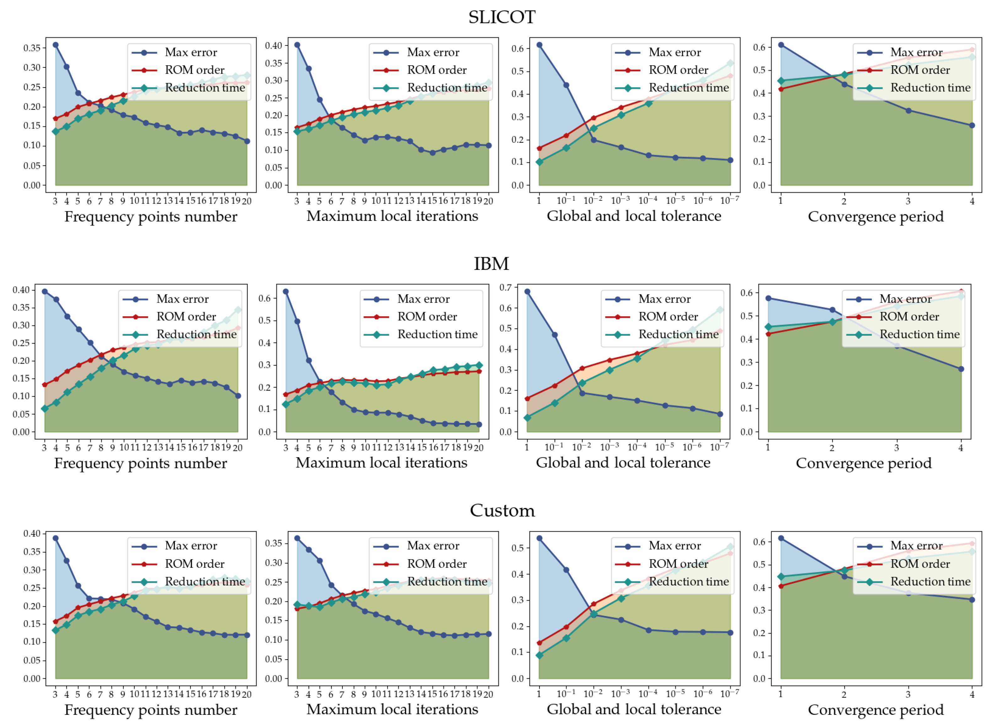
To evaluate the performance of the proposed MPMM method, we compared it against A3PSA [15]. All methods were evaluated using a comprehensive set of benchmarks, including SLICOT models [25], IBM power grids [26], and a variety of custom-designed circuits implemented using GlobalFoundries 22 nm FDSOI technology. The custom benchmarks include a phase-locked loop (PLL), an analog mixer, a time-interleaved digital-to-analog converter (TI_DAC), three low-noise-amplifiers (LNAs), an injection-locked frequency multiplier (ILFM), and a frequency divider (FDIV). Corresponding RLCk models for these designs were generated using ANSYS RaptorH™ [2].

Table 1. Detailed characteristics of the examined RLC and RLCk models.

Model	Order	# Ports	# Mutual Ind.	$\left|\right|{\mathit{G}}_{\mathit{C}}{\left|\right|}_{\mathit{F}}$	$\mathit{cond}\left({\mathit{G}}_{\mathit{C}}\right)$
MNA_1	578	9	0	$2.55\times {10}^{34}$	$4.20\times {10}^{30}$
MNA_2	9223	18	832,068	$1.20\times {10}^{33}$	$4.06\times {10}^{30}$
MNA_3	4863	22	1,336,054	$1.51\times {10}^{34}$	$7.70\times {10}^{31}$
MNA_4	980	4	82,026	$2.76\times {10}^{37}$	$8.91\times {10}^{45}$
ibmpg1t	54,265	20	0	$1.68\times {10}^{11}$	$1.88\times {10}^{18}$
ibmpg2t	164,897	20	0	$6.19\times {10}^{11}$	$1.01\times {10}^{20}$
ibmpg3t	1,043,444	20	0	$3.08\times {10}^{15}$	$1.19\times {10}^{25}$
ibmpg4t	1,214,288	20	0	$4.59\times {10}^{12}$	$2.03\times {10}^{22}$
PLL @ 28 GHz	1474	4	251,680	$7.03\times {10}^{21}$	$4.41\times {10}^{16}$
Mixer @ 28 GHz	1498	10	79,794	$4.13\times {10}^{23}$	$1.81\times {10}^{18}$
TI_DAC @ 28 GHz	3869	160	365,494	$4.16\times {10}^{22}$	$9.62\times {10}^{15}$
LNA @ 56 GHz	4274	6	1,988,882	$1.73\times {10}^{24}$	$1.37\times {10}^{19}$
LNA @ 28 GHz	6956	6	5,360,490	$1.55\times {10}^{23}$	$3.15\times {10}^{18}$
ILFM @ 14 GHz	15,665	11	18,394,794	$4.68\times {10}^{27}$	$9.02\times {10}^{22}$
LNA @ 2.4 GHz	25,602	6	72,959,220	$6.23\times {10}^{23}$	$5.14\times {10}^{19}$
FDIV @ 28 GHz	59,386	10	106,236,284	$2.89\times {10}^{27}$	$1.14\times {10}^{46}$

summarizes the characteristics of all evaluated models. For each benchmark, we report the Frobenius norm $\left|\right|{\mathbf{G}}_C{\left|\right|}_F$ and the condition number $cond\left({\mathbf{G}}_C\right)$ of the system matrix ${\mathbf{G}}_C$.

As indicated in Table 1, the majority of the benchmarks feature a significant number of mutual inductances, and their system matrices are often ill-conditioned, which poses challenges to MOR. Figure 2 shows typical sparsity patterns of the matrices $\mathbf{G}$ and $\mathbf{C}$ for each benchmark category. In RLCk models, the $\mathbf{G}$ matrix and the capacitance sub-matrix ${\mathbf{C}}_n$ are sparse, while the mutual inductance sub-matrix $\mathbf{M}$ is dense due to the high density of electromagnetic coupling.

The MPMM method was initially configured with the following parameters:

• Tolerance thresholds ($target\_error$, $global\_tol$, $local\_tol$) set to ${10}^{-2}$;
• Number of candidate frequency points and maximum local iterations ($freq\_points\_num$, $max\_local\_iters$) set to 7;
• Convergence period ($convergence\_period$) set to 2 iterations.

All algorithms were implemented in C++ using the Eigen library [27] and the experiments were performed on a Linux workstation equipped with a 2.80 GHz 16-thread Intel^® Xeon Silver 4309Y CPU and 64 GB of memory.

5.2. MPMM Parameter Tuning

To determine appropriate parameter values for the MPMM method, we conducted an initial analysis by varying one parameter at a time while keeping the rest fixed according to the above configuration. For each parameter, we evaluated the resulting impact on three key metrics: maximum error, ROM order, and reduction time. All metric values were normalized and then averaged across benchmarks of the same category (SLICOT, IBM, and Custom), providing comparative insight into how each parameter affects performance. The aggregated results are presented in Figure 3.

As demonstrated, increasing the number of frequency points or the maximum local iterations generally improves the ROM accuracy, but at the cost of slightly higher ROM order and runtime. Setting the expansion points to seven and the local iterations to nine was found to provide a good balance between accuracy and efficiency, avoiding unnecessary subspace growth while maintaining precision across all benchmarks. For both global and local convergence tolerances, a value of ${10}^{-2}$ yielded consistently reliable results. Further reducing the tolerance (e.g., to ${10}^{-3}$) did not lead to meaningful accuracy improvements, but increased computational cost and ROM order. Regarding the convergence period, a value of three strikes an effective balance, minimizing unnecessary convergence checks and ensuring timely termination. Based on this analysis, the selected parameters were used for the subsequent evaluation.

5.3. Performance and Accuracy Evaluation

Following the parameter selection, we conducted a comprehensive evaluation to assess the accuracy, ROM order, and runtime performance of MPMM. The results are presented in

Table 2. Comparison of MPMM and A3PSA in terms of ROM accuracy, ROM order, reduction time, and memory requirements across the examined RLC and RLCk models.

Model	ROM Order for Same Error		Max Error for Same Order		Reduction Time for Same Order		Memory for Same Order
	MPMM	A3PSA	MPMM	A3PSA	MPMM	A3PSA	MPMM	A3PSA
MNA_1	207	243	$2.46\times {10}^{-5}$	$5.14\times {10}^{-5}$	0.3 s	0.4 s	41 MB	45 MB
MNA_2	234	324	$1.11\times {10}^{-6}$	$1.24\times {10}^{-2}$	4 s	5 s	363 MB	364 MB
MNA_3	352	594	$2.27\times {10}^{-11}$	$8.05\times {10}^{-7}$	3 s	8 s	306 MB	285 MB
MNA_4	60	180	$2.84\times {10}^{-8}$	$2.29\times {10}^{-4}$	0.17 s	0.25 s	46 MB	47 MB
ibmpg1t	440	540	$1.91\times {10}^{-2}$	$2.06\times {10}^{-2}$	30 s	45 s	921 MB	1.34 GB
ibmpg2t	360	300	$9.37\times {10}^{-4}$	$1.85\times {10}^{-3}$	38 s	2 min	2.5 GB	2.3 GB
ibmpg3t	440	540	$1.53\times {10}^{-3}$	$2.74\times {10}^{-2}$	12 min	16 min	16.1 GB	24.6 GB
ibmpg4t	360	540	$2.05\times {10}^{-5}$	$6.48\times {10}^{-4}$	6 min	13 min	15.9 GB	15.5 GB
PLL @ 28 GHz	36	88	$6.28\times {10}^{-9}$	$9.52\times {10}^{-3}$	0.3 s	1 s	73 MB	67 MB
Mixer @ 28 GHz	60	180	$1.23\times {10}^{-9}$	$1.51\times {10}^{-5}$	0.2 s	0.3 s	49 MB	56 MB
TI_DAC @ 28 GHz	640	1440	$4.21\times {10}^{-6}$	$2.01\times {10}^{-4}$	5 s	12 s	255 MB	635 MB
LNA @ 56 GHz	108	138	$1.51\times {10}^{-4}$	$1.12\times {10}^{-3}$	2 s	8 s	295 MB	271 MB
LNA @ 28 GHz	108	126	$9.58\times {10}^{-4}$	$5.47\times {10}^{-3}$	4 s	12 s	675 MB	686 MB
ILFM @ 14 GHz	231	3762	$1.23\times {10}^{-3}$	$1.42\times {10}^{-2}$	51 s	1 min	1.8 GB	2.1 GB
LNA @ 2.4 GHz	96	270	$2.67\times {10}^{-3}$	$4.12\times {10}^{-2}$	2 min	6 min	7.2 GB	7.9 GB
FDIV @ 28 GHz	150	180	$3.77\times {10}^{-3}$	$4.29\times {10}^{-3}$	6 min	18 min	9.4 GB	10.5 GB

, where the maximum relative error is computed as $\left|\right|\mathbf{H}\left(s\right)-\tilde{\mathbf{H}}{\left(s\right)\left|\right|}_{\infty }/{\left|\right|\mathbf{H}\left(s\right)\left|\right|}_{\infty }$, evaluated over a set of frequency points. For the SLICOT benchmarks, the evaluation was performed over the frequency range [$f_{min},f_{max}$] = [${10}^{-6}$,${10}^6$], while for the IBM power grid circuits, the range was set to [$f_{min},f_{max}$] = [${10}^8$,${10}^{11}$]. In the case of custom RLCk designs, we used a base frequency of 100 MHz ($f_{min}$ = ${10}^8$), and the upper bound was set to twice the resonance frequency of each circuit. For instance, the PLL operating at 28 GHz was evaluated up to 56 GHz ($f_{max}$ = $56\times {10}^9$). Initially, we obtained the MPMM ROMs using the discussed parameters and calculated the corresponding errors. Then, to ensure a fair comparison, we evaluated A3PSA under two scenarios. First, A3PSA ROMs were generated until the resulting errors matched those of the MPMM ROMs, and the corresponding ROM orders were recorded (i.e., ROM order for same error). Second, A3PSA was run to produce ROMs of the same order as the MPMM ROMs, and the resulting maximum errors were measured (i.e., max error for same order). Runtime measurements were also conducted under equal ROM size to reflect algorithmic performance.

As shown in Table 2, the proposed MPMM method consistently produces either more accurate ROMs for the same order or smaller ROMs for the same error compared to A3PSA. This trend holds across all benchmark categories. For example, in the PLL @ 28 GHz benchmark, MPMM achieves significantly lower error ($6.28\times {10}^{-9}$ vs. $9.52\times {10}^{-3}$) for the same ROM order. As illustrated in Figure 4, the MPMM ROM closely follows the original transfer function, whereas A3PSA slightly deviates, particularly near the mid and high frequencies. Similarly, in the MNA_2 case, although both methods reduce the model to a few hundred states, A3PSA exhibits a noticeable accuracy drop, with a maximum error of $1.24\times {10}^{-2}$ compared to only $1.11\times {10}^{-6}$ for MPMM.

The advantage of MPMM becomes more pronounced in large and complex circuits. For instance, in the TI_DAC @ 28 GHz benchmark, MPMM achieves the same accuracy as A3PSA with a ROM that is 2.25× smaller (640 vs. 1440), while also reducing memory usage by more than half. In addition, in the ibmpg3t case, MPMM delivers a lower maximum error ($1.53\times {10}^{-3}$ vs. $2.74\times {10}^{-2}$) with a more compact ROM and efficient memory consumption. As depicted in Figure 5, although A3PSA matches the original transfer function at ports (12,7), it exhibits noticeable deviations at ports (2,9), which deteriorate at ports (4,7). In contrast, MPMM consistently preserves accuracy across all examined ports.

To further validate the accuracy of the proposed approach, Figure 6 shows representative ROM transfer functions for each benchmark category, demonstrating that MPMM consistently results in more accurate ROMs across all cases. To highlight the superiority of MPMM over A3PSA, Figure 7 presents the root mean square (RMS) error between the original and reduced transfer function matrices for different benchmarks. As can be seen, MPMM achieves a lower RMS error for nearly all port combinations, with A3PSA exhibiting visible regions of higher error. This indicates that the proposed approach maintains high ROM accuracy for all input–output ports in the examined frequency range.

Beyond its accuracy advantages, MPMM is highly effective at producing compact models. Across all evaluated benchmarks, MPMM achieves reductions ranging from 64.18% to 99.97%, with large-scale models (>20 K nodes) typically reduced by more than 99.18%. Furthermore, it yields ROMs that are 2.6× on average and up to 16.3× more compact than A3PSA ROMs for the same level of accuracy. ROM compactness results from the adaptive control over the number of moments matched per frequency, achieved through local convergence checks in MPMM. Unlike A3PSA, which uses a fixed number of moments per expansion point [15], MPMM dynamically adjusts the subspace size, avoiding unnecessary computation while maintaining accuracy.

In terms of reduction performance, MPMM achieves up to 4× speedup over A3PSA, with an average of 2.3× faster execution. This improvement is particularly evident in complex designs such as FDIV @ 28 GHz and ibmpg4t, where A3PSA’s fixed iteration scheme leads to longer runtimes. MPMM avoids such inefficiencies through its less frequent convergence checks and adaptive termination strategy. Even greater speedup could be achieved by configuring MPMM to match the accuracy of A3PSA.

Regarding memory requirements, although the memory usage of MPMM is comparable to that of A3PSA on smaller benchmarks, it performs notably better in large-scale designs. For example, in ibmpg1t and ibmpg3t, MPMM reduces memory consumption by over 400 MB and 8.5 GB, respectively, while achieving superior or similar accuracy. Moreover, for the TI_DAC @ 28 GHz benchmark, MPMM requires 2.5× less memory than A3PSA. Combined with its faster runtime, improved accuracy, and more compact ROMs, MPMM achieves an optimal balance between performance and precision. These advantages make MPMM especially suitable for reducing real-world designs encountered in industrial applications.

We also tested our method against several established techniques, including tangential IRKA [12], ISRK [5], RKSM [6], and LR-ADI [28], using implementations from open-source frameworks such as M-M.E.S.S. [29], sssMOR [30], and MATLAB’s reducespec toolbox [31]. However, the results from these comparisons are not reported in this article due to several limitations observed during evaluation. Specifically, these methods either required high ROM orders to reach acceptable accuracy, failed to converge reliably on several benchmarks, or incurred excessive computational demands.

6. Conclusions

This article presents a frequency-aware MM MOR method based on the RKS, tailored for the efficient reduction in large-scale RLCk models. The proposed MPMM technique employs adaptive expansion point selection, local and global convergence criteria, and several efficient implementation strategies to efficiently handle large-scale models. Unlike existing methods, MPMM relies exclusively on the ROM transfer function to drive the subspace construction and adaptively determines the required number of moments per expansion point. Experimental results indicate that MPMM consistently outperforms A3PSA, producing ROMs that are on average 2.6× and up to 16.3× smaller, achieving up to 99.97% reduction for large-scale benchmarks. Additionally, MPMM achieves an average of 2.3× and up to 4× runtime speedup compared to A3PSA. These improvements demonstrate that the proposed method is well suited for practical deployment in industrial tools such as ANSYS RaptorH™ [2] for passive RLCk model reduction.

References

1. Liu, M. 1.1 Unleashing the Future of Innovation. In Proceedings of the IEEE International Solid-State Circuits Conference (ISSCC), San Francisco, CA, USA, 13–17 February 2021; pp. 9–16. [Google Scholar]
2. Ansys—RaptorH™. Available online: www.ansys.com/products/semiconductors/ansys-raptorh (accessed on 23 June 2025).
3. Phillips, J.; Daniel, L.; Silveira, L.M. Guaranteed Passive Balancing Transformations for Model Order Reduction. In Proceedings of the 39th Annual Design Automation Conference (DAC), New Orleans, LA, USA, 10–14 June 2002; pp. 52–57. [Google Scholar]
4. Gugercin, S.; Antoulas, A.C. A Survey of Model Reduction by Balanced Truncation and Some New Results. Int. J. Control 2004, 77, 748–766. [Google Scholar] [CrossRef]
5. Gugercin, S. An Iterative SVD-Krylov Based Method for Model Reduction of Large-Scale Dynamical Systems. Linear Algebra Appl. 2008, 428, 1964–1986. [Google Scholar] [CrossRef]
6. Druskin, V.; Simoncini, V. Adaptive Rational Krylov Subspaces for Large-Scale Dynamical Systems. Syst. Control Lett. 2011, 60, 546–560. [Google Scholar] [CrossRef]
7. Floros, G.; Evmorfopoulos, N.; Stamoulis, G. Frequency-Limited Reduction of Regular and Singular Circuit Models via Extended Krylov Subspace Method. IEEE Trans. Very Large Scale Integr. (VLSI) Syst. 2020, 28, 1610–1620. [Google Scholar] [CrossRef]
8. Giamouzis, C.; Garyfallou, D.; Stamoulis, G.; Evmorfopoulos, N. Low-Rank Balanced Truncation of RLCk Models via Frequency-Aware Rational Krylov-Based Projection. In Proceedings of the 20th International Conference on Synthesis, Modeling, Analysis and Simulation Methods and Applications to Circuit Design (SMACD), Coimbra, Portugal, 1–4 July 2024; pp. 1–4. [Google Scholar]
9. Grivet-Talocia, S.; Ubolli, A. A Comparative Study of Passivity Enforcement Schemes for Linear Lumped Macromodels. IEEE Trans. Adv. Packag. 2008, 31, 673–683. [Google Scholar] [CrossRef]
10. Odabasioglu, A.; Celik, M.; Pileggi, L. PRIMA: Passive Reduced-order Interconnect Macromodeling Algorithm. IEEE Trans. Comput.-Aided Des. Integr. Circuits Syst. 1998, 17, 645–654. [Google Scholar] [CrossRef]
11. Freund, R.W. SPRIM: Structure-Preserving Reduced-Order Interconnect Macromodeling. In Proceedings of the IEEE/ACM International Conference on Computer-Aided Design (ICCAD), San Jose, CA, USA, 7–11 November 2004; pp. 80–87. [Google Scholar]
12. Gugercin, S.; Antoulas, A.C.; Beattie, C. H2 Model Reduction for Large-Scale Linear Dynamical Systems. SIAM J. Matrix Anal. Appl. 2008, 30, 609–638. [Google Scholar] [CrossRef]
13. Panzer, H.K. Model Order Reduction by Krylov Subspace Methods with Global Error Bounds and Automatic Choice of Parameters. Ph.D. Thesis, Technische Universität München, Munich, Germany, 2014. [Google Scholar]
14. Feng, L.; Korvink, J.G.; Benner, P. A Fully Adaptive Scheme for Model Order Reduction Based on Moment Matching. IEEE Trans. Compon. Packag. Manuf. Technol. 2015, 5, 1872–1884. [Google Scholar] [CrossRef]
15. Nguyen, T.S.; Le Duc, T.; Tran, T.S.; Guichon, J.M.; Chadebec, O.; Meunier, G. Adaptive Multipoint Model Order Reduction Scheme for Large-Scale Inductive PEEC Circuits. IEEE Trans. Electromagn. Compat. 2017, 59, 1143–1151. [Google Scholar] [CrossRef]
16. Chatzigeorgiou, C.; Garyfallou, D.; Floros, G.; Evmorfopoulos, N.; Stamoulis, G. Exploiting Extended Krylov Subspace for the Reduction of Regular and Singular Circuit Models. In Proceedings of the 26th Asia and South Pacific Design Automation Conference (ASPDAC), Tokyo, Japan, 18–21 January 2021; pp. 773–778. [Google Scholar]
17. Hamadi, M.A.; Jbilou, K.; Ratnani, A. A Model Reduction Method in Large-Scale Dynamical Systems Using an Extended-Rational Block Arnoldi Method. J. Appl. Math. Comput. 2022, 68, 271–293. [Google Scholar] [CrossRef]
18. Nakatsukasa, Y.; Sète, O.; Trefethen, L.N. The AAA Algorithm for Rational Approximation. SIAM J. Sci. Comput. 2018, 40, A1494–A1522. [Google Scholar] [CrossRef]
19. Bradde, T.; Grivet-Talocia, S.; Aumann, Q.; Gosea, I.V. A Modified AAA Algorithm for Learning Stable Reduced-Order Models from Data. J. Sci. Comput. 2025, 103, 14. [Google Scholar] [CrossRef]
20. Lemus, A.; Ege Engin, A. AGORA: Adaptive Generation of Orthogonal Rational Approximations for Frequency-Response Data. Int. J. Circuit Theory Appl. 2025. [Google Scholar] [CrossRef]
21. Ho, C.W.; Ruehli, A.E.; Brennan, P.A. The Modified Nodal Approach to Network Analysis. IEEE Trans. Circuits Syst. 1975, 22, 504–509. [Google Scholar]
22. Gröchenig, K. Foundations of Time-Frequency Analysis; Birkhäuser: Boston, MA, USA, 2001. [Google Scholar]
23. Golub, G.H.; Van Loan, C.F. Matrix Computations; Johns Hopkins University Press: Baltimore, MD, USA, 1983. [Google Scholar]
24. Grimme, E.J. Krylov Projection Methods for Model Reduction. Ph.D. Thesis, University of Illinois at Urbana-Champaign, Urbana, IL, USA, 1997. [Google Scholar]
25. Chahlaoui, Y.; Van Dooren, P. A Collection of Benchmark Examples for Model Reduction of Linear Time Invariant Dynamical Systems; Technical Report, SLICOT Working Note 2002-2; 2002. Available online: https://eprints.maths.manchester.ac.uk/1040/ (accessed on 23 June 2025).
26. Nassif, S.R. Power Grid Analysis Benchmarks. In Proceedings of the 13th Asia and South Pacific Design Automation Conference (ASPDAC), Seoul, Republic of Korea, 21–24 January 2008; pp. 376–381. [Google Scholar]
27. Guennebaud, G.; Jacob, B.; Niesen, J.; Heibel, H.; Gautier, M.; Olivier, S.; Steiner, B.; Riddile, K.; Capricelli, T.; Holoborodko, P.; et al. Eigen v3. Available online: http://eigen.tuxfamily.org (accessed on 23 June 2025).
28. Benner, P.; Breiten, T. Low Rank Methods for a Class of Generalized Lyapunov Equations and Related Issues. Numer. Math. 2013, 124, 441–470. [Google Scholar] [CrossRef]
29. M-M.E.S.S.-3.0—The Matrix Equations Sparse Solvers Library. Available online: https://www.mpi-magdeburg.mpg.de/projects/mess (accessed on 23 June 2025).
30. MORLab—sssMOR Toolbox. Available online: https://www.mathworks.com/matlabcentral/fileexchange/59169-sssmor-toolbox (accessed on 23 June 2025).
31. MathWorks—Reducespec. Available online: https://www.mathworks.com/help/matlab/ref/reducespec.html (accessed on 23 June 2025).
Figure 1. Final rational Krylov subspace generated by the proposed MPMM approach.
Technologies 13 00274 g001
Figure 2. Sparsity patterns of matrices G and C of MNA_2, ILFM @ 14 GHz, and ibmpg2t.
Technologies 13 00274 g002
Figure 3. Normalized average ROM order, maximum error, and reduction time across each benchmark category (SLICOT, IBM, Custom) for varying MPMM parameter values.
Technologies 13 00274 g003
Figure 4. Comparison of the original and ROM transfer functions of PLL @ 28 GHz across ports (3,3) for identical MPMM and A3PSA ROM order. The plots demonstrate the frequency responses at (a) the examined frequency range, (b) the resonance frequency, and (c) the high-frequency region.
Technologies 13 00274 g004
Figure 5. Comparison of the original and ROM transfer functions of ibmpg3t at ports (a) (12,7), (b) (2,9), and (c) (4,7) for identical MPMM and A3PSA ROM order.
Technologies 13 00274 g005
Figure 6. Comparison of the original and ROM transfer functions of (a) MNA_2 at ports (8,9), (b) ibmpg1t at ports (14,15), and (c) TI_DAC @ 28 GHz at ports (2,5) for identical MPMM and A3PSA ROM order.
Technologies 13 00274 g006
Figure 7. RMS errors of MPMM and A3PSA ROM transfer functions across all input–output port combinations for MNA_2, ibmpg2t, and Mixer @ 28 GHz.
Technologies 13 00274 g007