
Ultra-Wideband Antenna Design for 5G NR Using the Bezier Search Differential Evolution Algorithm
 ,
,  ,
,  ,
,  , ,
, ,  , and
, and 
Abstract
1. Introduction
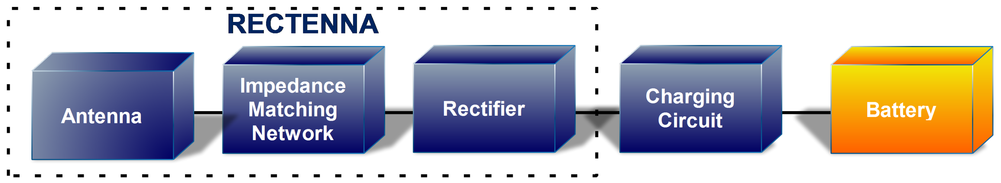
- We design a novel ultra-wide band antenna for RF energy harvesting applications with more than a 2 GHz bandwidth.
- We introduce a recent optimization algorithm (BeSD) for antenna design. To the best of our knowledge, this is the first time BeSD has been applied to an optimization problem in electromagnetics.
2. Materials and Methods
2.1. Optimization Process
2.2. Matlab—CST API
2.3. Bezier Search Differential Evolution Algorithm Desctiption
- Its unique (Benzier polyonimials) mutation algorithm is multi-component, including a weighted-elitist component that strengthens exploitation. It differs from the mutation operators of conventional algorithms, providing an enhanced exploration aspect to BeSD.
- In contrast to most conventional algorithms, its crossover process has no control parameters and is randomized, favoring both exploration and exploitation.
- BeSD’s characteristic structure showcases simplicity and efficiency, due to its limited computational complexity, which leads to accurate optimal solutions with a relatively quick convergence, compared to conventional algorithms.
- Moreover, BeSD can be applied to parallel computing scenarios, as its patterns evolve separately, leading to a non-recursive algorithm.
| Algorithm 1 Pseudo-code for the Bezier Search Differential Evolution Algorithm. |
|
2.4. Performance Evaluation
- Population: 100.
- Iterations: 1000.
- Problem Variables: 30.
- Variable Boundaries: .
- Independent Trials: 100.
3. Optimization Results and Discussion
- Independent Trials: 5.
- Size Control Value of Pre-Pattern Matrix, L: 2.5, to assure balance between exploration and exploitation mechanisms.
- Number of Iterations: 100.
- Size of Pattern Matrix, N (Size of Population): 40.
- Problem Dimensions, D (Variables): 3.
- Variable Boundaries:.
- –
- Structure Scaling Factor: .
- –
- Stub Width: (mm).
- –
- Stub Length: (mm).
4. Conclusions
Author Contributions
Funding
Institutional Review Board Statement
Informed Consent Statement
Data Availability Statement
Conflicts of Interest
Appendix A. Benchmark Functions
- 1.
- Rotated Hyper-ellipsoid function:where is an n-dimensional vector.Global solution: .
- 2.
- Rastrigin function:where is an n-dimensional vector and .Global solution: .
- 3.
- Ackley function:where is an n-dimensional vector, and .Global minimum: .
- 4.
- Sphere function:where is an n-dimensional vector.Global solution: .
- 5.
- Powell function:where is an n-dimensional vector, and n is divisible by 4.Global solution: .
- 6.
- Three-Hump Camel function:where is a 2-dimensional vector ().Global solution: .
- 7.
- Beale function:where is a 2-dimensional vector ().Global solution: .
- 8.
- Sum of Squares function:where is an n-dimensional vector.Global solution: .
- 9.
- Bohachevsky No. 3 function:where is a 2-dimensional vector ().Global solution: .
- 10.
- Sum of Different Powers function:where is an n-dimensional vector and p is a positive integer.Global solution: .
References
- Korompilis, G.; Siakavara, K. Synthesis of Ultra-Wideband Rectenna for RF Energy Harvesting From Wireless Communications Networks. In Proceedings of the 2023 12th International Conference on Modern Circuits and Systems Technologies (MOCAST), Athens, Greece, 28–30 June 2023; pp. 1–5. [Google Scholar] [CrossRef]
- Korompilis, G.; Boursianis, A.; Sarigiannidis, P.; Zaharis, Z.; Goudos, S.; Siakavara, K. Ultra-Wideband Antenna Design for RF Energy Harvesting Applications Using the Bald Eagle Search Algorithm. In Proceedings of the 2024 13th International Conference on Modern Circuits and Systems Technologies (MOCAST), Sofia, Bulgaria, 26–28 June 2024. [Google Scholar] [CrossRef]
- Civicioglu, P.; Besdok, E. Bezier Search Differential Evolution Algorithm for numerical function optimization: A comparative study with CRMLSP, MVO, WA, SHADE and LSHADE. Expert Syst. Appl. 2021, 165, 113875. [Google Scholar] [CrossRef]
- Chandravanshi, S.; Sarma, S.S.; Akhtar, M.J. Design of triple band differential rectenna for RF energy harvesting. IEEE Trans. Antennas Propag. 2018, 66, 2716–2726. [Google Scholar]
- Shi, Y.; Jing, J.; Fan, Y.; Yang, L.; Li, Y.; Wang, M. A novel compact broadband rectenna for ambient RF energy harvesting. AEU Int. J. Electron. Commun. 2018, 95, 264–270. [Google Scholar]
- Song, C.; Huang, Y.; Zhou, J.; Zhang, J.; Yuan, S.; Carter, P. A high-efficiency broadband rectenna for ambient wireless energy harvesting. IEEE Trans. Antennas Propag. 2015, 63, 3486–3495. [Google Scholar] [CrossRef]
- Sun, H.; Guo, Y.X.; He, M.; Zhong, Z. A dual-band rectenna using broadband Yagi antenna array for ambient RF power harvesting. IEEE Antennas Wirel. Propag. Lett. 2013, 12, 918–921. [Google Scholar]
- Shen, S.; Zhang, Y.; Chiu, C.Y.; Murch, R. A triple-band high-gain multibeam ambient RF energy harvesting system utilizing hybrid combining. IEEE Trans. Ind. Electron. 2020, 67, 9215–9226. [Google Scholar]
- Shi, Y.; Fan, Y.; Li, Y.; Yang, L.; Wang, M. An efficient broadband slotted rectenna for wireless power transfer at LTE band. IEEE Trans. Antennas Propag. 2019, 67, 814–822. [Google Scholar]
- Alsattar, H.; Zaidan, A.; Zaidan, B. Novel meta-heuristic bald eagle search optimisation algorithm. Artif. Intell. Rev. 2020, 53, 2237–2264. [Google Scholar] [CrossRef]
- Johnson, J.; Rahmat-Samii, V. Genetic algorithms in engineering electromagnetics. IEEE Antennas Propag. Mag. 1997, 39, 7–21. [Google Scholar] [CrossRef]
- Rocca, P.; Oliveri, G.; Massa, A. Differential Evolution as Applied to Electromagnetics. IEEE Antennas Propag. Mag. 2011, 53, 38–49. [Google Scholar] [CrossRef]
- Robinson, J.; Rahmat-Samii, Y. Particle swarm optimization in electromagnetics. IEEE Trans. Antennas Propag. 2004, 52, 397–407. [Google Scholar] [CrossRef]
- Li, X.; Luk, K.M. The Grey Wolf Optimizer and Its Applications in Electromagnetics. IEEE Trans. Antennas Propag. 2020, 68, 2186–2197. [Google Scholar] [CrossRef]
- Gregory, M.D.; Martin, S.V.; Werner, D.H. Improved electromagnetics optimization: The covariance matrix adaptation evolutionary strategy. IEEE Antennas Propag. Mag. 2015, 57, 48–59. [Google Scholar] [CrossRef]
- Mussetta, M.; Grimaccia, F.; Zich, R.E. Comparison of different optimization techniques in the design of electromagnetic devices. In Proceedings of the 2012 IEEE Congress on Evolutionary Computation, Brisbane, QLD, Australia, 10–15 June 2012; pp. 1–6. [Google Scholar] [CrossRef]
- Holland, J. Genetic Algorithms. Sci. Am. 1992, 267, 66–73. [Google Scholar]
- Back, T. Evolutionary Algorithms in Theory and Practice: Evolution Strategies, Evolutionary Programming, Genetic Algorithms; Oxford University Press: Oxford, UK, 1996. [Google Scholar]
- Kennedy, J.; Eberhart, R. Particle swarm optimization. In Proceedings of the ICNN’95—International Conference on Neural Networks, Perth, WA, Australia, 27 November–1 December 1995; Volume 4, pp. 1942–1948. [Google Scholar] [CrossRef]
- Zhang, Y.; Wang, S.; Ji, G. A comprehensive survey on particle swarm optimization algorithm and its applications. Math. Probl. Eng. 2015, 2015, 931256. [Google Scholar] [CrossRef]
- Mirjalili, S.; Mirjalili, S.M.; Lewis, A. Grey Wolf Optimizer. Adv. Eng. Softw. 2014, 69, 46–61. [Google Scholar] [CrossRef]
- Makhadmeh, S.N.; Al-Betar, M.A.; Doush, I.A.; Awadallah, M.A.; Kassaymeh, S.; Mirjalili, S.; Zitar, R.A. Recent advances in grey wolf optimizer, its versions and applications: Review. IEEE Access 2024, 12, 22991–23028. [Google Scholar]
- Storn, R.; Price, K. Differential Evolution—A Simple and Efficient Heuristic for Global Optimization over Continuous Spaces. J. Glob. Optim. 1997, 11, 341–359. [Google Scholar] [CrossRef]
- Hansen, N.; Müller, S.; Koumoutsakos, P. Reducing the Time Complexity of the Derandomized Evolution Strategy with Covariance Matrix Adaptation (CMA-ES). Evol. Comput. 2003, 11, 1–18. [Google Scholar] [CrossRef]
- Simon, D. Biogeography-Based Optimization. IEEE Trans. Evol. Comput. 2008, 12, 702–713. [Google Scholar]
- Ma, H.; Simon, D.; Siarry, P.; Yang, Z.; Fei, M. Biogeography-based Optimization: A 10-Year Review. IEEE Trans. Emerg. Top. Comput. Intell. 2017, 1, 391–407. [Google Scholar]
- Akgüngör, A.P.; Korkmaz, E. Bezier Search Differential Evolution algorithm basedestimation models of delay parameter k forsignalized intersections. Concurr. Comput. Pract. Exp. 2022, 34, e6931. [Google Scholar] [CrossRef]
- Chen, L.; Zheng, Z.; Liu, H.L.; Xie, S. An evolutionary algorithm based on Covariance Matrix Leaning and Searching Preference for solving CEC 2014 benchmark problems. In Proceedings of the 2014 IEEE Congress on Evolutionary Computation (CEC), Beijing, China, 6–11 July 2014; pp. 2672–2677. [Google Scholar] [CrossRef]
- Erlich, I.; Rueda, J.L.; Wildenhues, S.; Shewarega, F. Solving the IEEE-CEC 2014 expensive optimization test problems by using single-particle MVMO. In Proceedings of the 2014 IEEE Congress on Evolutionary Computation (CEC), Beijing, China, 6–11 July 2014; pp. 1084–1091. [Google Scholar] [CrossRef]
- Ray, T.; Asafuddoula, M. Competition on Real-Parameter Single Objective Expensive Optimization: A Simple Algorithm Without Approximation. Available online: http://www.mdolab.net/Ray/Research-Data/Paper.pdf (accessed on 1 January 2025).
- Tanabe, R.; Fukunaga, A. Success-history based parameter adaptation for Differential Evolution. In Proceedings of the 2013 IEEE Congress on Evolutionary Computation, Cancun, Mexico, 20–23 June 2013; pp. 71–78. [Google Scholar] [CrossRef]
- Tanabe, R.; Fukunaga, A.S. Improving the search performance of SHADE using linear population size reduction. In Proceedings of the 2014 IEEE Congress on Evolutionary Computation (CEC), Beijing, China, 6–11 July 2014; pp. 1658–1665. [Google Scholar] [CrossRef]
- Boursianis, A.; Papadopoulou, M.; Nikolaidis, S.; Sarigiannidis, P.; Psannis, K.; Georgiadis, A.; Tentzeris, M.; Goudos, S. Novel Design Framework for Dual-Band Frequency Selective Surfaces Using Multi-Variant Differential Evolution. Mathematics 2021, 9, 2381. [Google Scholar] [CrossRef]
- Wolpert, D.; Macready, W. No free lunch theorems for optimization. IEEE Trans. Evol. Comput. 1997, 1, 67–82. [Google Scholar] [CrossRef]

| Reference | Design Type | Frequency Bands |
|---|---|---|
| [4] | square, two layer, coupled antenna | 2.1 GHz, 2.4–2.48 GHz, and 3.3–3.8 GHz |
| [5] | slotted fractal patch antenna with partial grounding | 2.15–2.9 GHz |
| [6] | cross-dipole slotted antenna | 1.8–2.5 GHz |
| [7] | 1 × 4 quasi-Yagi-Uda antenna array | 1.8–2.2 GHz |
| [8] | 16-port dual-polarized patch antenna | 1.74–2.57 GHz |
| [9] | compact slotted patch antenna | 2.1–3.5 GHz |
| [1] | wideband patch antenna with slots, stubs, and partial grounding | 1.7–2.7 GHz |
| [2] | wideband patch antenna with stubs and partial grounding, optimized with BES [10] | 1.7–2.7 GHz |
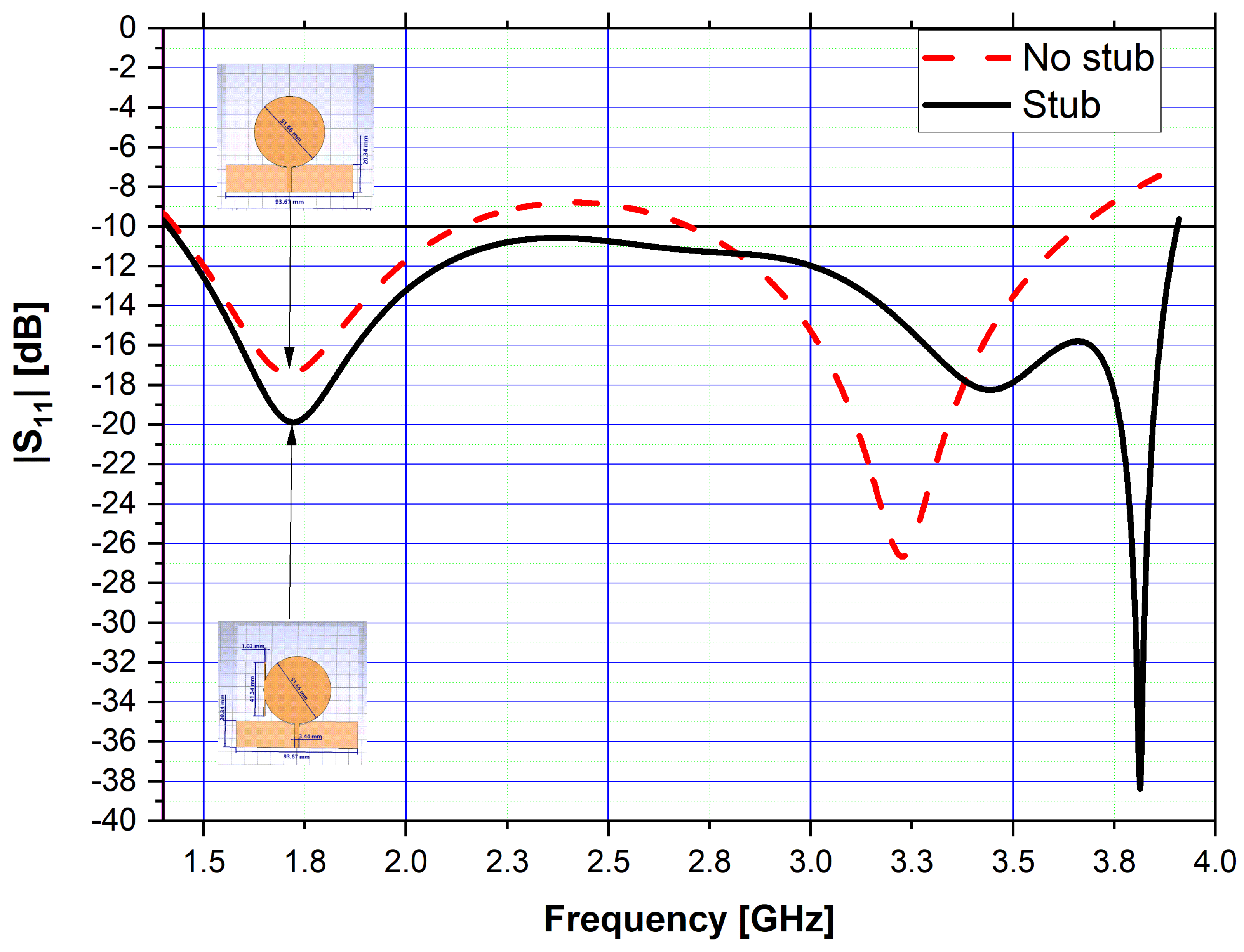
| proposed patch antenna | ultra-wideband patch antenna with a stub and partial grounding, optimized with BeSD [3] | 1.4–3.9 GHz |
| BeSD | GA | BBO | DE | CMA-ES | |
|---|---|---|---|---|---|
| 0.000 × 1000 | 1.170 × 10⁻³³ | 1.606 × 10−02 | 4.216 × 10⁻¹³ | 5.819 × 10⁻²⁵ | |
| 0.000 × 1000 | 13.867 × 1000 | 3.349 × 1000 | 5.980 × 1001 | 1.593 × 1002 | |
| 0.000 × 1000 | 1.563 × 10⁻¹² | 0.491 × 10−01 | 7.846 × 10−09 | 9.731 × 10⁻¹⁰ | |
| 0.000 × 1000 | 9.356 × 10⁻³³ | 2.149 × 10−02 | 7.462 × 10⁻¹⁶ | 9.874 × 10⁻³⁰ | |
| 0.000 × 1000 | 6.950 × 10−02 | 4.350 × 10−02 | 1.429 × 1002 | 9.343 × 1003 | |
| 0.000 × 1000 | 0.000 × 1000 | 5.343 × 10−60 | 2.625 × 10−73 | 3.118 × 10−08 | |
| 5.580 × 10−08 | 0.000 × 1000 | 3.592 × 10⁻¹⁵ | 1.987 × 10⁻²¹ | 8.680 × 10−07 | |
| 0.000 × 1000 | 2.478 × 10⁻³⁴ | 2.027 × 10−02 | 3.771 × 10⁻¹³ | 1.800 × 10⁻²⁶ | |
| 0.000 × 1000 | 0.000 × 1000 | 1.665 × 10⁻¹⁵ | 0.000 × 1000 | 1.296 × 10−06 | |
| 0.000 × 1000 | 4.005 × 10⁻¹⁸ | 1.131 × 10⁻¹⁵ | 1.976 × 10−38 | 4.778 × 10⁻¹² |
| BeSD | GA | BBO | DE | CMA-ES | |
|---|---|---|---|---|---|
| Friedman | |||||
| Normalized Ranking | 1 | 2 | 4 | 3 | 5 |
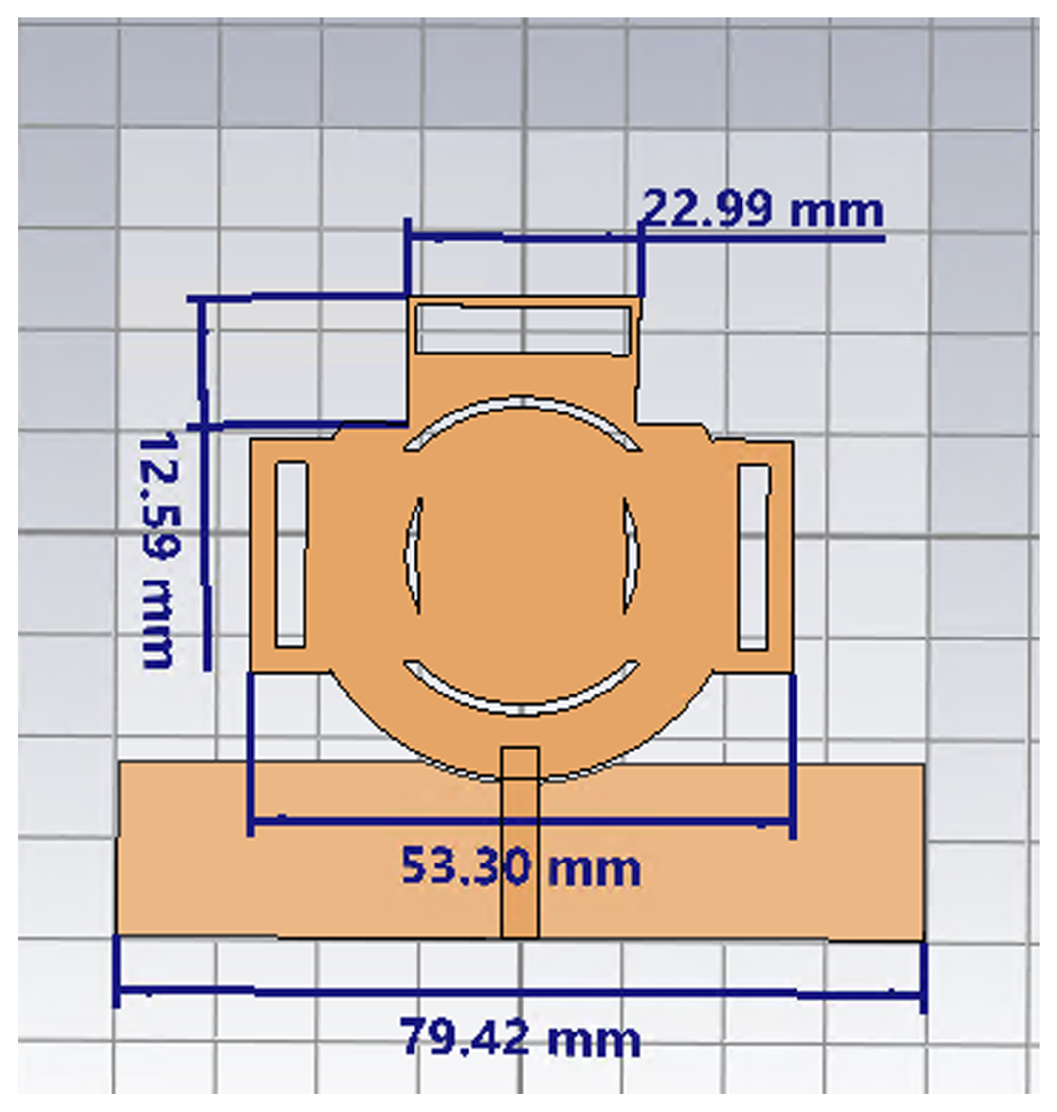
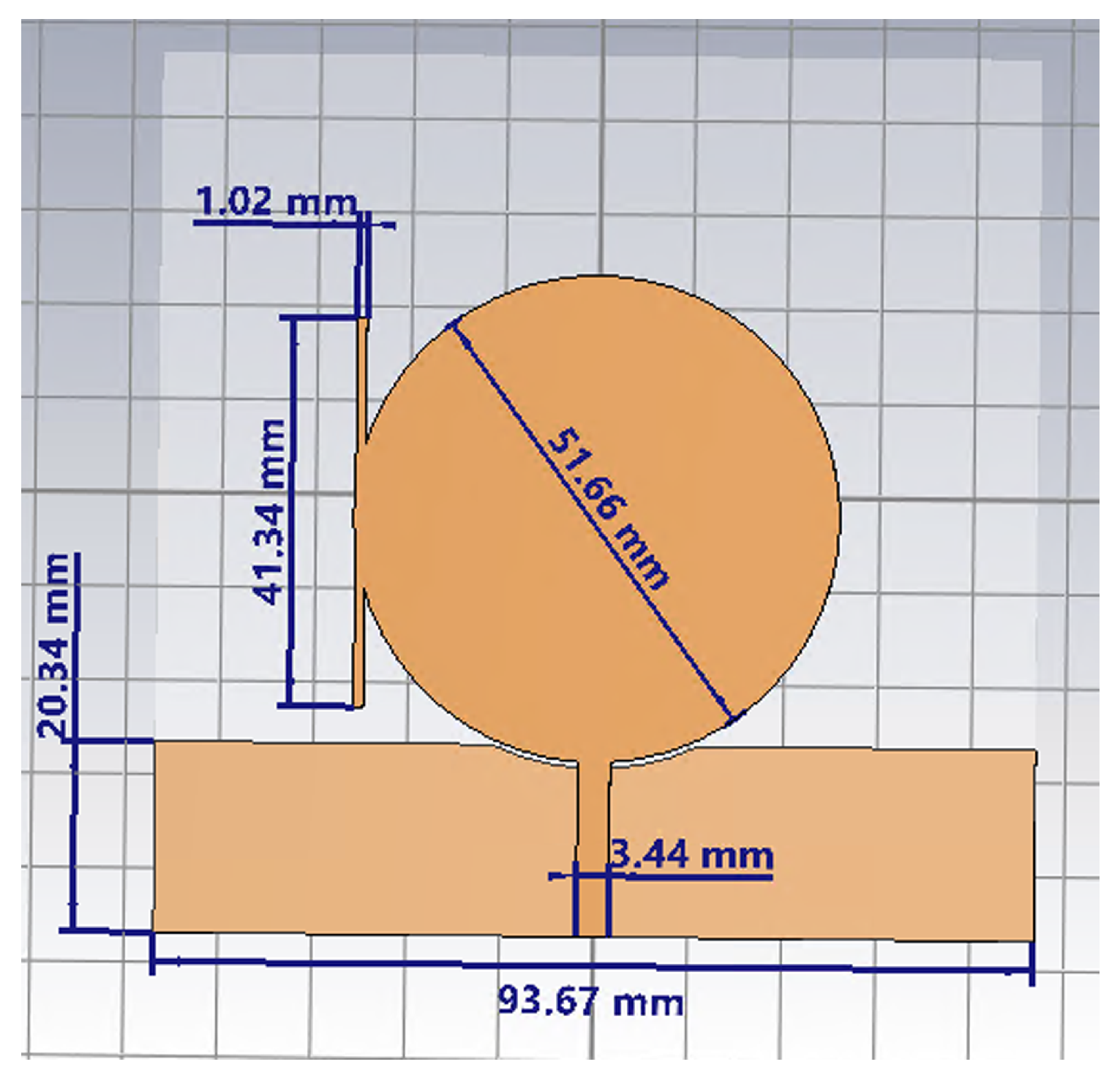
| Parameter | Value (mm) |
|---|---|
| Stub width | 1.02 |
| Stub length | 41.34 |
| Circular patch diameter | 51.66 |
| Substrate side | 93.67 |
| Ground small side | 20.34 |
| Transmission line width | 3.44 |
| Frequency (GHz) | Efficiency |
|---|---|
| 1.8 (GSM) | 95.9% |
| 2.1 (UMTS) | 87.9% |
| 2.4 (Wi-Fi) | 83.7% |
| 2.6 (LTE) | 84.1% |
| 3.5 (5G NR) | 91.8% |
Disclaimer/Publisher’s Note: The statements, opinions and data contained in all publications are solely those of the individual author(s) and contributor(s) and not of MDPI and/or the editor(s). MDPI and/or the editor(s) disclaim responsibility for any injury to people or property resulting from any ideas, methods, instructions or products referred to in the content. |
© 2025 by the authors. Licensee MDPI, Basel, Switzerland. This article is an open access article distributed under the terms and conditions of the Creative Commons Attribution (CC BY) license (https://creativecommons.org/licenses/by/4.0/).
Share and Cite
Korompilis, G.; Boursianis, A.D.; Sarigiannidis, P.; Zaharis, Z.D.; Siakavara, K.; Papadopoulou, M.S.; Matin, M.A.; Goudos, S.K. Ultra-Wideband Antenna Design for 5G NR Using the Bezier Search Differential Evolution Algorithm. Technologies 2025, 13, 133. https://doi.org/10.3390/technologies13040133
Korompilis G, Boursianis AD, Sarigiannidis P, Zaharis ZD, Siakavara K, Papadopoulou MS, Matin MA, Goudos SK. Ultra-Wideband Antenna Design for 5G NR Using the Bezier Search Differential Evolution Algorithm. Technologies. 2025; 13(4):133. https://doi.org/10.3390/technologies13040133
Chicago/Turabian StyleKorompilis, Georgios, Achilles D. Boursianis, Panagiotis Sarigiannidis, Zaharias D. Zaharis, Katherine Siakavara, Maria S. Papadopoulou, Mohammad Abdul Matin, and Sotirios K. Goudos. 2025. "Ultra-Wideband Antenna Design for 5G NR Using the Bezier Search Differential Evolution Algorithm" Technologies 13, no. 4: 133. https://doi.org/10.3390/technologies13040133
APA StyleKorompilis, G., Boursianis, A. D., Sarigiannidis, P., Zaharis, Z. D., Siakavara, K., Papadopoulou, M. S., Matin, M. A., & Goudos, S. K. (2025). Ultra-Wideband Antenna Design for 5G NR Using the Bezier Search Differential Evolution Algorithm. Technologies, 13(4), 133. https://doi.org/10.3390/technologies13040133