Allocation of Single and Multiple Multi-Type Distributed Generators in Radial Distribution Network Using Mountain Gazelle Optimizer

Abstract

The growing demand for clean, reliable and efficient power supply has driven the adoption of renewable energy sources in the package of distributed generation (DG) at the distribution segment of the power system. Despite advancements in DG allocation methodologies, a significant research gap exists regarding the simultaneous evaluation of DG sizing, location and power factor optimization, and their economic implications. This study presents the Mountain Gazelle Optimizer (MGO), a recent optimization approach to address the challenges of sizing, locating, and optimizing the power factor of multi-type DG units in a radial distribution network (RDN). In this work, the MGO is employed to reduce voltage variations, reactive power losses, real power losses, and costs while improving the bus voltage in the RDNs. The methodology involves extensive simulations across multiple scenarios covering one to three DG allocations with varying power factors (unity, fixed, and optimal). Key performance metrics evaluated included real and reactive loss reductions, voltage profile index (VPI), voltage stability index (VSI), and cost reductions due to energy losses compared to base cases. The proposed approach was implemented on the standard 33- and 69-bus networks, and the findings demonstrate that the MGO much outperforms other optimization approaches in the existing literature, realizing considerable decreases in real power losses (up to 98.10%) and reactive power losses (up to 93.38%), alongside notable cost savings. This research showcases the critical importance of optimizing DG power factors, a largely neglected aspect in most prior studies. In conclusion, this work fills a vital gap by integrating power factor optimization into the DG allocation framework, offering a comprehensive approach to enhancing the electricity distribution networks’ dependability, efficacy, and sustainability.

1. Introduction

The distribution stage is essential to the power system as it connects and delivers power from the national grid to the final consumers. Most of the distribution in developing nations is radial, as there is only a one-way power flow from the sub-station to lateral parts of the networks [1]. These radial distribution networks (RDNs) are characterized by non-linear loads, greater resistance to reactance ratio compared to transmission systems, many nodes, untransposed lines, and unbalanced loads [2]. These attributes lead to high power and voltage drop, leading to inefficient and unreliable end-user delivery.

Penetration of distributed generation into the RDN can effectively combat power loss and voltage instability challenges while meeting the ever-increasing population’s electricity demand [3]. Improvement of the system voltage profile and minimization of power loss can be achieved by adequately positioning and sizing DGs integrated into RDNs. Furthermore, including DG can cause the grid reinforcement to be delayed and transmission line capacity to be reduced [4]. DG misallocation, on the other hand, can result in decreased system stability, voltage fluctuations, and increased power losses [5]. As a result, determining DGs’ proper capacities and positions is critical in distribution system planning to achieve optimal technological, economic, and environmental benefits. Authors in [6] categorized DGs into four types based on their electrical characteristics: type 1 (injects only real power), type 2 (injects both real and reactive power), type 3 (injects real power while absorbing reactive power), type 4 (injects only reactive power).

To elevate the voltage profile and lessen real power losses, Lalitha et el. [7] proposed a two-stage system that uses an artificial immune system from the clonal selection algorithm for DG sizing and the fuzzy set approach to determine the optimal DG locations. To obtain a substantial loss diminution in large-scale primary RDNs, Hung and Mithulananthan [8] looked at the issue of placing numerous DG units, proposing an improved analytical (IA) method. The approach determines the ideal positions for DG deployment and the ideal size of four distinct DG kinds. A backtracking search optimization algorithm was presented in ref. [9] to address the allotment of DGs in RDNs to elevate the voltage profile and lessen the network active power losses to improve operating performance. A novel combination approach based on genetic algorithm (GA) and Intelligent Water Drops was implemented in [10] to lessen losses, boost bus voltage, and elevate voltage stability in microgrids amid system security and operation constraints. The article modeled DG units as generators capable of providing the network with active power.

ChithraDevi et al. [11] employed the Stud Krill herd algorithm to optimize DG deployment and sizing in RDN in an attempt to lower line losses while satisfying some constraints, such as real power output range, DG siting range, power balance equality constraint, and voltage limit. For both small- and large-scale RDNs, Meena et al. [12] proposed a multi-objective Taguchi method for integrating unity and fixed power factors DGs. Using orthogonal arrays (OAs), the Taguchi method (TM) is a unique technique that estimates the output response with fewer calculations. Selim et al. [13] suggested an effective optimization method based on chaotic map theory and the Sine Cosine Algorithm (SCA) to distribute the various DG units in distribution networks as efficiently as possible.

To optimize the RDN by decreasing losses, mitigating voltage deviations, and improving stability while taking into account various load models (like industrial (IL), commercial (COM)), residential (RES), and constant power (CP), the authors in [14] proposed a novel metaheuristic algorithm for DG deployment called student psychology-based optimization (SPBO). The work optimizes the weighting factors using a multi-criteria method (e.g., the analytic hierarchy process). Ali et al. [15] developed an Improved Wild Horse Optimization (IWHO) as a unique metaheuristic approach to DG allocation optimization problems in RDNs for power loss reduction while assessing its effect on system dependability. A refined multi-objective particle swarm optimization (MOPSO) strategy for DG allocation was discussed in [16] for RDN loss reduction, elevation of the bus voltages, and stability. In [17], a whale optimization algorithm (WOA) was used in a multi-objective form for DG deployment to lessen power loss and the RDNs’ yearly economic losses.

Gumus et al. [18] introduced a novel stability index based on the Thevenin principle to address the DG allocation problem for power loss diminution, bus voltage profile, and stability enhancement. Utilizing the mixed integer GA, DGs were operated under various power factors to determine their size and position. The Grey Wolf Optimizer was utilized to confirm the results. The best places, capacities, and power factors for DGs are found in [19] using particle swarm optimization and genetic algorithms. The Artificial Hummingbird Algorithm (AHA) has been suggested as an innovative approach for DG deployment optimization in [20]. The work aimed to reduce the RDN losses voltage deviation and improve the voltage stability margin (VSM) and annual cost savings.

In [21], the authors developed and executed single- and multi-objective Harris Hawks Optimization algorithms for optimal capacities and deployment of DGs. The methodological framework considered various categories of DGs based on different power factors for multiple combinations of objectives, such as voltage deviation, VSI, and power loss at different operational power factors (p.f.). The authors in ref. [22] developed a quasi-oppositional teaching learning-based optimization (QOTLBO) for optimal DG deployment in RDN. In [23], the authors developed a novel Quasi-Oppositional Swine Influenza Model-Based Optimization with Quarantine (QOSIMBO-Q) to optimize DG deployment and sizing, reducing the RDN losses and improving bus voltages and stability while abiding by operational and security constraints of the optimization problem.

Based on the various DG types, the authors in [6] examined the effect of four DG types on the bus voltages and losses in the RDNs. Among the DG kinds, the work considered the DG with unity and fixed power factors. The Black Widow Optimizer (BWO) was proposed in [24] to tackle the DG allotment challenge and maximize the RDN’s financial, techno-economic, and environmental benefits. Several DG types, such as unity power factor and fixed power factor DGs, were considered in the work. To gain technical benefits, reduce overall power costs, and improve greenhouse safety, the authors in [25] suggested the multi-objective optimal deployment of shunt capacitors and renewable DGs in the distribution system utilizing coronavirus herd optimization (CVHO) approaches. The power factor of the renewable DG was seen as being at unity.

The authors in [26] successfully applied a novel transient search optimization (TSO) algorithm for the optimal deployment of several DG in RDN to limit total active power loss, lessen voltage deviation, and improve voltage stability index, taking into consideration the allotment of multiple DG units at unity, fixed, and optimal power factors. In [27], the stochastic fractal search algorithm (SFSA) was applied to solve the optimal allocation of distributed generators (OADG) problem in RDN while considering several DG modes, such as unity, fixed, and optimal power factors. Memarzadeh et al. [28] introduced the coot bird optimization technique (CBOM) for figuring out the ideal location, capacity, and power factor (PF) of single and multiple DGs in RDN to reduce power loss, subject to bus voltage, DG capacity, current, and DG penetration limitations. To optimally choose the location and capacity of distributed generators (DGs) in RDNs, Pham et al. [29] proposed the enhanced coyote optimization algorithm (ECOA), a novel and effective optimization algorithm that aims to simultaneously lower power loss and operating costs and improve voltage stability.

The Enhanced Search Group Algorithm (ESGA) was developed for DG allocation by Huy et al. [30] to optimally reduce active power losses, increase voltage stability, and boost the voltage profile of RDNs for various cases of multiple unities and optimal power factor DGs. In [31], Gazelle Optimization and Mountain Gazelle Optimization algorithms were presented for optimal DG deployment in parallel with capacitors on RDN for various non-linear voltage-dependent load models. Sharma et al. [32] used a newly developed Artificial Rabbits Optimization (ARO) algorithm for optimal allocation and sizing of DG to lessen power loss, voltage deviation, and inverse voltage stability index for various power factors of DGs, such as optimal power factor (OPF), fixed power factor (FPF), and unity power factor (UPF) under four scenarios.

A few of the previously reviewed research solely considered DGs with a unity power factor (UPF). Only real power can be injected into the RDN by the UPF DG; reactive power cannot. There are other DG types based on the power factor. The value of the DG power factor dictates its reactive power capability injected into the RDN. Some authors considered DG types with a lower Fixed Power Factor (FPF), which have the potential to infuse both active and reactive power into the RDN. These DG types with FPF tend to have a higher effect on the loss reduction in the RDN than the UPF types. Since the DGs can work at any power factor, optimizing the power of the DG alongside sizing and location will result in a higher efficiency and performance of the RDN regarding diminution of power loss and other benefits. Only a few authors have considered DG’s simultaneous sizing, location, and power factor selection. The economic benefit in terms of cost-savings of optimizing the PF of DG has not been evaluated. Hence, it is essential to research the impact of optimizing power factors in the DG allocation problem and assess its economic implications.

The size, locations, and power factors of DGs in an RDN are determined by this work using a new metaheuristic algorithm called Mountain Gazelle Optimizer (MGO). The social structure and dominance hierarchy of mountain gazelles in their natural habitat inspired the MGO [33]. Even though the MGO technique has been applied for DG placement on RDN in ref. [31], the work did not optimize the DG’s power factor. The authors considered only reactive power sources and DGs with unity (UPF) and fixed power factors (FPF). Still, they did not cover how power factor optimization of together DGs, with capacity and location, affects the power loss of the RDN. In addition, the technique was only applied on a small IEEE 33-bus network. Authors in [23] categorized DGs into four types based on their electrical characteristics: type 1 (injects only real power), type 2 (injects both real and reactive power), type 3 (injects real power while absorbing reactive power), type 4 (injects only reactive power), in which only the type 2 DGs can be subjected to power factor optimization. Hence, in this current study, different cases of Muti-Type DGs, including DG with UPF (type 1), DG with FPF (type 2), and DG with optimal power factor (type 2), were considered to adequately evaluate and study the effects of varying or optimizing p.f on the performance of the RDN. The study covers the application of the MGO technique on the IEEE 33-bus and 69-bus RDN, with three scenarios of single and multiple DGs carried out in each case. Specifically, the main contributions of this paper are as follows:

• Allotment of single and multiple DG units with unity, fixed, and optimal power factors.
• Research into the impact of DG power factors on RDN. Investigations reveal that utilizing the optimal power factor DGs improves RDN functionality.
• Both IEEE 33-bus and IEEE 69-bus RDNs are used to assess the MGO algorithm’s performance, and various recent and conventional algorithms are compared. The outcomes show that, in comparison to other algorithms, MGO offers better results.
• Economic evaluations of the DG types’ optimal allotment.

The remainder of the paper is organized as follows. An overview of the problem formulation is presented in Section 2. The section describes the objective function as well as the technical and economic evaluation analysis. Section 3 presents a detailed description of the proposed model. Section 4 presents the analysis of results, while Section 5 presents the conclusions.

2. Problem Formulations

This work aims to lessen the RDN’s cumulative power losses while assessing the financial and technical advantages of DG penetration. Within the parameters of the given constraints, the objective function is obtained.

2.1. Objective Function

This work’s objective is to lessen the total power loss in the RDN as expressed in Equation (1) [7]:

$$Minimize{P}_{loss}={\displaystyle \sum _{m=1}^{N_B}{\displaystyle \sum _{n=1}^{N_B}\left[{\alpha }_{mn}\left(P_m{P}_n+Q_m{Q}_n\right)+{\beta }_{mn}\left(Q_m{P}_n-P_m{Q}_n\right)\right]}}$$

(1)

$${\alpha }_{mn}={\displaystyle \frac{r_{mn}}{V_m{V}_n}}\cos \left({\delta }_m-{\delta }_n\right)\mathrm{and}{\beta }_{mn}={\displaystyle \frac{r_{mn}}{V_m{V}_n}}\sin \left({\delta }_m-{\delta }_n\right)$$

(2)

and $Z_{mn}=r_{mn}+j{X}_{mn}$ are the $mn$th element of $\left[Zbus\right]$ matrix $P_m=P_{Gm}-P_{Dm}$ and $Q_m=Q_{Gm}-Q_{Dm}$, $P_{Gm}$ and $Q_{Gm}$ are power generated at $m$th bus, $P_{Dm}$ and $Q_{Dm}$ are the demands on $m$th bus, $P_m$ and $Q_m$ are active and reactive power injections at the $m$th buses, $V_m$ and ${\delta }_m$ are the magnitude and angle of voltage at the bus $m$, respectively; $V_n$ and ${\delta }_n$ are the voltage magnitude and angle at the bus $n$, respectively; $r_{mn}$ is the distribution line resistance linking buses $m$ and $n$; $N_B$ denotes the total number of branches.

The constraints listed below apply to this OF.

A.

Power Flow Equations

According to Equations (3) and (4), the total power extracted from the sub-station ($P_{S/S}$) and the injected power by DGs ($P_{DG}$) must equal the load demand ($P_D$) plus the power losses ($P_{loss}$) in the RDN [23]:

$$P_{S/S}+P_{DG}={\displaystyle \sum _{i=1}^{N_B}{P}_D+P_{loss}}$$

(3)

$$Q_{S/S}+Q_{DG}={\displaystyle \sum _{i=1}^{N_B}{Q}_D+Q_{loss}}$$

(4)

B.

Voltage Constraints

The RDN’s bus voltages must be maintained within the acceptable ranges listed below [23]:

$$V_{\min }\le V_i\le V_{\max }$$

(5)

C.

Thermal Constraints

The current flow ($I_i$) across the RDN’s distribution lines should not be greater than the allowable capacity loading ($I_{\max ,i}$) [23,24] according to Equation (6) as given below:

$$\left|I_i\right|\le \left|I_{\max ,i}\right|;i=1,2\dots N_B-1$$

(6)

D.

DG Capacity Constraints

The installed DG’s capacity must lie within acceptable bounds [24] as depicted in Equation (7):

$$P_{DG,\min }\le P_{DG}\le P_{DG,\max }$$

(7)

where $P_{DG,\min }$ and $P_{DG,\max }$ represent the minimum and highest DG output power.

The reactive power ($Q_{DG}$) of DG is obtained from Equation (8)

$$Q_{DG}=P_{DG}\tan \left({\cos }^{-1}\left(p{f}_{DG}\right)\right)$$

(8)

E.

Power Factor Constraints

The DG’s power factor ranges between the permissible limits as follows [20]:

$$p{f}_{DG,\min }\le p{f}_{DG}\le p{f}_{DG,\max }$$

(9)

where $p{f}_{DG,\min }$ and $p{f}_{DG,\max }$ typifies the lowest and highest permissible power factors of DG.

The power factors of DG considered for the different cases are as stated below:

-

In UPF DG, $p{f}_{DG}$ is taken as a value of $1.00\mathrm{p}.\mathrm{u}.$

-

In FPF DG, $p{f}_{DG}$ is assumed to be $0.95\mathrm{p}.\mathrm{u}.$

-

In OPF DG, the exact $p{f}_{DG}$ is determined by the MGO and ranges between the limits $0.70\le p{f}_{DG}\le 1.00$

F.

DG Penetration Limits

The installed DGs’ total capacity cannot exceed the network’s overall load demands for the RDN to run properly, as stated in Equation (10):

$${\displaystyle \sum _{i=1}^{N_{DG}}{P}_{DG,i}\le {\displaystyle \sum _{i=1}^{N_B-1}{P}_{D,i}}}$$

(10)

2.2. Technical and Economic Evaluations

A.

Voltage Profile Index

This index quantifies the deviation of voltage from the nominal value in different scenarios. VPI can be written mathematically, as in (7) [34]:

$$VPI={\log }_{10}\left(k\times \left|{\displaystyle \frac{1}{V_{\mu }-1}}\right|\right)$$

(11)

The following is how $V_{\mu }$ and $k$ can be found:

$$V_{\mu }={\displaystyle \frac{1}{N}}{\displaystyle \sum _{i=1}^N{V}_i}$$

(12)

$$k=1-V_{\sigma }$$

(13)

$$V_{\sigma }=\sqrt{{\displaystyle \frac{1}{N}}{\displaystyle \sum _{i=1}^N{\left(V_i-V_{\mu }\right)}^2}}$$

(14)

where the number of buses is represented as $N$, the average bus voltage is chosen to be $V_{\mu }$, $V_i$ denotes bus i voltage magnitude, $V_{\sigma }$ stands for the standard deviation of the bus voltage, and $k$ is the difference between the standard deviation of the bus voltage and unity.

Comparing scenarios A and B, scenario A offers a better voltage profile if VPI_A > VPI_B.

B.

Voltage Stability Index

RDNs are vulnerable to voltage fluctuations and may falter under load and stress. Buses that are at risk of breaking down and need to be compensated are made known by the VSI [35] as stated in Equation (15):

$$VSI={\left|V_s\right|}^4-4\left[P_r{R}_{sr}+Q_r{X}_{sr}\right]{\left|V_r\right|}^2-4\left[P_r{R}_{sr}+Q_r{X}_{sr}\right]$$

(15)

where $s$ denotes the originating bus, and $r$ denotes the destination bus. $P$ is real power, $Q$ is reactive power, and $V$ is bus voltage. $R$ and $X$ stand for the reactance and resistance of the distribution lines.

C.

Power Loss Reduction

The fundamental objective of the optimization process is to minimize active power loss. To make a fair comparison with alternative strategies that may have a different base case $P_{Base\_case}$ than the one utilized in the study, the percentage decrease in power loss is computed as follows:

$$\%PLR={\displaystyle \frac{P_{loss(Base\_case)}-P_{loss(DG)}}{P_{loss(Base\_case)}}}\times 100\%$$

(16)

where $P_{loss(DG)}$ is the RDN’s power loss after DG allocation.

D.

Annual Cost

The monetary benefit following optimization is the primary focus of this section. The financial benefits result from a drop in the DG power costs and a decline in the energy loss expenses. This paper presents benefit assessments for the RDNs.

i

Cost of energy losses (CEL)

The annual CEL is shown in [36]:

$$CEL=(TotalactivePowerLoss)\times (K_a+K_c\times L_{of}\times 8760)\$$$

(17)

The amount 8760, in this case, represents the cumulative amount of hours for 365 days or the equivalent of a year. An annual analysis uses a sampling time rate of (24 × 365 h) = 8760 h.

$K_a$: Yearly cost demand for power loss ($/kW).

$K_c$: Annual CEL ($/kWh).

$L_{of}$: Loss factor.

The following is the expression for loss factor as a function of load factor ($Lf$):

$$L_{of}=k\times Lf+(1-k)\times L{f}^2$$

(18)

Below are the values of the coefficients utilized for (17) and (18):

$k$ = 0.2, $Lf$ = 0.47, $K_a$ = 57.6923 $/kW and $K_c$ = 0.00961538 $/kWh.

ii

Cost of DGs active and reactive power

The DGs’ active power supply costs are determined utilizing a conventional quadratic cost formula expressed in (19):

$$C(P_G)=[e\times P_G^2+f\times P_G+g]\frac{\$}{MWh}$$

(19)

The following cost coefficients were used in the computation. e = 0, f = 20, g = 0.25.

Similarly, the complex power and active power delivered costs are used to compute the cost component of DG reactive power. The following gives how the reactive power cost component for DGs is calculated:

$$C(Q_G)=\left[\mathrm{Cos}t(S_{(G,\max )})-\mathrm{Cos}t\left(\sqrt{S_{(G,\max )}^2-Q_G^2}\right)\right]\times k{\displaystyle \frac{\$}{MWh}}$$

(20)

where

$$S_{(G,\max )}={\displaystyle \frac{P_{(G,\max )}}{\cos \delta }}$$

(21)

$$P_{(G,\max )}=1.1\times P_G$$

(22)

where the maximum complex and active power generation limits are represented by $S_{(G,\max )}$ and $P_{(G,\max )}$. The parameter $k$ is assumed to be 0.1 in this investigation, as found in [36].

3. Solution Technique

3.1. Overview of Mountain Gazelle Optimizer (MGO)

This novel optimization technique, MGO, draws inspiration from gazelle migration patterns in search of food. Key aspects of mountain gazelle social behavior were incorporated into its mathematical model [33]. MGO simulates mountain gazelle behavior, considering migration, maternity herds, bachelor herds, and solitary males. Each gazelle (Xi) can join a herd or remain solitary, and new gazelles can be born in any group. The mature male gazelle with the best territory represents the global optimum.

3.1.1. Territorial Solitary Males

Male mountain gazelles maintain a territory after reaching adulthood and gaining enough strength. They are highly territorial and keep a great distance between their territories. Adult male gazelles battle for the territory or the female custody. Established males protect their territory, whereas younger males seek to claim territory or gain dominance over females. Equation (23) predicts the territory of mature males:

$$C(Q_G)=\left[\mathrm{Cos}t(S_{(G,\max )})-\mathrm{Cos}t\left(\sqrt{S_{(G,\max )}^2-Q_G^2}\right)\right]\times k{\displaystyle \frac{\$}{MWh}}$$

(23)

The location of the dominant male gazelle corresponds to the global optimum solution in Equation (23). One or two random numbers make up the arguments ri1 and ri2. The young male herd coefficients vector, or $BH$, is derived from Equation (24) as given below:

$$BH=X_{ra}\times ⌊r_1⌋+M_{pr}\times ⌈r_2⌉,ra=\left\{\begin{array}{ccc}⌈{\displaystyle \frac{N}{3}}⌉& \dots & N\end{array}\right\}$$

(24)

The randomly chosen solution $X_{ra}$, a young male in Equation (24), is within the bounds of $ra$, $M_{pr}$ is the average number of the search agents $⌈{\displaystyle \frac{N}{3}}⌉$ that were chosen at random. ra is an array of gazelles. There are N gazelles, and the random variables $r_1$ and $r_2$ are between 0 and 1. F is also calculated using Equation (25):

$$F=N_1\left(D\right)\times \exp \left(2-Iter\times \left({\displaystyle \frac{2}{MaxIter}}\right)\right)$$

(25)

In the dimensions of Equation (25), $N_1$ is random number from the standard distribution. $\exp$ is another term for the exponential function, MaxIter is the maximum number of iterations, and Iter is the current count of iterations now. To enhance the search capabilities, Cofr represents a coefficient vector chosen randomly and modified at each iteration, according to Equation (26):

$$Co{f}_i=\left\{\begin{array}{c}\left(a+1\right)+r_3\\ a\times N_2\left(D\right)\\ r_4\left(D\right)\\ N_3\left(D\right)\times N_4{\left(D\right)}^2\times \cos \left(\left(r_4\times 2\right)\times N_3\left(D\right)\right)\end{array}\right.$$

(26)

Equation (27) determines a in Equation (26) as stated below:

$$a=-1+Iter\times \left({\displaystyle \frac{-1}{MaxIter}}\right)$$

(27)

Rand, $r_3$ and $r_4$ are random numbers in the range of 0 and 1. The numbers $N_2$, $N_3$, and $N_4$ are all random within the normal range and dimensions of the problem. Cos stands for the Cosine function. Lastly, MaxIter represents the maximum amount of iterations, and Iter indicates the current iteration in Equation (27).

3.1.2. Maternity Herds

A vital aspect of the mountain gazelle’s life cycle is the production of healthy male progeny, which is dependent on maternity herds. In addition to helping young males trying to mate with females, male gazelles can assist in the reproduction process, helping to produce offspring. Equation (28) is used to characterize this behavior:

$$MH=\left(BH+Co{f}_{1,r}\right)+\left(r{i}_3\times mal{e}_{gazelle}-r{i}_4\times X_{rand}\right)\times Co{f}_{1,r}$$

(28)

Equation (24) calculates the impact factor vector for young males, denoted by BH in Equation (28). $Co{f}_{1,r}$ and $Co{f}_{3,r}$ are coefficient vectors applied to Equation (26), selected randomly. ri3 and ri4 are made up of the random and integer numbers 1 or 2. The best (adult male) global option is the male gazelle. Xrand indicates the coordinates of a randomly selected individual gazelle from the population.

3.1.3. Bachelor Male Herds

Male gazelles typically form territories and take charge of the females as they age. At this point, young male gazelles begin a potentially violent struggle with older males for dominance and control over the females. This gazelle behavior is outlined mathematically in Equation (29):

$$BMH=\left(X\left(t\right)-D\right)+\left(r{i}_5\times mal{e}_{gazelle}-r{i}_6\times BH\right)\times Co{f}_r$$

(29)

In the current iteration, the location of the gazelle vector is represented by $X\left(t\right)$ in Equation (29). $D$ can be computed using Equation (30):

$$D=\left(\left|X\left(t\right)\right|+\left|mal{e}_{gazelle}\right|\right)\times \left(2\times r_6-1\right)$$

(30)

The numbers 1 and 2 are randomly chosen as $r{i}_5$ and $r{i}_6$, respectively. The male gazelle, indicating the location of the male gazelle vector, is the best option. Furthermore, using Equation (24), $BH$ is the growing male herd’s impact factor. $Co{f}_r$ is a stochastically selected coefficient vector obtained using Equation (26). Male_gazelle and X(t) are the positions of the gazelle vectors in the current iteration, respectively, as shown by Equation (30). It is clear from the vector’s position that an adult guy is the best choice. Another arbitrary number within the interval [0, 1] is denoted by $r_6$.

3.1.4. Migration to Search for Food

Mountain gazelles are always looking for new food sources and will go long distances. Mountain gazelles can also jump well and sprint. This gazelle behavior has a mathematical expression in Equation (31):

$$MSF=\left(ub-lb\right)\times r_7+lb$$

(31)

Equation (31) denotes the problem’s bounds, with ub as the upper bound and lb as the lower bound. The arbitrary integer r7 is between 0 and 1. All gazelles must go through the four stages, TSM, MH, BMH, and MSF, to create a new population. The population increases with each period, and one generation equals a single run or replication.

The gazelle population is sorted in ascending order after each era, preserving the best gazelles with optimal solutions. Other gazelle populations that are thought to be elderly or weak are eradicated. Additionally, the adult male gazelle residing in the territory is regarded as the best.

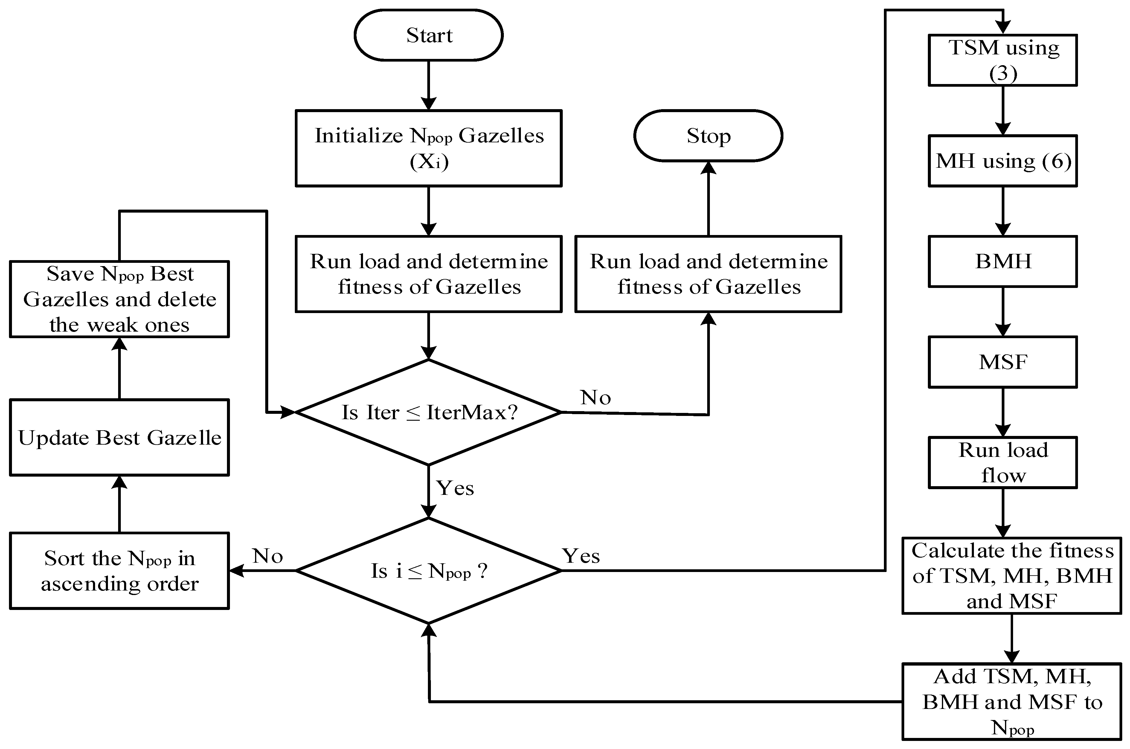
3.2. Application of MGO for DG Allocation

Computation Steps for Implementation of DG allocation using MGO are described in Figure 1. They are further discussed explicitly in the steps below:

• Step 1. Input the MGO parameters and distribution system line and load data
• Step 2. Initialize a random Npop population of Gazelles as given in Equation (32):

$$X={\left[\begin{array}{cccc}{X}_1& X_2& \dots & X_{N_{pop}}\end{array}\right]}^T$$

(32)

This denotes the population amount and represents the population’s gazelle. As expressed below, a gazelle is a potential solution comprising DG sizes, locations, and power factors:

$$X_i=\left[l_{DG,1} \dots l_{DG,n_{DG}}, S_{DG,1} \dots S_{DG,n_{DG}}, p{f}_{DG,1} \dots p{f}_{DG,n_{DG}}\right]$$

(33)

where $l_{DG,1}\dots l_{DG,n_{DG}}$ are the locations of the first to last DG installed on the RDN, $S_{DG,1}\dots S_{DG,n_{DG}}$ are the sizes or capacities of the first to the last DG installed on the RDN, $p{f}_{DG,1}\dots p{f}_{DG,n_{DG}}$ are the power factors of the first to the previous DG installed on the RDN, and $n_{DG}$ represents the amount of DGs installed on the RDN. During the initialization step, the solution variables for each gazelle are given random values inside their respective bounds in the manner described below:

$$l_{DG,n}=l_{DG,min}+rand\left(0,1\right)\times \left(l_{DG,\max }-l_{DG,\min }\right)$$

(34)

$$S_{DG,n}=S_{DG,min}+rand\left(0,1\right)\times \left(S_{DG,\max }-S_{DG,\min }\right)$$

(35)

$$p{f}_{DG,n}=p{f}_{DG,min}+rand\left(0,1\right)\times \left(p{f}_{DG,\max }-p{f}_{DG,\min }\right)$$

(36)

• Step 3. After selecting the DG type, perform load flow utilizing the Direct Load Flow (DLF) technique after modification of the line and load data for each initialized gazelle. Compute the fitness level and power loss of all the initialized gazelles as given in (37):

$$F_{fitness}=T{P}_{loss}+P_f{\displaystyle \sum _{K=1}^{K_n}{F}_K}$$

(37)

where $P_f$ is the penalty factor for different constraints $F_K$.

• Step 4. Set iter = 1
• Step 5. Utilize Equations (23), (28), (29) and (31) to determine TSM, MH, BMH, and MSF for each gazelle.
• Step 6. Determine the fitness and power loss of TSM, MH, BMH, and MSF by running load flow, then include them in the habitat.
• Step 7. Arrange the population as a whole in ascending order.
• Step 8. Adapt the fittest gazelle.
• Step 9. Store the N optimal gazelles in the maximum amount of populations
• Step 10. Increase Iter and go over Steps 5 to 9 if Iter is less than IterMax; if not, proceed to Step 11.
• Step 11. Present the optimal gazelle solution and compute the economic and technical assessments.

4. Results and Discussions

The developed approach was applied and validated on the standard 33-bus and 69-bus systems for the three cases, excluding the base case. The line and load data for the two RDNs can be seen in [37]. A thorough comparison with other known optimization methods is conducted to demonstrate the viability and efficacy of this improved approach. Each case is evaluated under three single, two, and three DG scenarios. The cases are as follows:

Case 0: Base case before changes due to DG penetration.

Case 1: Deployment of UPF DG using MGO.

Case 2: Deployment of FPF DG using MGO.

Case 3: Deployment of OPF DG using MGO.

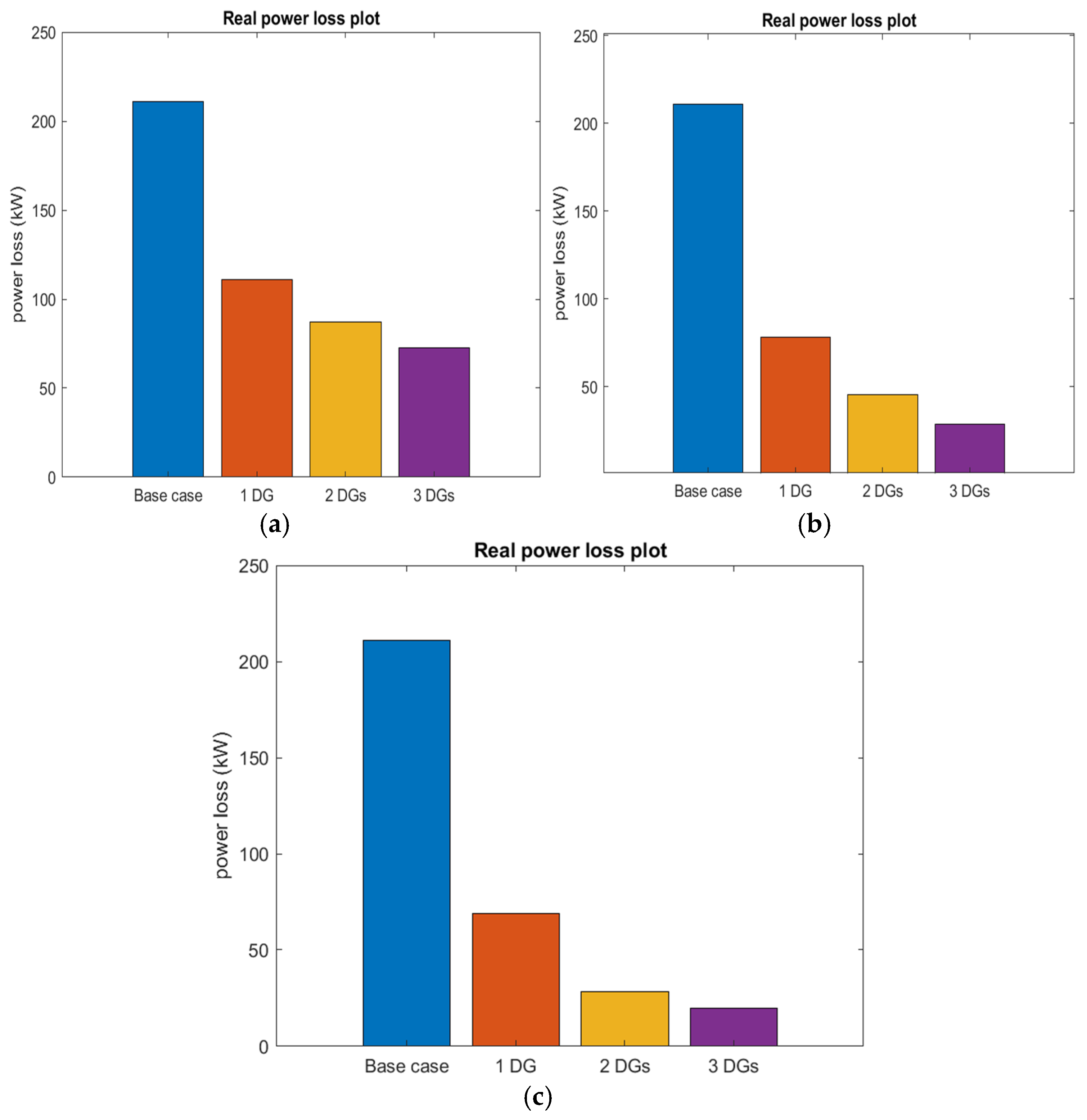
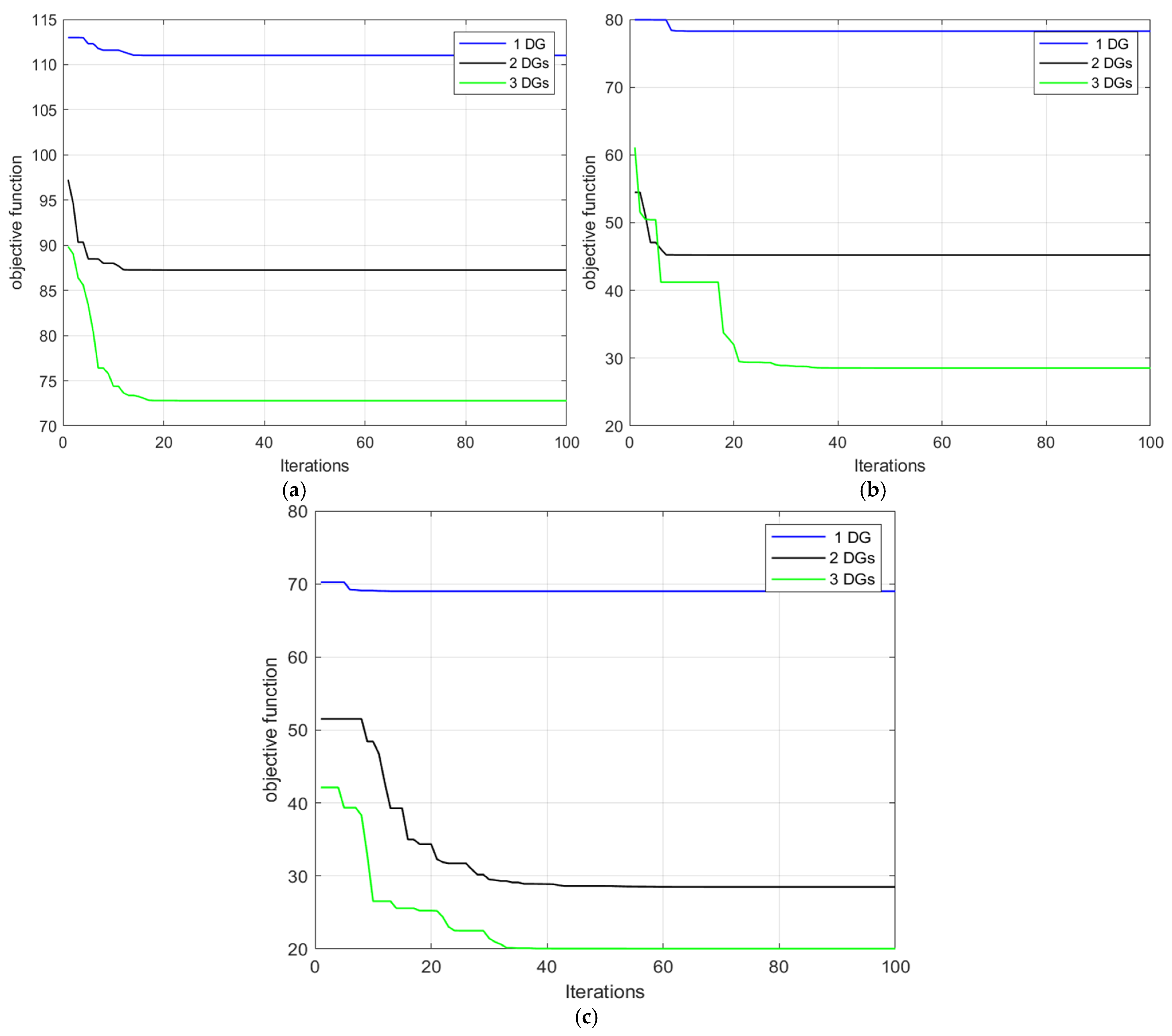
4.1. MGO Results for Standard 33-Bus RDN

4.1.1. Case One: Unity PF DGs

Table 1. Comparative result summary for case one (unity power factor DG).

Technique	Optimal DG			PL (kW)	%PL	VPI	V (p.u.)	Cost (USD)
	Location (Bus)	Size (kW)	Pf (p.u.)
Base Case				210.98		1.23	0.9038 (18)	CEL (USD) = 16,983.7877
Case One: One DG
GA [28]	2380 (6)			132.64	34.56
SFS [38]	2590 (6)			111.02	47.38
CSFS3 [38]	2590 (6)			111.02	47.38
CBOM [28]	2575 (6)			111.03	47.38
MGO	2590 (6)			111.02	47.38	1.54	0.9424 (18)	CEL (USD) = 8936.6326 PG-Cost ($/MWh) = 52.0500
Case Two: Two DGs
EA [39]	844 (13) 1149 (30)			87.17	58.68
EA-OPF [39]	852 (13) 1158 (30)			87.17	58.69
AM-PSO [40]	830 (13) 1110 (30)			87.28	58.64
SFS [38]	852 (13) 1158 (30)			87.17	58.69
CBOM [28]	852 (13) 1158 (30)			87.17	58.69
MGO	852 (13) 1157 (30)			87.17	58.69	1.68	0.9685 (33)	CEL (USD) = 7016.8101 PG-Cost ($/MWh) = 40.4300
Case Three: Three DGs
BFOA [26]	779 (14) 880 (25) 1083 (30)			73.53	65.14
QOSIMBO-Q [22]	771 (14) 1097 (24) 1096 (30)			72.79	65.49
SIMBO-Q [22]	764 (14) 1042 (24) 1135(29)			73.4	65.21
HHO [20]	746 (14) 1023 (24) 1136 (30)			72.98	65.40
IHHO [20]	776 (14) 1081 (24) 1067(30)			72.79	65.50
TSO [26]	772 (14) 1104 (24) 1065 (30)			72.79	65.50
SGA [30]	802 (13) 913 (24) 1054 (30)			72.79	65.50
ESGA [30]	771 (14) 1097 (24) 1066 (30)			72.79	65.50
ARO [32]	804 (13) 1094 (24) 1057 (30)			72.78	65.50
MGO	771 (14) 1097 (24) 1066 (30)			72.79	65.50	1.72	0.9687 (33)	CEL (USD) = 5859.2820 PG-Cost ($/MWh) = 58.9300

shows the outcomes of deploying DGs with UPF in the RDN. The algorithm provided a unity PF DG of 2590 kW capacity at bus 6 for a single DG allotment, corresponding to 111.02 kW and 81.72 kVAr for real and reactive power losses, respectively, also giving numerical values of VPI and minimum VSI as 1.92 and 0.92, respectively. Comparative analysis with the base case revealed a substantial reduction in real and reactive power losses, registering at 47.38% and 42.91%, respectively. The total CEL incurred was quantified at USD 936.6326. Further exploration involved the allocation of two DGs, each possessing a unity PF and capacities of 852 kW and 1157 kW at buses 13 and 30. This allocation manifested a considerable decrease in real and reactive power losses, yielding values of 87.17 kW and 59.81 kVAr, respectively, corresponding to 58.69% and 58.21% reduction in real and reactive power, respectively, also giving VPI and VSImin as 1.68 and 0.88. The CEL in the network for these two DGs amounted to USD 7016.8101. In analyzing the allocation of three DGs in the test network, the MGO algorithm exhibited significant results. Integrating DGs with capacities of 1097 kW, 771 kW, and 1066 kW at buses 24, 14, and 30, respectively, resulted in a substantial decrease in real and reactive power losses, measuring 72.79 kW and 50.72 kVAr, and presenting the VPI and VSImin to be 1.72 and 0.88, respectively. When contrasted with the base case, these reductions corresponded to 65.50% and 64.56% reductions. The cost of energy losses associated with this allocation was USD 5859.2820.

Comparative analysis across the three scenarios shows that the integration of three DGs yields a more favorable outcome for the objective function, highlighting substantial improvements in the test network with gradual increments in the DG units allocated.

4.1.2. Fixed PF DGs

Table 2. Comparative result summary for case two (0.95 FPF DG).

Technique	Optimal DG			PL (kW)	%PL	VPI	V (p.u.)	Cost (USD)
	Location (Bus)	Size (kW)	Pf (p.u.)
Base Case				210.98				CEL (USD) = 16,983.7877
Case One: One DG
MGO	2670 (6)		0.95	78.27	62.90	1.66	0.9547 (18)	CEL (USD) = 6300.3984 PG-Cost ($/MWh) = 53.6500 QG Cost ($/MVArh) = 2.5434
Case Two: Two DGs
MGO	13 30	840 1284	0.95 0.95	45.23	78.56	1.95	0.9798 (25)	CEL (USD) = 3640.8205 PG-Cost ($/MWh) = 42.7300 QG Cost ($/MVArh) = 2.0233
Case Three: Three DGs
QOSIMBO-Q [22]	13 24 30	830 1124 1240	0.95	28	86.49
SIMBO-Q [22]	13 24 30	888 1085 1309	0.95 0.95 0.95	29	86.26
HHO [20]	13 24 30	871 1327 1076	0.95 0.95 0.95	29.71	85.92
IHHO [20]	14 24 30	794 1132 1258	0.95 0.95 0.95	28.95	86.49
TSO [26]	13 24 30	833 1083 1250	0.95 0.95 0.95	28.50	86.49
ARO [32]	13 24 30	840 1138 1254	0.95 0.95 0.95	28.53	86.48
MGO	14 24 30	812 1080 1258	0.95 0.95 0.95	28.29	86.59	2.03	0.9880 (33)	CEL (USD) = 2296.5423 PG-Cost ($/MWh) = 60.9700 QG Cost ($/MVArh) = 2.8921

also provides detailed insights into the outcomes of integrating DGs with fixed power factors (0.95). In the case of a single DG allotment, the algorithm identified the optimal configuration as a 2841 kVA DG positioned at bus 6. This scenario yielded real and reactive power loss values, measuring 78.27 kW and 61.42 kVAr, respectively. The VPI and VSImin were obtained as 1.66 and 0.83, respectively. Compared with the base case, a noteworthy reduction in real and reactive power losses was demonstrated, registering at 62.90% and 57.09%, respectively. The quantified CEL associated with this single DG allocation amounted to USD 6300.3984. Subsequent exploration extended to allocating two DGs, each characterized by a fixed PF of 0.95, with capacities of 1352 kVA and 884 kVA at buses 30 and 13. This dual-DG allocation yielded effective reductions in real and reactive power losses, measuring 45.23 kW and 31.83 KVAr, respectively, 78.56% and 77.76% reductions and real and reactive power, respectively) and the obtained values of VPI and VSImin were 1.95 and 0.93, respectively. The cost of energy losses from allocating the two DGs was USD 3640.8205. Further analysis involved the allocation of three DGs within the test network. The MGO algorithm demonstrated significant outcomes, integrating DGs with capacities of 830 kVA, 1125 kVA, and 1240 kVA at buses 13, 24, and 30, respectively. This configuration resulted in substantial reductions in real and reactive power losses, measuring 28.53 kW and 21.21 kVAr, corresponding to 86.48% and 85.18% reductions, respectively, relative to the base case. The VPI and VSImin were also obtained as 2.03 and 0.95, respectively. The cost of energy losses associated with this three-DG allocation was USD 2296.5423. Finally, after comparing all three scenarios, the best outcomes for cost savings and power loss decrease were found when three DGs were integrated.

4.1.3. Variable PF DGs

Results from the optimal deployment of DGs with variable PFs in the test network are presented in

Table 3. Comparative result summary of case three (OPF DG).

Technique	Optimal DG			PL (kW)	%PL	VPI	Vmin (p.u.)	Cost (USD)
	Location (Bus)	Size (kW)	PF (p.u.)
Base Case				210.98		1.23	0.9038 (18)	CEL (USD) = 16,983.7877
Case One: One DG
CBOM [28]	26	2410		62.4	70.38
MGO	6	2423	0.82	60.03	72.28			CEL (USD) = 5556.6182 PG-Cost ($/MWh) = 39.9700 QGCost ($/MVArh) = 7.7812
Case Two: Two DGs
CBOM [28]	13 30	820 1243	0.8845 0.80	29.31	86.10
MGO	13 30	761 830	0.90 0.73	28.50	86.49	1.85	0.9803 (25)	CEL (USD) = 2294.1274 PG-Cost ($/MWh) = 32.3200 QG Cost ($/MVArh) = 6.9367
Case Three: Three DGs
HHO [20]	12 24 30	913 883 1079	0.85 0.82 0.83	14.94	92.92
IHHO [20]	14 24 30	762 1141 1014	0.90 0.91 0.71	11.83	93.39
TSO [26]	14 24 30	754 1143 1048	0.88 0.93 0.73	12.03	94.29
ARO [32]	13 24 30	807 1079 1031	0.91 0.91 0.72	11.74	94.44
SGA [30]	14 25 30	873 899 1459	0.903 0.939 0.6790	12.97	93.85
ESGA [30]	14 24 30	877 1188 1443	0.9050 0.9005 0.7133	11.74	94.44
MGO	13 24 30	385 492 994	0.8984 0.9100 0.7199	11.74	94.44	1.92	0.9825 (25)	CEL (USD) = 1613.1338 PG-Cost ($/MWh) = 41.2500 QGCost ($/MVArh) = 7.6870

. As returned by the algorithm, allocation of a single DG of capacity of 2423 kVA (0.82 PF) at bus six yields the optimal result, giving total real and reactive power losses of 60.03 kW and 55.23 kVAr, respectively, leading to 72.28% and 61.41% reduction relative to the base case. Calculations also returned values of 1.61 and 0.84 for the VPI and VSImin, respectively. The cost of energy losses obtained was quantified at USD 5 556.6182. Considering the allocation of two DGs, the algorithm returned optimal sizes of 846 kVA (0.90PF) and 1137kVA (0.73 PF) at buses 13 and 30, respectively, producing real and reactive power losses to the tune of 28.50 kW and 45 kVAr, respectively, corresponding to 86.49% and 85.73% real and reactive power loss reduction, respectively. The VPI and VSImin were 1.85 and 0.93, respectively. The CEL incurred amounted to USD 2294.1274. Moving on to the placement of three DGs in the DN, the optimal capacities of 646 kVA (0.91 PF), 991 kVA (0.87 PF), and 821 kVA (0.70 PF) at buses 14, 6, and 30 yielded 20.04 kW and 15.76 kVAr in real and reactive power losses, respectively, leading to a 90.50% and 88.99% reduction, respectively, when evaluated with the base case. The VPI and VSImin obtained were 1.92 and 0.94, respectively. The cost of energy losses obtained was USD 1613.1338. Eventually, comparing the three scenarios, it was observed that integration of three DGs in the system yielded loss diminution and percentage saved in cost.

4.1.4. Comparison of the Results Obtained from the Three Cases

Evaluating the results obtained from the study, it is observed that results sequentially got better with the increment in the amount of DG units for all scenarios, showcasing that the optimal DG units to be deployed in distribution networks to obtain the best results is 3. Moving on to the comparison between the three cases, it is worth noting that deploying DGs with variable power factors yielded the best results regarding percentage loss decrease and other parameters evaluated. An important point to also note from the simulation is that the performance of the networks increased sequentially with the gradual increase in the amount of DG units integrated into the networks for each scenario. Figure 2, Figure 3 and Figure 4 vividly compare the various simulated scenarios in terms of real power loss, voltage profile, and their respective convergence characteristics.

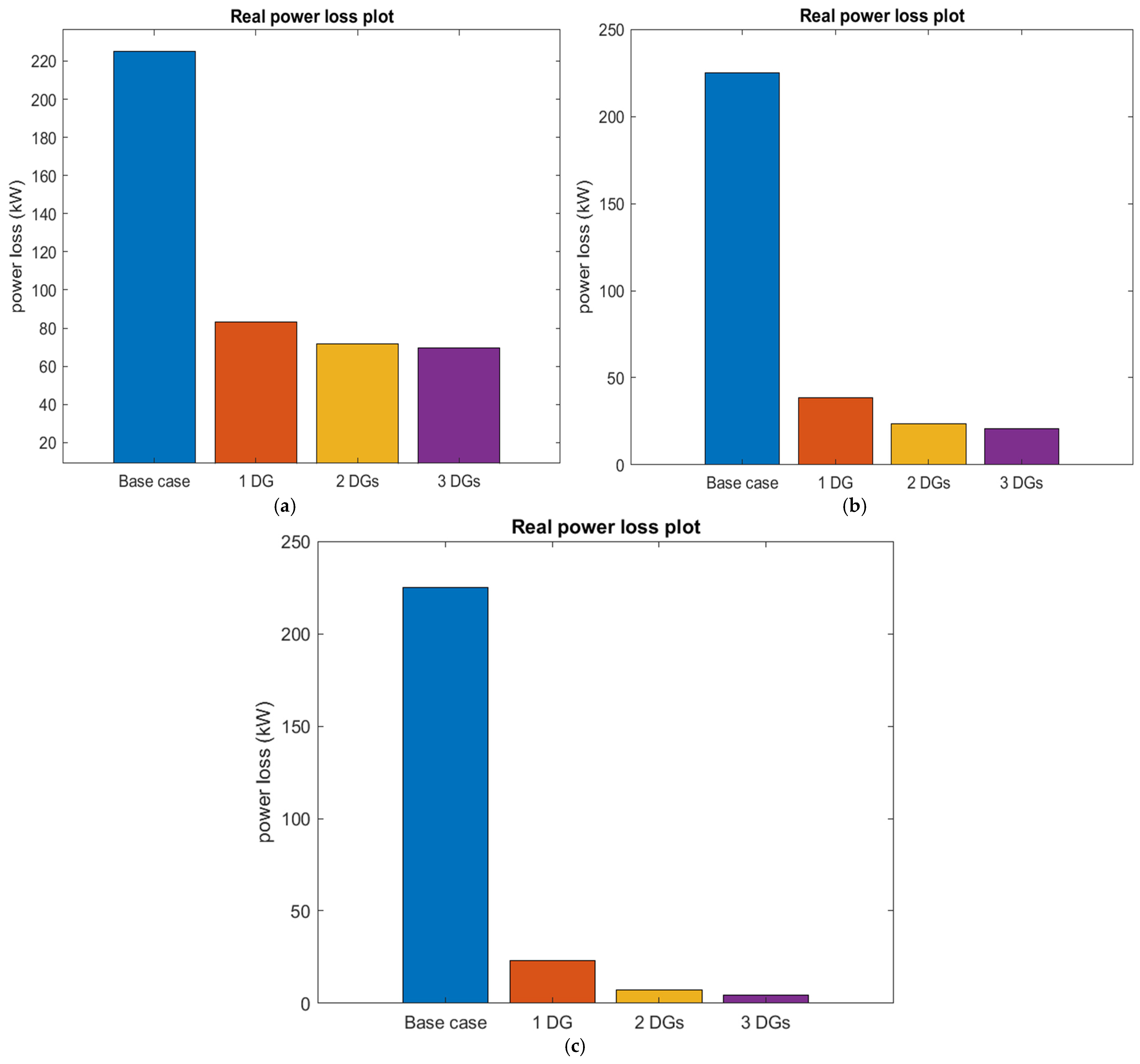
4.2. MGO Results for Standard IEEE 69-Bus System

4.2.1. Unity PF DGs

Table 4. Comparative result summary for case one (unity power factor DG).

Technique	Optimal DG			PL (kW)	%PL	VPI	V (p.u.)	Cost (USD)
	Location (Bus)	Size (kW)	pf (p.u.)
Base Case				210.98		1.23	0.9038 (18)	CEL (USD) = 18 110.7270
Case One: One DG
SFS [38]	1873 (61)			83.22	63.01
CSFS3 [38]	1873 (61)			83.22	63.01
CBOM [28]	1873 (61)			83.22	63.01
MGO	1873 (61)			83.22	63.01	1.89	0.9682 (27)	CEL (USD) = 6698.8521 PG-Cost ($/MWh) = 37.7100
Case Two: Two DGs
AGA [28]	389 (18) 1848 (61)			72.76	67.66
SFS [38]	531 (17) 1781 (61)			71.68	68.14
CSF3 [38]	531 (17) 1781 (61)			71.68	68.14
CBOM [28]	531 (17) 1781 (61)			71.68	68.14
MGO	532 (17) 1781 (61)			71.67	68.14	2.14	0.9789 (65)	CEL (USD) = 5769.1268 PG-Cost ($/MWh) = 46.5100
Case Three: Three DGs
TSO [26]	825 (9) 405 (22) 1650 (61)			70.25	68.77
QOSIMBO-Q [22]	834 (9) 480 (17) 1500 (61)			71.0	68.44
SIMBO-Q [22]	619 (9) 530 (17) 1500 (61)			71.3	68.31
HHO [20]	378 (11) 480 (17) 1706 (61)			69.73	69.00
IHHO [20]	527 (11) 382 (17) 1719 (61)			69.41	69.15
SGA [30]	467 (17) 1685 (54) 547 (53)			70.17	68.81
ABC [30]	576 (8) 1743 (61) 411 (17)			70.16	68.82
GA [30]	720 (50) 531 (17) 1781 (61)			70.16	68.82
MGO	1727 (18) 400 (18) 459 (66)			69.69	69.02	2.18	0.9790 (65)	CEL (USD) = 5609.7453 PG-Cost ($/MWh) = 51.9700

presents the results of the deployment of DGs with unity PF in the RDN. The algorithm provided a unity PF DG of 1873 kW capacity at bus 61 for a single DG allotment, corresponding to 83.22 kW and 40.53 kVAr for real and reactive power losses, respectively, also giving numerical values of VPI and minimum VSI as 1.89 and 0.88, respectively. Comparative analysis with the base case revealed a substantial decrease in real and reactive power losses, registering at 63.01 and 60.33%, respectively. The total cost incurred was quantified at USD 6698.8521. Further exploration involved the allocation of two DGs, each possessing a unity PF and capacities of 532 kW and 1781 kW at buses 17 and 61. This allocation manifested an effective reduction in real and reactive power losses, yielding values of 71.67 kW and 35.94 kVAr, respectively, corresponding to 68.14% and 65.68% reduction in real and reactive power, respectively, also giving VPI and VSImin as 2.14 and 0.92. The total cost of energy losses for these two DGs amounted to USD 5769.1268. In the third scenario, expanding the analysis to the allocation of three DGs in the test network, the MGO algorithm exhibited significant results. Integrating DGs with capacities of 1727 kW, 400 kW, and 459 kW at buses 61, 18, and 66, respectively, resulted in a considerable decrease in real and reactive power losses, measuring 69.69 kW and 35.06 kVAr, and presenting the VPI and VSImin to be 2.18 and 0.92, respectively. When contrasted with the base case, these reductions corresponded to 69.02% and 65.68% reductions. The cost of energy losses associated with this allocation was USD 5609.7453.

Comparative analysis across the three scenarios underscores that integrating three DGs yields a more favorable outcome for the objective function, specifically the diminution of power loss. This observation emphasizes the optimal deployment of DGs in an RDN to achieve desired operational objectives.

4.2.2. Fixed PF DGs

Table 5. Comparative result summary for case two (0.95 FPF DG).

Technique	Optimal DG			PL (kW)	%PL	VPI	V (p.u.)	Cost (USD)
	Location (Bus)	Size (kW)	Pf (p.u.)
Base Case				210.98		1.56	0.9092 (65)	CEL (USD) = 18,110.7270
Case One: One DG
MGO	61	1947	0.95	38.41	82.93	2.00	0.9717 (27)	CEL (USD) = 3091.8398 PG-Cost ($/MWh) = 39.1900 QGCost ($/MVArh) = 1.8547
Case Two: Two DGs
MGO	61 17	1849 550	0.95 0.95	23.48	89.56	2.44	0.9934 (69)	CEL (USD) = 1890.0390 PG-Cost ($/MWh) = 48.2300 QGCost ($/MVArh) = 2.2853
Case Three: Three DGs
TSO [26]	11 18 61	352 501 1878	0.95 0.95 0.95	21.13	90.61
SIMBO-Q [22]	19 61 64	566 1500 422	0.95 0.95 0.95	23.1	89.73
QOSIMBO-Q [22]	17 61 64	583 1500 427	0.95 0.95 0.95	22.80	89.87
HHO [20]	16 50 61	703 287 1891	0.95 0.95 0.95	22.85	89.80
IHHO [20]	11 18 61	5533 420 1879	0.95 0.95 0.95	20.71	90.80
MGO	21 61 11	361 178 567	0.95 0.95 0.95	20.73	90.79	2.56	0.9942 (50)	CEL (USD) = 1668.6758 PG-Cost ($/MWh) = 54.4700 QG-Cost ($/MVArh) = 2.5825

also provides detailed insights into the outcomes of integrating Ds with fixed power factors (0.95). In the case of a single DG allotment, the algorithm identified the optimal configuration as a 2049 kVA DG positioned at bus 61. The novel algorithm yielded real and reactive power loss values, measuring 38.41 kW and 21.00 kVAr, respectively. The VPI and VSImin were obtained as 2.00 and 0.89, respectively. Compared with the base case, a noteworthy reduction in real and reactive power losses was observed, registering at 82.93% and 79.44%, respectively. The quantified cost of energy losses associated with this single DG allocation amounted to USD 3091.8398. Subsequent exploration extended to allocating two DGs, each characterized by a fixed PF of 0.95, with capacities of 1946 kVA and 579 kVA at buses 61 and 17. This scenario of dual-DG allocation yielded effective reductions in real and reactive power losses, measuring 23.48 kW and 15.09 kVAr, respectively, (89.56% and 85.23% reductions and real and reactive power, respectively), and the obtained values of VPI and VSImin are 2.44 and 0.97, respectively. The total cost obtained from allocating the two DGS was USD 1890.0390.

Further analysis involved the allocation of three DGs within the test network. The MGO algorithm demonstrated significant outcomes, integrating DGs with capacities of 361 kVA, 1877 kVA, and 597 kVA at buses 21, 61, and 11, respectively. This configuration resulted in substantial reductions in real and reactive power losses, measuring 20.73 kW and 13.89 kVAr, corresponding to 90.79% and 86.41% reductions, respectively, relative to the base case. The VPI and VSImin were also obtained as 2.56 and 0.98, respectively. The total cost associated with this three-DG allocation was USD 1668.6758. Finally, comparing all three scenarios, the best outcomes in terms of cost savings and power loss decrease were found when three DGs were integrated

4.2.3. Variable PF DGs

Results from the optimal integration of DGs with variable PFs in the test network are also presented in

Table 6. Comparative result summary for case three (OPF DG).

Technique	Optimal DG			PL (kW)	%PL	VPI	V (p.u.)	Cost (USD)
	Location (Bus)	Size (kW)	Pf (p.u.)
Base Case				210.98		1.56	0.9092 (65)	CEL (USD) = 18,110.7270
Case One: One DG
BB-BC [28]	61	1801	0.81	23.17	89.69
ALOA [41]	61	1827	0.82	23.19	89.69
CBOM [28]	61	1828	0.81	23.17	89.70
MGO	61	1849	0.81	23.17	89.70	1.93	0.9725 (27)	CEL (USD) = 1865.0854 PG-Cost ($/MWh) = 30.0300 QGCost ($/MVArh) = 6.2264
Case Two: Two DGs
ALOA [41]	17 61	603 1200	0.83 0.80	20.93	90.69
CBOM [28]	17 61	522 1735	0.83 0.81	7.20	96.79
MGO	61 17	1412 432	0.81 0.83	7.20	96.80	2.21	0.9943 (50)	CEL (USD) = 579.5690 PG-Cost ($/MWh) = 37.3800 QGCost ($/MVArh) = 7.4856
Case Three: Three DGs
TSO [26]	12 59 61	697 846 1064	0.80 0.91 0.81	11.89	94.71
HHO [20]	17 61 66	271 1541 697	0.57 0.76 0.97	6.58	97.10
IHHO [20]	11 18 61	456 389 1715	0.85 0.82 0.83	4.44	98.00
ESGA [30]	18 61 11	378 1672 494	0.83 0.81 0.81	4.27	98.10
SGA [30]	61 19 11	1681 386 439	0.82 0.87 0.71	4.36	98.06
ABC [30]	61 18 66	1791 323 417	0.81 0.87 0.71	4.98	97.79
MGO	18 11 61	320 391 1365	0.84 0.80 0.81	4.27	98.10	2.27	0.9943 (50)	CEL (USD) = 343.7166 PG-Cost ($/MWh) = 42.2700 QGCost ($/MVArh) = 8.5387

. As returned by the algorithm, allocation of a single DG of the capacity of 1828 kVA (0.81 PF) at bus 61 yields the optimal result, giving total real and reactive power losses of 23.17 kW and 14.37 kVAr, respectively, leading to an 89.70% and 85.93% reduction when relative to the base case. Calculations also returned values of 1.93 and 0.89 for the VPI and VSImin, respectively. The cost of energy losses obtained was quantified at USD 1865.0854. Considering the allocation of two DGs, the algorithm returned optimal sizes of 1735 kVA (0.81 PF) and 1137 kVA (0.83 PF) at buses 61 and 17, respectively, producing real and reactive power losses to the tune of 7.20 kW and 8.04 kVAr, respectively, corresponding to 96.80% and 92.13% real and reactive power loss reduction. The VPI and VSImin were 2.21 and 0.98, respectively. The CEL incurred amounted to USD 579.5690. Moving on to the deployment of three DGs in the DN, the optimal capacities of 382 kVA (0.84 PF), 486 kVA (0.80 PF), and 1676 kVA (0.81 PF) at buses 18, 11, and 61 yielded 4.27 kW and 6.75 kVAr in real and reactive power losses, respectively, leading to a 98.10% and 93.38% reduction, respectively, when evaluated with the base case. The VPI and VSImin obtained were 2.27 and 0.98, respectively. The cost of energy losses obtained was USD 343.7166. Eventually, comparing the three scenarios, it was found that the inclusion of three DGs in the system led to the best results regarding loss reduction and value saved in cost.

4.2.4. Comparison of the Results Obtained from the Three Test Cases

Evaluating the results obtained from the study, it is observed that results sequentially got better with the increment in the amount of DG units for all scenarios, showcasing that the optimal DG units to be deployed in RDN to obtain the best results is 3. Moving on to the comparison between the three cases, it is worth noting that deploying DGs with variable power factors yielded the best results regarding percentage loss decrease and other parameters evaluated. An important point to also note from the simulation is that the performance of the networks increased sequentially with the gradual increase in the amount of DG units integrated into the networks for each scenario. Figure 5, Figure 6 and Figure 7 vividly compare the various simulated scenarios regarding real power loss, voltage profile, and their convergence characteristics.

5. Conclusions

This research presents a comprehensive analysis of the Mountain Gazelle Optimizer (MGO) for the optimal deployment of distributed generators (DGs) in radial distribution networks (RDNs). The study effectively addresses the gap regarding integrating DGs with variable power factors, showcasing the significant impact of power factor optimization on reducing power losses and enhancing the overall performance of RDNs. Through simulations on the IEEE 33-bus and 69-bus systems, the MGO demonstrated superior efficiency in minimizing real and reactive power losses compared to existing optimization techniques. The results indicate that the performance of RDNs improves correspondingly with the increments in the number of integrated DG units, demonstrating substantial reductions in energy losses and improved voltage stability and profile. Additionally, it was determined that deploying DGs with optimal power factor achieved the best results in terms of the set-out objectives. Furthermore, the economic implications of optimal DG placement were evaluated, highlighting the potential for significant cost savings through reduced energy losses. This research enhances understanding of DG allocation theoretically and provides actionable insights for boosting power system reliability and sustainability. However, it is to be noted that this work, through simulations, mainly focused on showcasing how the variation in DG power factor can impact the power loss and the cost efficiency of a distribution network. Building on this, future works can look into the practical implementation of this technique, especially in developing countries. For example, developing a real-time current, voltage, and power measuring system in the network for the efficient integration of the OPF DGs. Additionally, for the efficient, stable, and coordinated operation of the integrated DGs within a large electrical network, future work can also explore developing a central coordinator that will be typically employed to optimize the power factor settings of individual generators to meet system-wide objectives. Furthermore, future work could also investigate the application of MGO for optimizing DG deployment in unbalanced distribution networks with three-phase loads. Likewise, this optimization methodology can be utilized in optimizing systems with objective functions centered on environmental benefits by utilizing DGs with renewable sources, thereby further advancing the field of distributed generation optimization.

References

1. Prakash, K.; Lallu, A.; Islam, F.R.; Mamun, K.A. Review of Power System Distribution Network Architecture. In Proceedings of the 2016 3rd Asia-Pacific World Congress on Computer Science and Engineering (APWC on CSE), Nadi, Fiji, 5–6 December 2016; pp. 124–130. [Google Scholar] [CrossRef]
2. Shi, S.; Zhu, B.; Lei, A.; Dong, X. Fault location for radial distribution network via topology and reclosure-generating traveling waves. IEEE Trans. Smart Grid 2019, 10, 6404–6413. [Google Scholar] [CrossRef]
3. Duppala, D.; Nagaballi, S.; Kale, V.S. The Technical Impact of Increase in Penetration Level of DG Technologies on Power System. In Proceedings of the of 2019 IEEE Region 10 Symposium (TENSYMP), Kolkata, India, 7–9 June 2019; pp. 491–496. [Google Scholar] [CrossRef]
4. Paliwal, P.; Patidar, N.P.; Nema, R.K. Planning of grid integrated distributed generators: A review of technology, objectives and techniques. Renew. Sustain. Energy Rev. 2014, 40, 557–570. [Google Scholar] [CrossRef]
5. Huy, T.H.B.; Tran, T.; Van Tran, T.; Vo, D.N.; Nguyen, H.T.T. An improved metaheuristic method for simultaneous network reconfiguration and distributed generation allocation. Alex. Eng. J. 2022, 61, 8069–8088. [Google Scholar] [CrossRef]
6. Salimon, S.A.; Adepoju, G.A.; Adebayo, I.G.; Howlader, H.O.R.; Ayanlade, S.O.; Adewuyi, O.B. Impact of Distributed Generators Penetration Level on the Power Loss and Voltage Profile of Radial Distribution Networks. Energies 2023, 16, 1943. [Google Scholar] [CrossRef]
7. Lalitha, M.P.; Reddy, V.C.V.; Reddy, N.S.; Reddy, V.U. DG Source Allocation by Fuzzy and Clonal Selection Algorithm for Minimum Loss in Distribution System. Distrib. Gener. Altern. Energy J. 2011, 26, 17–35. [Google Scholar] [CrossRef]
8. Hung, D.Q.; Mithulananthan, N. Multiple Distributed Generator Placement in Primary Distribution Networks for Loss Reduction. IEEE Trans. Ind. Electron. 2013, 60, 1700–1708. [Google Scholar] [CrossRef]
9. El-Fergany, A. Optimal allocation of multi-type distributed generators using backtracking search optimization algorithm. Int. J. Electr. Power Energy Syst. 2015, 64, 1197–1205. [Google Scholar] [CrossRef]
10. Moradi, M.H.; Abedini, M. A novel method for optimal DG units capacity and location in Microgrids. Int. J. Electr. Power Energy Syst. 2016, 75, 236–244. [Google Scholar] [CrossRef]
11. ChithraDevi, S.A.; Lakshminarasimman, L.; Balamurugan, R. Stud Krill herd Algorithm for multiple DG placement and sizing in a radial distribution system. Eng. Sci. Technol. Int. J. 2017, 20, 748–759. [Google Scholar] [CrossRef]
12. Meena, N.K.; Swarnkar, A.; Gupta, N.; Niazi, K.R. Multi-objective Taguchi approach for optimal DG integration in distribution systems. IET Gener. Transm. Distrib. 2017, 11, 2418–2428. [Google Scholar] [CrossRef]
13. Selim, A.; Kamel, S.; Jurado, F. Efficient optimization technique for multiple DG allocation in distribution networks. Appl. Soft Comput. 2020, 86, 105938. [Google Scholar] [CrossRef]
14. Balu, K.; Mukherjee, V. Optimal siting and sizing of distributed generation in radial distribution system using a novel student psychology-based optimization algorithm. Neural Comput. Appl. 2021, 33, 15639–15667. [Google Scholar] [CrossRef]
15. Ali, M.H.; Kamel, S.; Hassan, M.H.; Tostado-Véliz, M.; Zawbaa, H.M. An improved wild horse optimization algorithm for reliability based optimal DG planning of radial distribution networks. Energy Rep. 2022, 8, 582–604. [Google Scholar] [CrossRef]
16. Sellami, R.; Farooq, S.H.E.R.; Rafik, N.E.J.I. An improved MOPSO algorithm for optimal sizing & placement of distributed generation: A case study of the Tunisian offshore distribution network (ASHTART). Energy Rep. 2022, 8, 6960–6975. [Google Scholar]
17. Subbaramaiah, K.; Sujatha, P. Optimal DG unit placement in distribution networks by multi-objective whale optimization algorithm & its techno-economic analysis. Electr. Power Syst. Res. 2023, 214, 108869. [Google Scholar]
18. Gümüş, T.E.; Emiroglu, S.; Yalcin, M.A. Optimal DG allocation and sizing in distribution systems with Thevenin based impedance stability index. Int. J. Electr. Power Energy Syst. 2023, 144, 108555. [Google Scholar] [CrossRef]
19. Purlu, M.; Turkay, B.E. Optimal Allocation of Renewable Distributed Generations Using Heuristic Methods to Minimize Annual Energy Losses and Voltage Deviation Index. IEEE Access 2022, 10, 21455–21474. [Google Scholar] [CrossRef]
20. Shadman Abid, M.; Apon, H.J.; Morshed, K.A.; Ahmed, A. Optimal Planning of Multiple Renewable Energy-Integrated Distribution System with Uncertainties Using Artificial Hummingbird Algorithm. IEEE Access 2022, 10, 40716–40730. [Google Scholar] [CrossRef]
21. Selim, A.; Kamel, S.; Alghamdi, A.S.; Jurado, F. Optimal placement of DGs in distribution system using an improved harris hawks optimizer based on single-and multi-objective approaches. IEEE Access 2020, 8, 52815–52829. [Google Scholar] [CrossRef]
22. Sultana, S.; Roy, P.K. Multi-objective quasi-oppositional teaching learning-based optimization for optimal location of distributed generator in radial distribution systems. Int. J. Electr. Power Energy Syst. 2014, 63, 534–545. [Google Scholar] [CrossRef]
23. Sharma, S.; Bhattacharjee, S.; Bhattacharya, A. Quasi-Oppositional Swine Influenza Model Based Optimization with Quarantine for optimal allocation of DG in radial distribution network. Int. J. Electr. Power Energy Syst. 2016, 74, 348–373. [Google Scholar] [CrossRef]
24. Salimon, S.A.; Adepoju, G.A.; Adebayo, I.G.; Adewuyi, O.B. Comparative assessment of techno-economic and environmental benefits in optimal allocation of distributed generators in distribution networks. Sci. Afr. 2023, 19, e01546. [Google Scholar] [CrossRef]
25. Adebiyi, O.W.; Okelola, M.O.; Salimon, S.A. Multi-objective Optimal Allocation of Renewable Energy Distributed Generations and Shunt Capacitors in Radial Distribution System using Corona Virus Herd Optimization. Majlesi J. Electr. Eng. 2023. [Google Scholar]
26. Bhadoriya, J.S.; Gupta, A.R. A novel transient search optimization for optimal allocation of multiple distributed generator in the radial electrical distribution network. Int. J. Emerg. Electr. Power Syst. 2022, 23, 23–45. [Google Scholar] [CrossRef]
27. Nguyen, T.P.; Vo, D.N. A novel stochastic fractal search algorithm for optimal allocation of distributed generators in radial distribution systems. Appl. Soft Comput. 2018, 70, 773–796. [Google Scholar] [CrossRef]
28. Memarzadeh, G.; Arabzadeh, M.; Keynia, F. A new optimal allocation of DGs in distribution networks by using coot bird optimization method. Energy Inform. 2023, 6, 30. [Google Scholar] [CrossRef]
29. Pham, T.D.; Nguyen, T.T.; Dinh, B.H. Find optimal capacity and location of distributed generation units in radial distribution networks by using enhanced coyote optimization algorithm. Neural Comput. Appl. 2021, 33, 4343–4371. [Google Scholar] [CrossRef]
30. Huy, T.H.B.; Vo, D.N.; Truong, K.H.; Van Tran, T. Optimal Distributed Generation Placement in Radial Distribution Networks using Enhanced Search Group Algorithm. IEEE Access 2023, 11, 103288–103305. [Google Scholar] [CrossRef]
31. Iftikhar, M.Z.; Imran, K.; Akbar, M.I.; Ghafoor, S. Optimal distributed generators allocation with various load models under load growth using a meta-heuristic technique. Renew. Energy Focus 2024, 49, 100550. [Google Scholar] [CrossRef]
32. Sharma, R.K.; Naick, B.K. A Novel Artificial Rabbits Optimization Algorithm for Optimal Location and Sizing of Multiple Distributed Generation in Radial Distribution Systems. Arab. J. Sci. Eng. 2024, 49, 6981–7012. [Google Scholar] [CrossRef]
33. Abdollahzadeh, B.; Gharehchopogh, F.S.; Khodadadi, N.; Mirjalili, S. Mountain gazelle optimizer: A new nature-inspired metaheuristic algorithm for global optimization problems. Adv. Eng. Softw. 2022, 174, 103282. [Google Scholar] [CrossRef]
34. Salimon, S.A.; Adepoju, G.A.; Adebayo, I.G.; Ayanlade, S.O. Impact of shunt capacitor penetration level in radial distribution system considering techno-economic benefits. Niger. J. Technol. Dev. 2022, 19, 101–109. [Google Scholar] [CrossRef]
35. Adepoju, G.A.; Salimon, S.A.; Adebayo, I.G.; Adewuyi, O.B. Impact of DSTATCOM penetration level on technical benefits in radial distribution network. e-Prime-Adv. Electr. Eng. Electron. Energy 2024, 7, 100413. [Google Scholar] [CrossRef]
36. Kashyap, M.; Kansal, S.; Verma, R. Sizing and allocation of DGs in a passive distribution network under various loading scenarios. Electr. Power Syst. Res. 2022, 209, 108046. [Google Scholar] [CrossRef]
37. Taher, S.A.; Karimi, M.H. Optimal reconfiguration and DG allocation in balanced and unbalanced distribution systems. Ain Shams Eng. J. 2014, 5, 735–749. [Google Scholar] [CrossRef]
38. Nguyen, T.P.; Tran, T.T.; Vo, D.N. Improved stochastic fractal search algorithm with chaos for optimal determination of location, size, and quantity of distributed generators in distribution systems. Neural Comput. Appl. 2019, 31, 7707–7732. [Google Scholar] [CrossRef]
39. Mahmoud, K.; Yorino, N.; Ahmed, A. Optimal distributed generation allocation in distribution systems for loss minimization. IEEE Trans. Power Syst. 2015, 31, 960–969. [Google Scholar] [CrossRef]
40. Kansal, S.; Kumar, V.; Tyagi, B. Hybrid approach for optimal placement of multiple DGs of multiple types in distribution networks. Int. J. Electr. Power Energy Syst. 2016, 75, 226–235. [Google Scholar] [CrossRef]
41. Ali, E.S.; Abd Elazim, S.M.; Abdelaziz, A.Y. Ant Lion Optimization Algorithm for optimal location and sizing of renewable distributed generations. Renew. Energy 2017, 101, 1311–1324. [Google Scholar] [CrossRef]
Figure 1. Flowchart for application of MGO for DG allocation.
Technologies 13 00265 g001
Figure 2. Comparative loss plot for all scenarios on the standard 33-bus RDN; (a) unity PF DGs; (b) fixed PF DGs; (c) optimal/variable PF DGs.
Technologies 13 00265 g002
Figure 3. Comparative bus voltage plot for the standard 33-bus system (a) unity PF DGs; (b) fixed PF DGs; (c) optimal/variable PF DGs.
Technologies 13 00265 g003
Figure 4. Comparative convergence curve characteristics for the standard 33-bus system (a) unity PF DGs; (b) fixed PF DGs (c) optimal/variable PF DGs.
Technologies 13 00265 g004
Figure 5. Comparative loss plot for the standard 69-bus system (a) unity PF DGs; (b) fixed PF DGs; (c) optimal/variable PF DGs.
Technologies 13 00265 g005
Figure 6. Comparative voltage plot on the standard 69-bus network (a) unity PF DGs; (b) fixed PF DGs; (c) optimal/variable PF DGs.
Technologies 13 00265 g006
Figure 7. Comparative convergence curve for the standard 69-bus system (a) unity PF DGs (b); fixed PF DGs; (c) optimal/variable PF DG.
Technologies 13 00265 g007