Center of Mass Auto-Location in Space ^†

Abstract

Maintaining a spacecraft’s center of mass at the origin of a body-fixed coordinate system is often key to precision trajectory tracking. Typically, the inertia matrix is estimated and verified with preliminary ground testing. This article presents groundbreaking preliminary results and significant findings from on-orbit space experiments validating recently proposed methods as part of a larger study over multiple years. Time-varying estimates of inertia moments and products are used to reveal time-varying estimates of the location of spacecraft center of mass using geosynchronous orbiting test satellites proposing a novel two-norm optimal projection learning method. Using the parallel axis theorem, the location of the mass center is parameterized using the cross products of inertia, and that information is extracted from spaceflight maneuver data validating modeling and simulation. Mass inertia properties are discerned, and the mass center is experimentally revealed to be over thirty centimeters away from the assumed locations in two of the three axes. Rotation about one axis is found to be very well balanced, with the center of gravity lying on that axis. Two-to-three orders of magnitude corrections to inertia identification are experimentally demonstrated. Combined-axis three-dimensional maneuvers are found to obscure identification compared with single-axis maneuvering as predicted by the sequel analytic study. Mass center location migrates 36–95% and subsequent validating experiments duplicate the results to within 0.1%.

1. Introduction

Figure 1. Communication links in and from space. (a) The Space Development Agency (SDA) received approval from the International Telecommunication Union (ITU) for experimental use of Link 16 from space using radios flown on the Tranche 0 Transport satellites. Image credit: SDA [1], used in accordance with image use policy; [2] (b) Air Force Research Laboratory (AFRL) XVI satellite, host of Link 16 payload [3].

Figure 1. Communication links in and from space. (a) The Space Development Agency (SDA) received approval from the International Telecommunication Union (ITU) for experimental use of Link 16 from space using radios flown on the Tranche 0 Transport satellites. Image credit: SDA [1], used in accordance with image use policy; [2] (b) Air Force Research Laboratory (AFRL) XVI satellite, host of Link 16 payload [3].

Earth-orbiting spacecraft (e.g., Figure 1) often waste fuel due to correcting trajectory tracking errors due to mass imbalance, shortening their mission lifecycles. Amelioration holds promise of substantial savings. In the remainder of this section of this article, the current state of the research field is reviewed, and key publications are cited. Controversial and diverging hypotheses are introduced. Finally, the main aim of this work is briefly mentioned, and the principal conclusions are highlighted after foremostly introducing the general problem statement.

• Problem Statement: Generally, inertia moments are estimated on the ground, while some recent attempts have been made to estimate them on an orbit. The estimation of inertia products is relatively rare, despite the ability to parameterize the location of the mass center using the parallel axis theorem. This study elaborates a novel process for determining the time-varying location of the mass center on orbit by using the parallel axis theorem to parameterize the problem and then estimating the time-varying inertia properties leads to the auto-location of the spacecraft’s center of mass.
• Research objectives: (1) Using only attitude empirical angle knowledge, find mass imbalanced inertia components and (2) convert mass imbalance to center of gravity coordinates, and then calculate that location.
• Key contributions: Seminal proposal of a novel mass center auto-location method is introduced, realizing improvements over the comparative state-of-the-art benchmark. Rapid convergence is validated in spaceflight experiments.

1.1. Review of the Literature

One mission context for the center of mass auto-location is grappling space robotics (e.g., Figure 2), and the U.S. Naval Academy provides a worthy benchmark launched into space in December 2018. Two 3D-printed manipulator arms are attached to the RSAT–P (USNA–19) cubesat on the NASA ELaNa XIX space mission.

Such robotic space missions necessitate autonomous knowledge of mass properties in situ, and many approaches have appeared in the recent literature. A very recent proposal includes using an extended Kalman filter combined with a Rauch–Tung–Striebel smoother was used to estimate the offset, where the chi-square test was used to eliminate outliers, where a slightly improved performance was achieved detecting gravitational waves [5]. Laser range finders are one ubiquitous system used to locate the center of mass on orbit. Center of mass values used for Ajisai geodetic satellites using satellite laser ranging relied on [6], the work of Otsubo and Appleby. These values have been superseded by the relatively new work described in [7], which revealed that a major contributor to the error budget in satellite laser ranging (SLR) for reference frame realization has been a limited accuracy of the CoM corrections The new values [7] can result in a roughly twenty millimeter change for big targets compared with earlier modeling [6], where the study also concluded that standard center of mass corrections yield inaccurate on-orbit solutions. The latest corrections are presented in [8]. The concept of corrections is depicted in Figure 3.

The center of mass correction using laser ranging data was also employed by the CHAMP satellite [11], the Etalon-1 and -2 satellites [12], Galileo-101 and -102 satellites [13], and U.S. Navy GEOSAT spacecraft [14].

Correction may be accomplished using a set of three internal shifting masses (ISMs) that can be displaced and a mass estimation method based in the recursive least squares algorithm claiming “…a convergence of an acceptable value of the position of the center of mass of the satellite in approximately 120 s, while the relative error is less than 5%” [15]. The method proposed in this manuscript is similar to the method proposed in [15], but merely topically. The latter technique uses recursive least squares to estimate the location, while the presently proposed method uses a novel 2-norm optimal estimator to produce values for inertia moments and products (useful within themselves) and then the inertia products (only) are used to directly calculate the mass center location by accepting parameterization using the parallel axis theorem. The latter method (from reference [15]) yields initial rapid convergence, then divergence before stabilizing with a finite, but noticeable offset. In 2021, optimization of mass center location was proposed using linear means, incrementally adding environmental disturbances as constraints and then optimizing component mass locations [16].

More recently, inflight estimation of the position of the center of gravity was elaborated using arrays of accelerometers [17]. Integer programming models were proposed for accurate center of gravity control in [18]. An integrated estimation approach sequentially combined a Huber-extended Kálmán filter and extended Kálmán filter to estimate the center of gravity location. The Huber version of the filter is used first to find the estimated distance between a vehicle’s front axle and the center of gravity, while the extended filter locates the center of gravity with a claimed performance of a two percent estimation error within two seconds [19]. Similar to the comments in the preceding paragraph’s comparison of the methods in reference [15], the methods proposed in [19] are similar topically, but quite different than the methods presently proposed. The methods in reference [19] propose using Kalman filtering methods for state estimation (particularly velocity), then Huang modeling to estimate the mass center, while the presently proposed methods use a novel two-norm optimal estimator for the inertia components (moments and products), then uses the products to directly calculate the mass center location by accepting parameterization using the parallel axis theorem. Meanwhile, [20] integrated observers for real-time estimation of the height of the mass center. Reference [21] proposed combining an adaptive Kálmán filter and extended Kálmán filter to estimate mass center location and particularly focused on persistence of excitation. H∞ methods (used in control theory to synthesize controllers to achieve stabilization with guaranteed performance) and the extended Kálmán filter joint estimation method was used to determine the mass center position in [22]. Adaptive online estimation was proposed in [23] for height location only of the mass center.

Feedback linearizing control was used in [24] to account for time-varying mass center location during spacecraft orbital refueling.

The historical approaches described generally fall into two categories: accelerometer sensing to utilize first principles for estimation or alternatively filtering approaches. Meanwhile, some novel approaches have been recently suggested.

1.2. State-of-the-Art Benchmarks

The following list highlights the current developing state-of-the art deterministic artificial intelligence (“deterministic AI systems operate under the principle that every set of particular conditions will always lead to the same outcome” [25]):

• Mass center coordinate estimation based on an overall brightness average determined from a three-dimensional vision system [26].
• Reference [27] presents an exact analytic method for calculating the volume, mass, center of gravity, and inertia properties of wing segments and rotors of constant density, emphasizing analysis requiring the analytical solution of several volume integrals (necessarily a quite lengthy process). The goal of this present study is akin to this state-of-the-art benchmark, while avoiding such complications.
• Reference [28] combines multiple accelerometers and gyroscopes into an inertial measurement unit mounted on the pitch and yaw axes, where the roll axis houses the gyroscope used to determine the spin axis.
• References [29,30] proposed a novel approach to use any attitude maneuver to analytically find the location of the mass center necessitating nonlinear enhanced Luenberger observers to estimate the constituent variables, permitting angle data alone to yield mass center location estimates.

1.3. Novelties Presented

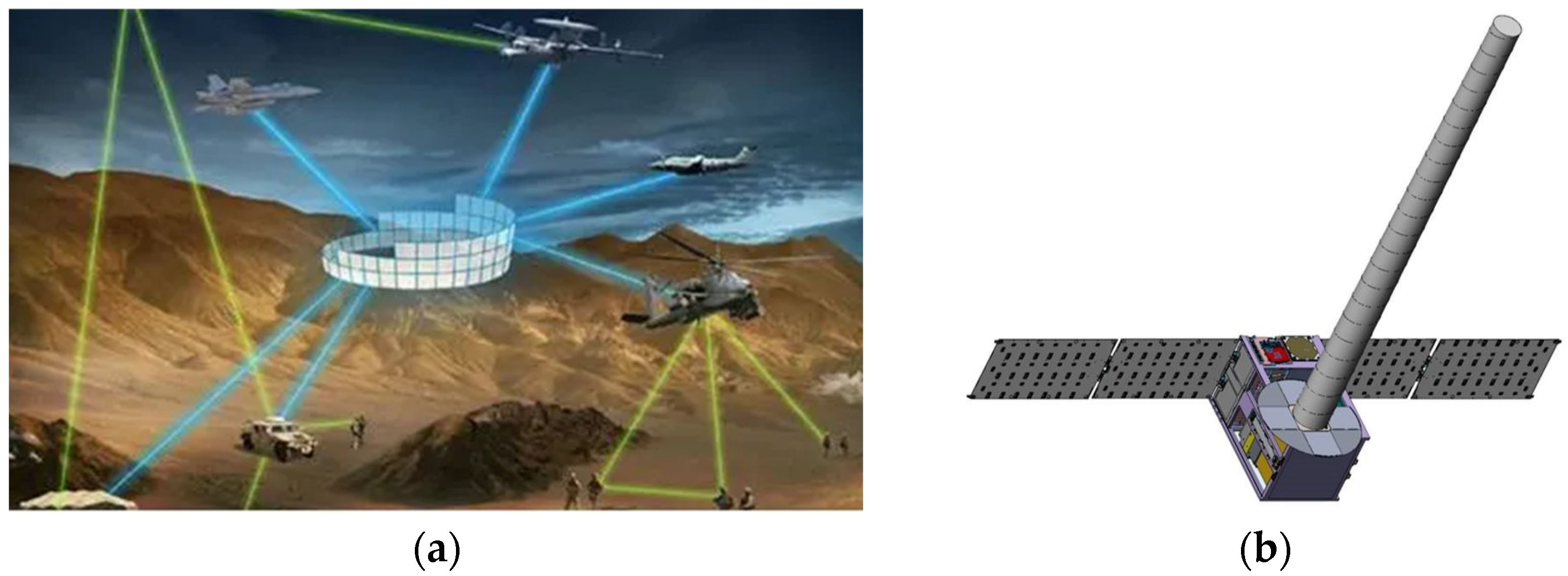
• This present manuscript presents results validating the declared state-of-the-art benchmark with tests on orbit using experimental satellites depicted in Figure 1.
• A seminal method is proposed and tested, and results are presented relative to the comparative benchmark.
• An additional novelty stems from the seminal introduction of a two-norm optimal projection learning method.

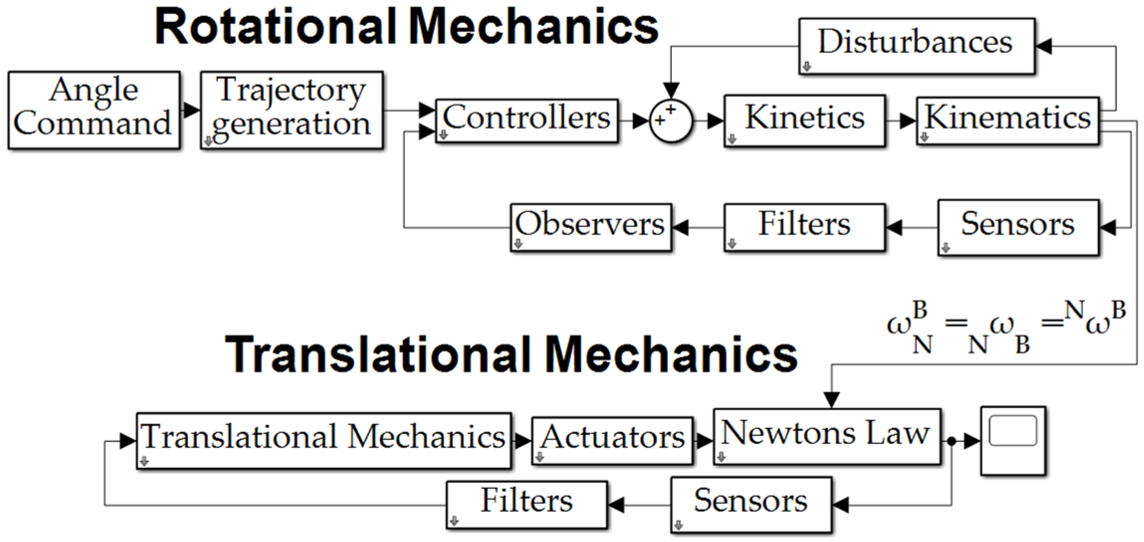
2. Materials and Methods

The methods adopted for this study accept a commonplace practice (displayed in Equation (1)) of analysis followed by the verification of analysis with modeling, simulation, and experimental validation using on-orbit space tests.

$$\begin{array}{ccccc}\boxed{Predict}& \to & \boxed{Test}& \to & \boxed{Validation}\end{array}$$

(1)

Analysis begins by defining the inertia matrix and components, while the mass center location is parameterized using the parallel axis theorem. Next, three estimation techniques are introduced as follows: a classical approach, nonlinear adaptive estimation (chosen as the comparative benchmark for this study), and two-norm optimal projection learning. The equations introduced in Section 2 are simulated in MATLAB^®/SIMULINK^®, R2022b and the simulation is briefly introduced, focusing on the overall simulation topology and the systems used to estimate the mass center location.

Periodically, short tables are presented to define proximal variables, acronyms, and such (e.g., Table 1, Table 2, Table 3, Table 4 and Table 5 and

Table A1. Table of proximal variables and nomenclature ¹.

Variable/Acronym	Definition
$H_{cm}$	Centroidal angular momentum
${\mathit{r}}_{dm,i}$	Radius vector to differential mass, $i$
$m_i$	Differential mass, $i$
$\mathit{\omega }$	Angular velocity vector
$\left\{\omega \right\}\equiv {\left\{\begin{array}{ccc}{\omega }_x& {\omega }_y& {\omega }_z\end{array}\right\}}^T$	Angular velocity [radians/second]
${\widehat{x}}_B,{\widehat{y}}_B,{\widehat{z}}_B$	Unit vectors
$x,y,z$	Positional coordinates
$J_y=J_O$	Inertia moment about a fixed axis $O$ along $y$
$J_{cm}$	Inertia moment about the mass center
$M$	Total system mass
$R_O$	Distance from O to the mass center
$R_y$	Distance to axis $y$
$O$	Fixed axis along axis $y$
$A,B,C$	Dummy variables
${\mathit{r}}_i$	Radius vector to point $i$
$dm$	Differential mass
${\mathit{v}}_{dm,i}$	Velocity vector of differential mass, $i$
$J_{xx},J_{yy},J_{zz}$	Moments of inertia
$J_{xy},J_{yx},J_{yz},J_{zy},J_{xz},J_{zx}$	Products of inertia
[$J$]	Moment of inertia matrix
$y$	Robot arm base parallel axis
$\widehat{y}$	Body center parallel axis
$r_{iO}$	Radius from parallel axis (not mass center)
$r_i$	Radius vector to the mass center
$m_i$	Differential mass element
($x_i,y_i)$	Center of mass coordinates
$a$	$x$ coordinate of $O$
$b$	$y$ coordinate of $O$
$\left[{\theta }_d\right]$	Desired angular state vector
$\left[{\omega }_d\right]$	Desired angular velocity vector
$\left[{\displaystyle \frac{d}{dt}}\left({\omega }_d\right)\right]$	Desired angular acceleration vector
$u_{fb}$	Feedback control
$K_p$	Proportional gain
$\left[\theta \right]$	Angular state vector
$\left[\omega \right]$	Angular velocity vector
$\left[{\displaystyle \frac{d}{dt}}\left(\omega \right)\right]$	Angular acceleration vector
$K_i$	Integral gain
$K_d$	Derivative gain

¹ Such tables are offered throughout the manuscript to aid readability.

) with a large summary table provided in Appendix B.

2.1. Inertia Matrix

Inertia matrices are ubiquitously diagonalized by transformation to the refence frame defined by the eigenvectors’ basis, eliminating the commonplace utility of off-diagonal inertia products. Accordingly, a very common derivation of all the terms of inertia matrices is presented next, especially due to the high importance of off-diagonal inertia products (remaining expressed in the body-fixed reference frame). The rigid body moments of inertia are defined in Equation (2) and expressed for the continuums of mass distributions in Equation (3). The vector identity in Equation (3) is used to modify Equation (3) into Equation (4), which simplifies to Equation (7)’s expression of the angular momentum vector. Defining the moment of inertia components in Equation (8) permits redefining the angular momentum terms, as displayed in Equation (9) formulated in matrix–vector form in Equation (10).

Table 1. Table of proximal variables and nomenclature ¹.

Variable/Acronym	Definition	Variable/Acronym	Definition
$H_{cm}$	Centroidal angular momentum	$A,B,C$	Dummy variables
${\mathit{r}}_{dm,i}$	Radius vector to differential mass, $i$	${\mathit{r}}_i$	Radius vector to point $i$
$m_i$	Differential mass, $i$	$dm$	Differential mass
$\mathit{\omega }$	Angular velocity vector	${\mathit{v}}_{dm,i}$	Velocity vector of differential mass, $i$

¹ Such tables are offered throughout the manuscript to aid readability.

Table 1. Table of proximal variables and nomenclature ¹.

Variable/Acronym	Definition	Variable/Acronym	Definition
$H_{cm}$	Centroidal angular momentum	$A,B,C$	Dummy variables
${\mathit{r}}_{dm,i}$	Radius vector to differential mass, $i$	${\mathit{r}}_i$	Radius vector to point $i$
$m_i$	Differential mass, $i$	$dm$	Differential mass
$\mathit{\omega }$	Angular velocity vector	${\mathit{v}}_{dm,i}$	Velocity vector of differential mass, $i$

¹ Such tables are offered throughout the manuscript to aid readability.

$$H_{cm}=\sum _{i=1}^n{\mathit{r}}_{dm,i}\times \underset{linear momentum}{\underbrace{m_i\left({\mathit{\omega }\times \mathit{r}}_{dm,i}\right)}}$$

(2)

$$H_{cm}=\underset{M}{\int }{\mathit{r}}_{dm,i}\times \underset{P=mv}{\underbrace{{\mathit{v}}_{dm,i}dm}}=\underset{M}{\int }{\mathit{r}}_{dm,i}\times \left({\mathit{\omega }\times \mathit{r}}_{dm,i}\right)dm$$

(3)

$$\mathrm{Use} \mathrm{vector} \mathrm{identity}: A\times B\times C=\left(A·C\right)B-\left(A·B\right)C$$

(4)

$$H_{cm}={\int }_M\left({\mathit{r}}_i·{\mathit{r}}_i\right)\mathit{\omega }-\left({\mathit{r}}_i·\mathit{\omega }\right){\mathit{r}}_{i}dm$$

(5)

$$\left({\mathit{r}}_i·\mathit{\omega }\right)\ne 0 \mathrm{u}\mathrm{n}\mathrm{l}\mathrm{e}\mathrm{s}\mathrm{s} \mathrm{p}\mathrm{l}\mathrm{a}\mathrm{n}\mathrm{a}\mathrm{r} \mathrm{b}\mathrm{o}\mathrm{d}\mathrm{y} \mathrm{w}\mathrm{i}\mathrm{t}\mathrm{h} 2\mathrm{D} \mathrm{m}\mathrm{o}\mathrm{t}\mathrm{i}\mathrm{o}\mathrm{n} \mathrm{i}\mathrm{n} \mathrm{i}\mathrm{t}\mathrm{s} \mathrm{o}\mathrm{w}\mathrm{n} \mathrm{p}\mathrm{l}\mathrm{a}\mathrm{n}\mathrm{e}$$

(6)

$$H_{cm}=\begin{array}{c}\left({\omega }_x\underset{M}{\int }\left(x^2+y^2+z^2\right)dm-\underset{M}{\int }\left({\omega }_{x}x+{\omega }_{y}y+{\omega }_{z}z\right)xdm\right){\widehat{x}}_B\\ +\left({\omega }_y\underset{M}{\int }\left(x^2+y^2+z^2\right)dm-\underset{M}{\int }\left({\omega }_{x}x+{\omega }_{y}y+{\omega }_{z}z\right)ydm\right){\widehat{y}}_B\\ +\left({\omega }_z\underset{M}{\int }\left(x^2+y^2+z^2\right)dm-\underset{M}{\int }\left({\omega }_{x}x+{\omega }_{y}y+{\omega }_{z}z\right)zdm\right){\widehat{z}}_B\end{array}$$

(7)

$$\begin{array}{cc}{J}_{xx}\equiv \underset{M}{\int }\left(y^2+z^2\right)dm,& J_{xy}=J_{yx}\equiv \underset{M}{\int }xydm\\ J_{yy}\equiv \underset{M}{\int }\left(x^2+z^2\right)dm,& J_{yz}=J_{zy}\equiv \underset{M}{\int }yzdm\\ J_{zz}\equiv \underset{M}{\int }\left(x^2+y^2\right)dm,& J_{xz}=J_{zx}\equiv \underset{M}{\int }xzdm\end{array}$$

(8)

$$H_{cm}=\begin{array}{c}\left(J_{xx}{\omega }_x-J_{xy}{\omega }_y-J_{xz}{\omega }_z\right){\widehat{x}}_B\\ +\left({-J}_{yx}{\omega }_x+J_{yy}{\omega }_y-J_{yz}{\omega }_z\right){\widehat{y}}_B\\ +\left(-J_{zx}{\omega }_x-J_{zy}{\omega }_y+J_{zz}{\omega }_z\right){\widehat{z}}_B\end{array}$$

(9)

$$\left\{H_{cm}\right\}=\underset{\left[J\right]}{\underbrace{\left[\begin{array}{ccc}{J}_{xx}& -J_{xy}& -J_{xz}\\ {-J}_{yx}& J_{yy}& -J_{yz}\\ -J_{zx}& -J_{zy}& J_{zz}\end{array}\right]}}\underset{\left\{\omega \right\}}{\underbrace{\left\{\begin{array}{c}{\omega }_x\\ {\omega }_y\\ {\omega }_z\end{array}\right\}}}$$

(10)

Table 2. Table of proximal variables and nomenclature ¹.

Variable/Acronym	Definition	Variable/Acronym	Definition
$\left\{\omega \right\}\equiv {\left\{\begin{array}{ccc}{\omega }_x& {\omega }_y& {\omega }_z\end{array}\right\}}^T$	Angular velocity [radians/second]	$J_{xx},J_{yy},J_{zz}$	Moments of inertia
${\widehat{x}}_B,{\widehat{y}}_B,{\widehat{z}}_B$	Unit vectors	$J_{xy},J_{yx},J_{yz},J_{zy},J_{xz},J_{zx}$	Products of inertia
$x,y,z$	Positional coordinates	$\left[J\right]$	Moment of inertia matrix

¹ Such tables are offered throughout the manuscript to aid readability.

Table 2. Table of proximal variables and nomenclature ¹.

Variable/Acronym	Definition	Variable/Acronym	Definition
$\left\{\omega \right\}\equiv {\left\{\begin{array}{ccc}{\omega }_x& {\omega }_y& {\omega }_z\end{array}\right\}}^T$	Angular velocity [radians/second]	$J_{xx},J_{yy},J_{zz}$	Moments of inertia
${\widehat{x}}_B,{\widehat{y}}_B,{\widehat{z}}_B$	Unit vectors	$J_{xy},J_{yx},J_{yz},J_{zy},J_{xz},J_{zx}$	Products of inertia
$x,y,z$	Positional coordinates	$\left[J\right]$	Moment of inertia matrix

¹ Such tables are offered throughout the manuscript to aid readability.

The derivation embodied in Equations (2)–(10) reveals time-varying mass distribution, where ${\mathit{r}}_{dm,i}={\mathit{r}\left(t\right)}_{dm,i}; m_i=m_i\left(t\right); \mathit{\omega }=\mathit{\omega }\left(\mathit{t}\right);$ and, similarly, the coordinates of differential masses: $x=x\left(t\right);y=y\left(t\right);z=z\left(t\right)$. Utilizing the time-varying nature necessitates some parameterization of the location of the mass center and some method of discerning the time-varying values of the inertia matrix. Next, in Section 2.2, the center of mass location is parameterized by assuming that the actual location is potentially (likely) unknown and not at the center of the body coordinate system. The parallel axis theorem is used to solve the three-dimensional coordinates of the mass center location. Afterwards, Section 2.3 introduces one option for inertia matrix component estimation.

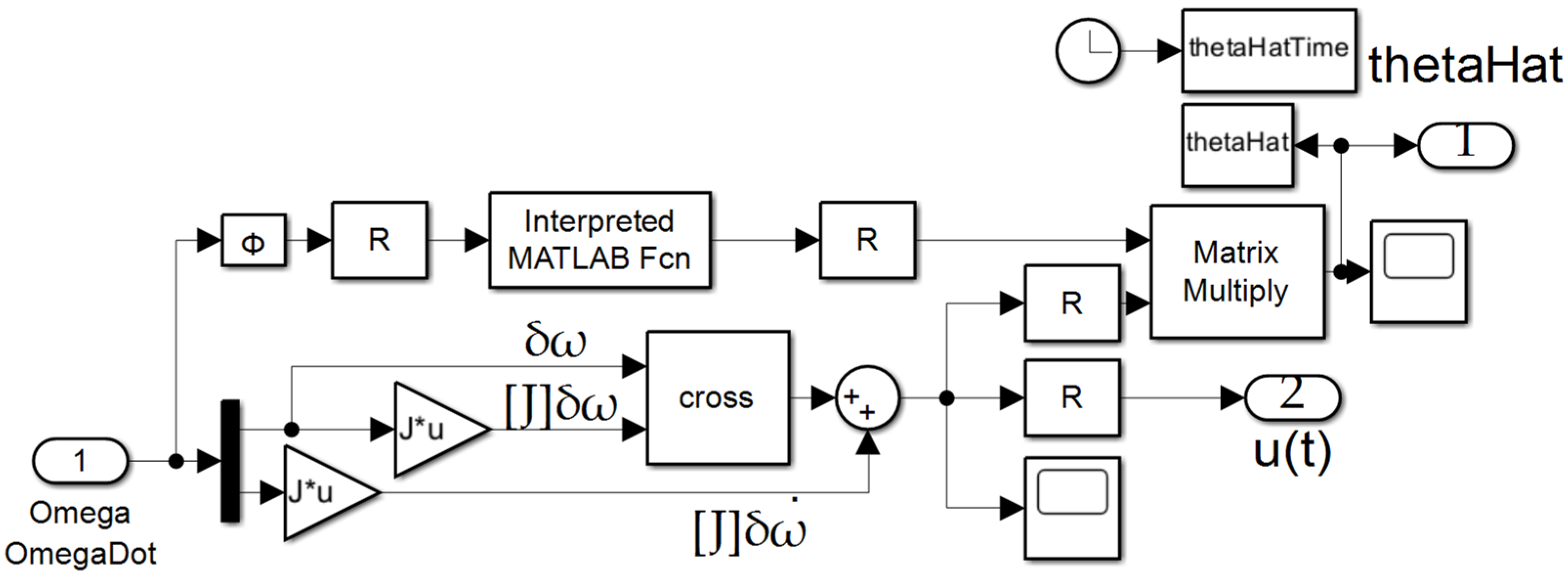
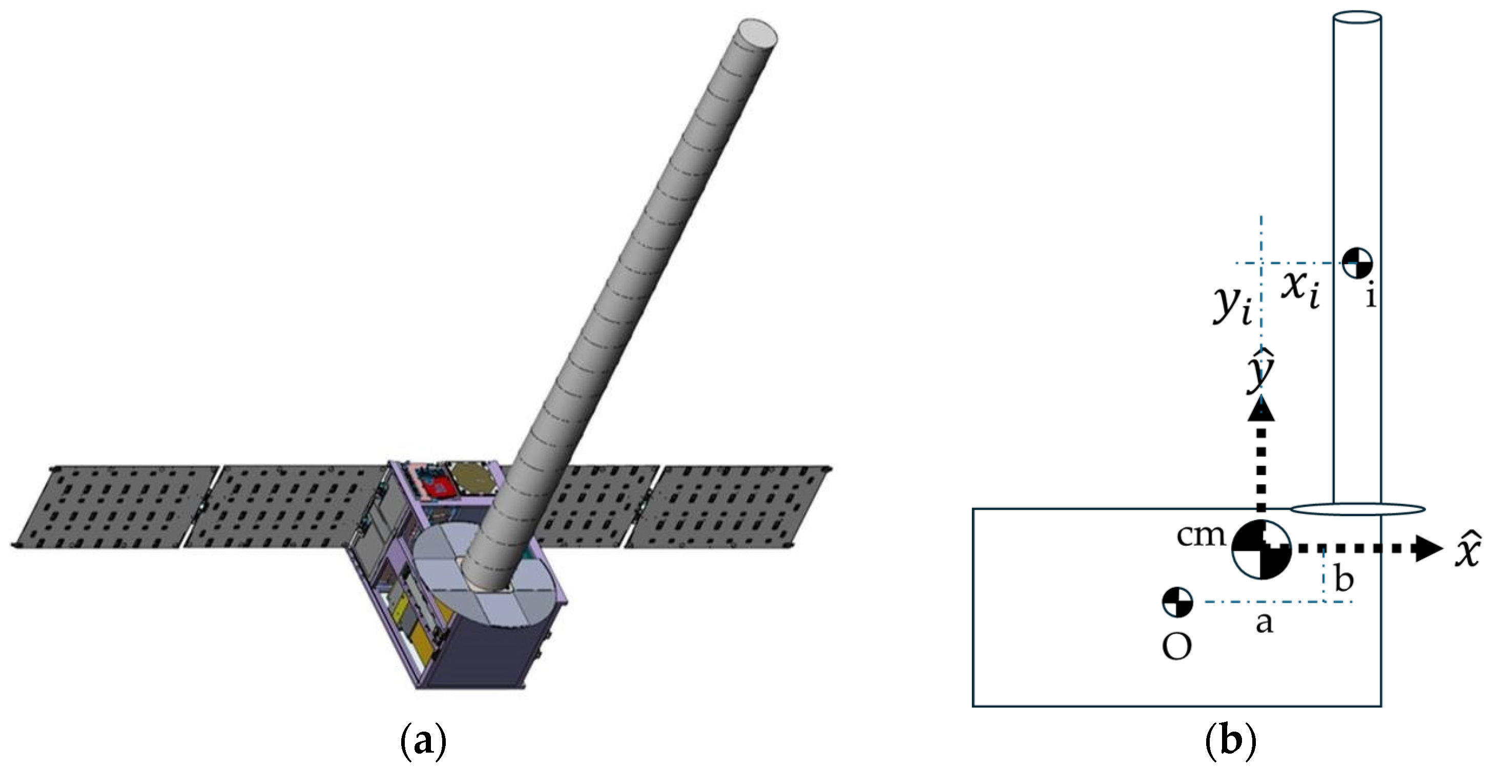
2.2. Center of Mass Location Estimation

By not diagonalizing the inertia matrix, off-balance rotation manifests in non-zero inertia products. Assuming the center of mass resides at some point other than the origin of the body-fixed axes, the parallel axis theorem (depicted in Figure 4) may be used to parameterize the location. Using such parameterization, the problem of estimating the location of the center of mass devolves into a commonplace problem of estimating the components of the inertia matrix, e.g., [30].

Theorem 1.

Parallel axis theorem. The moment of inertia  $J_O$ about some point other than the center of mass is the sum of the moment of inertia  $J_{cm}$ about the center of mass and the moment of inertia relative to the fixed distance between axes in the rigid body represented by the product of the total mass and the square of the distance (see Equation (11)).

$$J_O=J_{cm}+M{R}_O^2$$

(11)

The following proof mirrors [31], since the version most closely illuminates the use of the parallel axis theorem in this manuscript to reveal the three-dimensional location of the center of mass.

Proof. 

Consider a rigid system of particles of mass $M=\sum _i{m}_i$, rotating about a fixed axis $O$ along axis $y$. Place the origin of the coordinate system at the center-of-mass (cm) of our system of particles. The general point $i$ has coordinates ($x_i$, $y_i$), the $x$ coordinate of $O$ is a, and the $y$ coordinate of $O$ is $b$. Since the center of mass is at $\left(\mathrm{0,0}\right)$, by the definition of the center-of-mass (the unique point at any given time where the weighted relative position of the distributed mass sums to zero), Equation (12) results as follows:

Box 1. Key relationship between mass center location and inertia cross products.

$$\begin{array}{|ccc|}\hline x_{cm}=\sqrt{{\displaystyle \frac{J_{xy}{J}_{xz}}{m{J}_{yz}}}}& y_{cm}=\sqrt{{\displaystyle \frac{J_{xy}{J}_{yz}}{m{J}_{xz}}}},& z_{cm}=\sqrt{{\displaystyle \frac{J_{xz}{J}_{yz}}{m{J}_{xy}}}}\\ \hline\end{array}$$

(12)

□

By definition, $J_O=\sum _i{m}_i{r}_{iO}^2$, where $r_{iO}$ is measured from $O$, not from the mass center. Thus, $r_{iO}^2={\left(x_i-a\right)}^2+{\left(y_i-b\right)}^2$, leading to Equation (13). But, since $x_{cm}=\sum _i{\displaystyle \frac{m_i{x}_i}{M}}=0$ and similarly for $y$, the cross terms in Equation (13) go to zero once the sum over $i$ is finished, leading to Equation (14). Since $\left({x_i}^2+{y_i}^2\right)={r_i}^2$, where $r_i$ is now measured from the mass center, and $\left(a^2+b^2\right)={R_O}^2$ is just ${R_O}^2$, where $R_O$ is the distance from O to the mass center, Equations (13)–(15) result, whose terms are conveniently defined in Table 3.

$$J_O=\sum _i{m}_i\left[{\left(x_i-a\right)}^2+{\left(y_i-b\right)}^2\right]=\sum _i{m}_i\left[x_i^2-2a{x}_i+a^2+y_i^2-2b{y}_i^2+b^2\right]$$

(13)

$$J_O=\sum _i{m}_i\left({x_i}^2+{y_i}^2\right)+\sum _i{m}_i\left(a^2+b^2\right)$$

(14)

$$J_y=J_{cm}+M{R}_y^2$$

(15)

Table 3. Table of proximal variables and nomenclature ¹.

Variable/Acronym	Definition	Variable/Acronym	Definition
$J_y=J_O$	Inertia moment about a fixed axis $O$ along $y$	$y$	Robot arm base parallel axis
$J_{cm}$	Inertia moment about mass center	$\widehat{y}$	Body center parallel axis
$M$	Total system mass	$r_{iO}$	Radius from parallel axis (not mass center)
$R_O$	Distance from O to the mass center	$r_i$	Radius vector to the mass center
$R_y$	Distance to axis $y$	$m_i$	Differential mass element
$O$	Fixed axis along axis $y$	($x_i,y_i$)	Center of mass coordinates
$a$	$x$ coordinate of $O$	$b$	$y$ coordinate of $O$

¹ Such tables are offered throughout the manuscript to aid readability.

Table 3. Table of proximal variables and nomenclature ¹.

Variable/Acronym	Definition	Variable/Acronym	Definition
$J_y=J_O$	Inertia moment about a fixed axis $O$ along $y$	$y$	Robot arm base parallel axis
$J_{cm}$	Inertia moment about mass center	$\widehat{y}$	Body center parallel axis
$M$	Total system mass	$r_{iO}$	Radius from parallel axis (not mass center)
$R_O$	Distance from O to the mass center	$r_i$	Radius vector to the mass center
$R_y$	Distance to axis $y$	$m_i$	Differential mass element
$O$	Fixed axis along axis $y$	($x_i,y_i$)	Center of mass coordinates
$a$	$x$ coordinate of $O$	$b$	$y$ coordinate of $O$

¹ Such tables are offered throughout the manuscript to aid readability.

Having articulated the equations used to locate the mass center, the original problem has reduced to a different problem of inertia component identification. Next, in Section 2.3, the new problem solution is introduced by three disparate methods. The classical approach would necessitate estimating only the inertia moments (not products). The benchmark and proposed approaches estimate both moments and products, where only the products are used to analytically calculate the mass center location using Equation (12).

2.3. Inertia Matrix Component Estimation

One classical approach uses linearized double-integrator versions of the governing differential equations, while the benchmark for this study uses the full, coupled, and nonlinear equations with a simplified linear estimation. Meanwhile, the approach proposed also uses the full, coupled, and nonlinear equations with two-norm optimal projection learning.

2.3.1. Classical Approach

One ubiquitous classical approach displayed in Equation (16) is to treat the nonlinear coupled set of differential equations as if they were a simple uncoupled linear set of so-called double integrator equations. One necessary assumption is to treat the body axes as if they were equivalent to the eigen axes, diagonalizing the inertia matrix by transforming it to coordinates of a disparate reference frame of measurement (the frame spanned by the eigen axes).

$$\tau =\left[J\right]\left\{\dot{\omega }\right\}\to \left\{\begin{array}{c}{\tau }_x\\ {\tau }_y\\ {\tau }_z\end{array}\right\}=\left[\begin{array}{ccc}{J}_x& 0& 0\\ 0& J_y& 0\\ 0& 0& J_z\end{array}\right]\left\{\begin{array}{c}{\dot{\omega }}_x\\ {\dot{\omega }}_y\\ {\dot{\omega }}_z\end{array}\right\}=\left\{\begin{array}{c}{J_x\dot{\omega }}_x\\ J_y{\dot{\omega }}_y\\ J_z{\dot{\omega }}_z\end{array}\right\}\to \left\{\begin{array}{c}{\tau }_x\\ {\tau }_y\\ {\tau }_z\end{array}\right\}=\left\{\begin{array}{c}{J_x\dot{\omega }}_x\\ J_y{\dot{\omega }}_y\\ J_z{\dot{\omega }}_z\end{array}\right\}$$

(16)

The approach is simple: divide the known torque components by the component angular velocity to reveal the principal moment (not product) of inertia for each of the three axes.

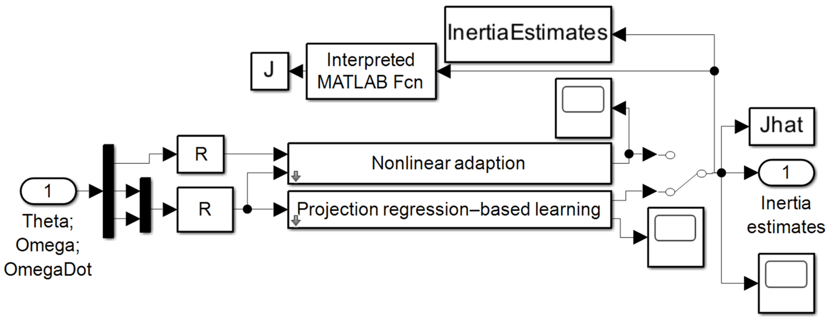
2.3.2. Comparative Benchmark Approach (Nonlinear Adaptive Estimation)

The comparative benchmark approach for this study parameterizes the nonlinear coupled set of differential equations into a system matrix, $\mathsf{\Phi }$, with the inertia matrix components used to form the regression vector, $\beta$, where this parameterization is adopted in the proposed approach described in Section 2.3.3. The rate of change of the regression vector is defined in negative feedback with a combined measure of trajectory tracking error, $\mathit{s}$, using a positive constant, $\mathsf{\Gamma }$, as the adaption gain displayed in Equations (17) and (18).

$$\dot{\widehat{\beta }}=-{\mathsf{\Gamma }}^{-1}{\mathsf{\Phi }}^T\mathit{s}$$

(17)

$$\mathit{s}=\ddot{\theta }+\lambda \dot{\theta }$$

(18)

2.3.3. Proposed Approach (Two-Norm Optimal Projection Learning)

Identical regression parameterization (displayed in Equation (20)) is maintained in the proposed approach, where the feedback-based gain adaption is replaced with projection learning based on two-norm optimal least squares, as indicated in Equation (21), where terms are conveniently defined in Table 4.

$$\tau =\left[J\right]\left\{\dot{\omega }\right\}+\left\{\omega \right\}\times \left[J\right]\left\{\omega \right\}$$

(19)

$$\tau =\underset{{\left[\mathsf{\Phi }\right]}_d}{\underbrace{{\underbrace{\left[\begin{array}{cccccc}{\dot{\omega }}_x& {\dot{\omega }}_y-{\omega }_x{\omega }_z& {\dot{\omega }}_z-{\omega }_x{\omega }_y& -{\omega }_y{\omega }_z& 0& {\omega }_y{\omega }_z\\ {\omega }_x{\omega }_z& {\dot{\omega }}_x+{\omega }_y{\omega }_z& 0& {\dot{\omega }}_y& {\dot{\omega }}_z-{\omega }_x{\omega }_y& -{\omega }_x{\omega }_z\\ -{\omega }_x{\omega }_y& 0& {\dot{\omega }}_x-{\omega }_y{\omega }_z& {\omega }_x{\omega }_y& {\dot{\omega }}_y+{\omega }_x{\omega }_z& {\dot{\omega }}_z\end{array}\right]}}_d}}\underset{\widehat{\beta }}{\underbrace{\left\{\begin{array}{c}{\widehat{J}}_{xx}\\ {\widehat{J}}_{xy}\\ {\widehat{J}}_{xz}\\ {\widehat{J}}_{yy}\\ {\widehat{J}}_{yz}\\ {\widehat{J}}_{zz}\end{array}\right\}}}$$

(20)

$$\widehat{\beta }={\left\{\begin{array}{cccccc}{\widehat{J}}_{xx}& {\widehat{J}}_{xy}& {\widehat{J}}_{xz}& {\widehat{J}}_{yy}& {\widehat{J}}_{yz}& {\widehat{J}}_{zz}\end{array}\right\}}^T={\left[\Phi \right]}_d{\left({{\left[\Phi \right]}_d}^T{\left[\Phi \right]}_d\right)}^{-1}{\left[\Phi \right]}_d\tau$$

(21)

Table 4. Table of proximal variables and nomenclature ¹.

Variable/Acronym	Definition	Variable/Acronym	Definition
${\left[{\omega }_x\right]}_d$	Desire angular velocity about $\widehat{x}$	${\left[{\dot{\omega }}_x\right]}_d$	Desire angular acceleration about $\widehat{x}$
${\left[{\omega }_y\right]}_d$	Desire angular velocity about $\widehat{y}$	${\left[{\dot{\omega }}_y\right]}_d$	Desire angular acceleration about $\widehat{y}$
${\left[{\omega }_z\right]}_d$	Desire angular velocity about $\widehat{z}$	${\left[{\dot{\omega }}_z\right]}_d$	Desire angular acceleration about $\widehat{z}$
$\left[\Phi \right]=\Phi$	Regression matrix of sensor data	${\left[\Phi \right]}_d={\Phi }_d$	Regression matrix of desired states
$\beta$	Unknown predicted variables	$\widehat{\beta }$	Estimated variables
$\tau$	Total control torque signal	${\tau }_{ff}$	Feedforward control signal
${\widehat{J}}_{xx}$	Estimated moment of inertia about $\widehat{x}$	${\widehat{J}}_{xy}={\widehat{J}}_{yx}$	Estimated $\widehat{x}\widehat{y}$ inertia product
${\widehat{J}}_{yy}$	Estimated moment of inertia about $\widehat{y}$	${\widehat{J}}_{xz}={\widehat{J}}_{zx}$	Estimated $\widehat{x}\widehat{z}$ inertia product
${\widehat{J}}_{zz}$	Estimated moment of inertia about $\widehat{z}$	${\widehat{J}}_{yz}={\widehat{J}}_{zy}$	Estimated $\widehat{y}\widehat{z}$ inertia product

¹ Such tables are offered throughout the manuscript to aid readability.

Table 4. Table of proximal variables and nomenclature ¹.

Variable/Acronym	Definition	Variable/Acronym	Definition
${\left[{\omega }_x\right]}_d$	Desire angular velocity about $\widehat{x}$	${\left[{\dot{\omega }}_x\right]}_d$	Desire angular acceleration about $\widehat{x}$
${\left[{\omega }_y\right]}_d$	Desire angular velocity about $\widehat{y}$	${\left[{\dot{\omega }}_y\right]}_d$	Desire angular acceleration about $\widehat{y}$
${\left[{\omega }_z\right]}_d$	Desire angular velocity about $\widehat{z}$	${\left[{\dot{\omega }}_z\right]}_d$	Desire angular acceleration about $\widehat{z}$
$\left[\Phi \right]=\Phi$	Regression matrix of sensor data	${\left[\Phi \right]}_d={\Phi }_d$	Regression matrix of desired states
$\beta$	Unknown predicted variables	$\widehat{\beta }$	Estimated variables
$\tau$	Total control torque signal	${\tau }_{ff}$	Feedforward control signal
${\widehat{J}}_{xx}$	Estimated moment of inertia about $\widehat{x}$	${\widehat{J}}_{xy}={\widehat{J}}_{yx}$	Estimated $\widehat{x}\widehat{y}$ inertia product
${\widehat{J}}_{yy}$	Estimated moment of inertia about $\widehat{y}$	${\widehat{J}}_{xz}={\widehat{J}}_{zx}$	Estimated $\widehat{x}\widehat{z}$ inertia product
${\widehat{J}}_{zz}$	Estimated moment of inertia about $\widehat{z}$	${\widehat{J}}_{yz}={\widehat{J}}_{zy}$	Estimated $\widehat{y}\widehat{z}$ inertia product

¹ Such tables are offered throughout the manuscript to aid readability.

$$\begin{array}{ccccc}\boxed{Analysis}& \to & \boxed{Simulation verification}& \to & \boxed{Experimental validation}\end{array}$$

(22)

As reminded by Equation (22), following the analysis, modeling and simulation preface experimental validating spaceflight tests. Figure 5 contains a top level topology of spacecraft guidance and control, where this study focuses exclusively on the rotational mechanics subsystems. This topology is provided by the very simulation used to verify the analysis. Within the subsystem labeled “Controllers”, novel subsystems are created to estimate and to learn the inertia components (displayed in Figure 6), while the mass center location is simulated in the attitude control system displayed in Figure 7, where nomenclature is conveniently defined in Table 5.

Table 5. Table of proximal variables and nomenclature ¹.

Variable/Acronym	Definition	Variable/Acronym	Definition
$\left[{\theta }_d\right]$	Desired angular state vector	$\left[\theta \right]$	Angular state vector
$\left[{\omega }_d\right]$	Desired angular velocity vector	$\left[\omega \right]$	Angular velocity vector
$\left[{\displaystyle \frac{d}{dt}}\left({\omega }_d\right)\right]$	Desired angular acceleration vector	$\left[{\displaystyle \frac{d}{dt}}\left(\omega \right)\right]$	Angular acceleration vector
$u_{fb}$	Feedback control	$K_i$	Integral gain
$K_p$	Proportional gain	$K_d$	Derivative gain

¹ Such tables are offered throughout the manuscript to aid readability.

Table 5. Table of proximal variables and nomenclature ¹.

Variable/Acronym	Definition	Variable/Acronym	Definition
$\left[{\theta }_d\right]$	Desired angular state vector	$\left[\theta \right]$	Angular state vector
$\left[{\omega }_d\right]$	Desired angular velocity vector	$\left[\omega \right]$	Angular velocity vector
$\left[{\displaystyle \frac{d}{dt}}\left({\omega }_d\right)\right]$	Desired angular acceleration vector	$\left[{\displaystyle \frac{d}{dt}}\left(\omega \right)\right]$	Angular acceleration vector
$u_{fb}$	Feedback control	$K_i$	Integral gain
$K_p$	Proportional gain	$K_d$	Derivative gain

¹ Such tables are offered throughout the manuscript to aid readability.

2.4. Implementation Procedure

Substantial modeling and simulations are performed and presented in references [29,30], where a very brief summary of key findings is presented in Section 3. The review of modeling and simulation results serves as a preface to the spaceflight experiments.

3. Results

This section presents the on-orbit experimental results after reviewing the key findings from modeling and simulation. The computational models that analyzed the data are depicted in Appendix A. Section 3.1 includes the key modeling and simulation results, while Section 3.2 includes the key results from spaceflight experiments, including mass inertia identification and center of mass auto-location. Figure 8 displays the spacecraft mounted in a rideshare stack on the launch vehicle and the 2023 launch to space.

3.1. Key Results from Modeling and Simulation

Estimated products of inertia are fed to Equation (12) to determine the location of the center of gravity (i.e., center of mass), where the inertia products may alternatively be estimated by nonlinear adaptive estimation (Equation (17)) or by two-norm optimal projection learning (Equation (21)), respectively, in Section 3.1.1 and Section 3.1.2. To aid repeatability, SIMULINK^® systems and subsystems, and MATLAB^® line code used in the SIMULINK^® callbacks are provided in this Appendix A.

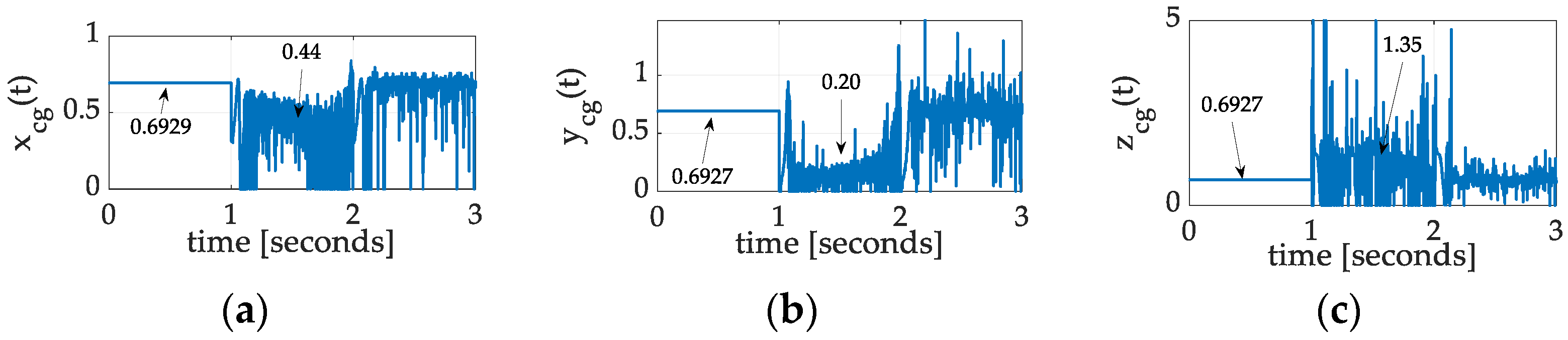
3.1.1. Center of Gravity Auto-Location by Nonlinear Adaption

Auto-location adaption is apparent twice in Figure 9 in response to the single axis rotational slew maneuver. The estimated location migrates roughly 0.15, 0.1 $\pm 0.02$, and 0.225 m, respectively, in the $\widehat{x}$, $\widehat{y}$, and $\widehat{z}$ directions, and then migration completely stops when the excitation of the maneuver ends. In particular, notice the location does not converge to an identifiable place during the maneuver, and the results may be deemed as unsuccessful.

3.1.2. Center of Gravity Auto-Location by Nonlinear Projection-Based Regression Learning

Auto-location adaption is apparent only once in Figure 10 in response to the single axis rotational slew maneuver. The estimated location converges to roughly 0.2529 m aft ($\widehat{x}$), 0.4927 m less in $\widehat{y}$, and 0.225 m up in $\widehat{z}$. Since the simulated mass center location is known, in particular, notice that the location converges to an identifiable place very quickly after maneuver initiation, and the results may be deemed successful.

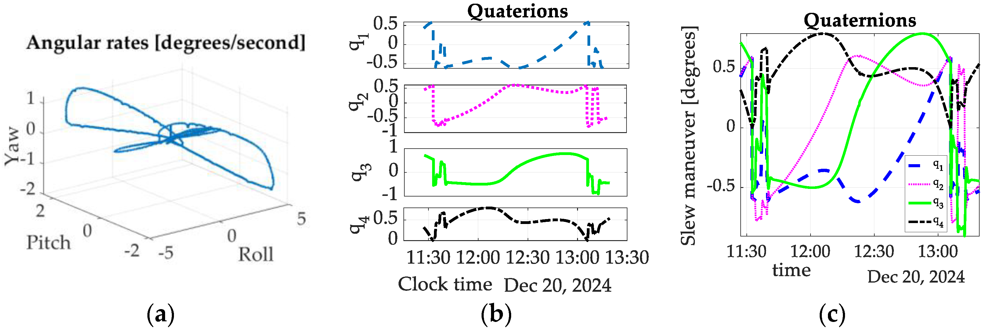
3.2. Key Results from Spaceflight Experiments Flown on 20 December 2024

Much like the recent validation of inertia identification in space studied by Nocerino, et al. [34], the methods presented here are similarly validating with spaceflight experiments flown in December of 2024. Key results are first presented with rate data from the onboard sensors during the spaceflight test. Next, wheel torques and quaternion (relative to an earth centered inertial coordinate system) data provided by the satellite operators are presented together with attitude angles produced by mathematical analysis of rate data, assuming a 3–2–1 rotation sequence. Such a sequence expresses the rotation angle as a yaw rotation about the inertial $\widehat{z}$ axis followed by a pitch rotation about an intermediate $\widehat{y}$ axis (between the inertial and body frames), and then, finally, a roll rotation about the body $\widehat{x}$ axis.

Figure 11a presents the angular rates and quaternions, while Figure 12 provides different displays of Euler angles.

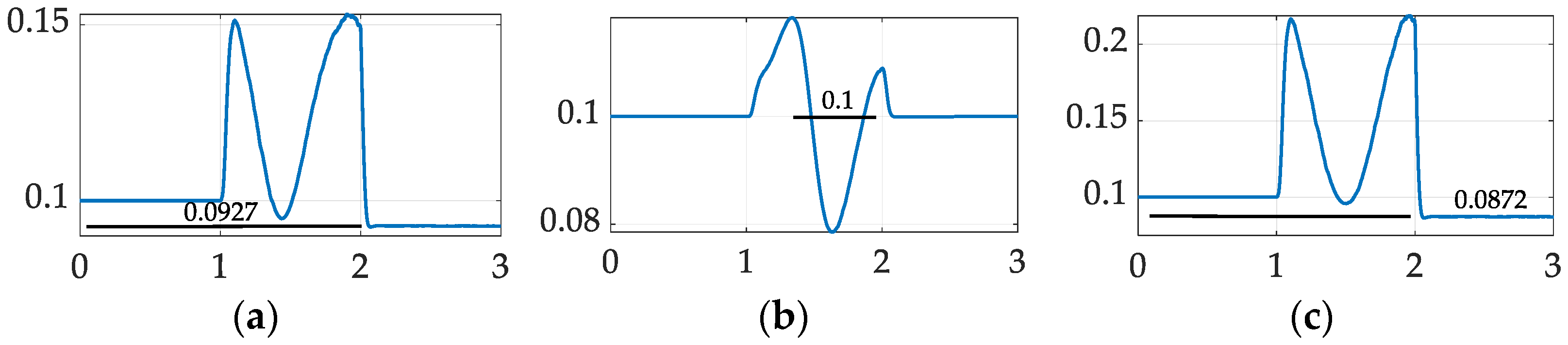
3.3. Inertia Auto-Identification

Figure 13 displays the roll, pitch, and yaw angle estimation errors achieved by the nonlinear enhanced Luenberger observers. The observers are chosen to leverage their rapid field-tunable nature. Notice the limited estimation accuracy achieved by the rapid field tuning of observer gains that might potentially limit the eventual convergence of the auto-location algorithm, which is elaborated in Section 3.4. Impacts on intermediate quantities (estimated mass moments and products of inertia) are seemingly only mildly affected, as displayed in Figure 14.

3.4. Center of Mass Location Auto-Location

Inertia estimation by nonlinear adaption and by nonlinear projection-based regression learning is calculated using Equation (17) and Equation (21), respectively. Using those estimates, the location of the center of mass is found by Equation (12). The location using nonlinear adaption is displayed in Figure 15, while the location using nonlinear projection-based regression learning is displayed in Figure 16.

As a reminder of the results of modeling and simulation from [29,30], Figure 15 illustrates the relative ineffectiveness of nonlinear adaption to auto-locate the center of gravity. The algorithm indeed quickly diverges from the initially estimated location; however, it does not consistently converge to a new (presumably correct) location. Instead, it oscillates inconsistently, which is a ubiquitous feature of nonlinear adaption, where parameters are adjusted based on the M.I.T. rule [35].

Figure 16 displays the results of space experiments flown 20 December 2024 using projection regression-based learning time-varying location of the center of mass. According to Figure 16a, the mass about the $\widehat{x}$ axis is seemingly well balanced. Meanwhile, the mass about the $\widehat{y}$ axis is quite off-balance according to Figure 16b, and the learned location converges to 34.80 cm. Similarly, the mass about the $\widehat{z}$ axis is quite off-balance according to Figure 16c, and the learned location converges to 34.39 cm. Two subsequent validating experiments are executed, and the converged values of mass center location are essentially identical to the initial experimental results.

4. Discussion

The study results confirmed the roll axis was probably well aligned, while the other two axes had erroneous mass and inertia distribution assumptions. The rapidly convergent mass center coordinates oscillated slightly before final convergence. The use of nonlinear enhanced Luenberger observers should be the source of such slight oscillations. The observers are classical control forms that ubiquitously induce oscillatory settling. The oscillations were most pronounced in the output of the observers (state estimates), relatively ameliorated in the subsequent inertia estimation, and even further ameliorated in the location estimates. The convergent inertia estimation indicates potential efficacy responding to grappling objects of unknown mass and inertia properties and possible mass gain and loss due to collisions in space.

The original problem statement described how inertia moments were proposed to be estimated in space during maneuvering operations rather than on the ground, while the estimation of inertia products would be performed using the introduced parameterization of the location of the mass center using the parallel axis theorem. Estimation of the time-varying inertia properties thereby leads to the auto-location of the spacecraft’s center of mass. The original research objectives were illustrated by using only empirical attitude angle knowledge to find imbalanced inertia components and then convert that mass imbalance to center of gravity coordinates. Auto-location of the center of gravity was seminally illustrated with estimation convergence improvements over the comparative state-of-the-art benchmark. Improvements achieved included great convergence that was also faster, i.e., from millimeter convergence over hundreds of days to hundreds of millimeters in minutes achieved in this study. Unexpectedly, relatively poor motion state estimation was used to nonetheless produce rapid accurate estimation of the location of the mass center.

Future Research Directions

Recommended future research is conveniently tabularized below, with sub-tabularized rationale, purpose served, and expected outcomes:

• Enhance Luenberger observer tuning for improved accuracy.
  • Rationale: Figure 13 reveals poor state estimation errors that nonetheless led to precise estimation of inertia components and mass center location. Very recent attempts to repeat these experiments produced similar results, but subsequent experiments on a different spacecraft (seeking generalizability) did not produce good inertia estimation or mass center location estimation. Since all other aspects of the proposed method are analytic, the remaining potential cause of the loss of estimation performance is the relatively poor state estimation.
  • Purpose served: continue to seek generalizable application to any spacecraft.
  • Expected outcomes: improved inertia estimation should lead to robust gravity center estimation.
• Empirical validation of these initial results.
  • Rationale: experimental validation of analytic and simulation results necessitate repeatability and generalizability.
  • Purpose served: expand the applicability of the proposed methods.
  • Expected outcomes: increased inertia estimation accuracy should improve the inputs to (12), directly leading to robust mass center location estimation.
• Grapple with objects of unknown mass.
  • Rationale: space robotic grappling requires rapid inertia identification and mass center location to update guidance and control systems.
  • Purpose served: improves stability and accuracy.
  • Expected outcomes: substantially improves robustness and accuracy.
• Recover from collision damage with significant mass losses and/or gains.
  • Rationale: spacecraft that have experienced such collisions need autonomous methods to rapidly update system models to recommence operations.
  • Purpose served: autonomously recovers from substantial damage.
  • Expected outcomes: Equation (20) retains utility for control with updated mass center and inertia components.
• Application of these methods to flexible spacecraft.
  • Rationale: flexible spacecraft modeling can be more realistic and typically follows rigid body treatments to ascertain whether the higher order modeling is necessary.
  • Purpose served: potentially increases modeling accuracy.
  • Expected outcomes: potential increase in grappling ability.
• Sensitivity analysis how angular velocity cross terms affect the conditioning of the regression matrix.
  • Rationale: to justify using the higher order model, including the transport theorem cross products, rather than the ubiquitous so-called double integrator model.
  • Purpose served: potentially ability to use simplified models without increasing model accuracy.
  • Expected outcomes: potential decrease in computational burden.

References

1. SDA Gets OK to Begin Limited Testing of Data Satellites Link 16 Nodes. Available online: https://www.sda.mil/sda-gets-ok-to-begin-limited-testing-of-data-satellites-link-16-nodes/ (accessed on 16 December 2024).
2. Department of Defense Photographs and Imagery, Unless Otherwise Noted, Are in the Public Domain. Use of Department of Defense Imagery. Available online: https://www.defense.gov/Contact/Help-Center/Article/Article/2762906/use-of-department-of-defense-imagery/ (accessed on 16 December 2024).
3. Nanosats Database: XVI Satellite. Available online: https://www.nanosats.eu/sat/xvi (accessed on 16 December 2024).
4. Available online: https://www.usna.edu/Users/aero/kang/Research.php#panel3RSatPRoboticArmSatellitePrototype (accessed on 4 February 2025).
5. Wei, X.; Huang, L.; Shen, T.; Cai, Z. Calibration of the in-orbit center-of-mass of TaiJi-1. arXiv 2024, arXiv:2307.01724v2. [Google Scholar] [CrossRef]
6. Otsubo, T.; Appleby, G. System-dependent center-of-mass correction for spherical geodetic satellites. J. Geophys. Res. 2003, 108, 2201. [Google Scholar] [CrossRef]
7. Rodríguez, J.; Appleby, G.; Otsubo, T. Upgraded modelling for the determination of centre of mass corrections of geodetic SLR satellites: Impact on key parameters of the terrestrial reference frame. J. Geod. 2019, 93, 2553–2568. [Google Scholar] [CrossRef]
8. Rodríguez, J. Centre of Mass Corrections Updates for Geodetic Spherical Satellites: Changes in the Latest Releases in Preparation for the Computation of ITRF2020 Products; Technical Report IT-CDT 2022-11; Yebes Observatory: Yebes, Spain, 22 November 2022. [Google Scholar]
9. Geosat: U.S. Navy GEOdetic SATellite. Available online: https://science.nasa.gov/mission/geosat/ (accessed on 16 December 2024).
10. NASA Images and Media Usage Guidelines. Available online: https://www.nasa.gov/nasa-brand-center/images-and-media/ (accessed on 16 December 2024).
11. Neubert, R. The Retro-Reflector for the CHAMP Satellite: Final Design and Realization. In Proceedings of the 11th International Laser Ranging Workshop, Deggendorf, Germany, 21–25 September 1988. [Google Scholar]
12. International Laser Ranging Service: Etalon-1 and -2: Array Offset Information. Available online: https://ilrs.gsfc.nasa.gov/missions/satellite_missions/current_missions/eta1_com.html (accessed on 16 December 2024).
13. International Laser Ranging Service: Galileo: Array Offset Information. Available online: https://ilrs.gsfc.nasa.gov/missions/satellite_missions/current_missions/ga01_com.html (accessed on 16 December 2024).
14. Lemoine, F.; Rowlands, D.; Lillibridge, J.; Smith, W.; Zelensky, N.; Beckley, B.; Chinn, D.; Scharroo, R. Evaluation of the GEOSAT and GEOSAT Follow-On Precise Orbit Ephemeris. In Proceedings of the 2007 Ocean Surface Topography Science Team Meeting, Hobart, Australia, 12–15 March 2007; Available online: https://www.aviso.altimetry.fr/fileadmin/documents/OSTST/2007/lemoine_gfo_pod.pdf (accessed on 16 December 2024).
15. Hernández-Arias, H.; Prado-Molina, J. On-Orbit Center Of Mass Relocation System For a 3U Cubesat. Int. J. Sci. Technol. Res. 2018, 7, 44–51. [Google Scholar]
16. Alharam, A.; Albalooshi, A.; Sleptchenko, A. Linear cubesat center of gravity optimization. In Proceedings of the AerospaceEurop Confrence 2021, Warsaw, Poland, 23–26 November 2021. [Google Scholar]
17. Al-Rawashdeh, Y.M.; Elshafei, M.; Al-Malki, M.F. In-Flight Estimation of Center of Gravity Position Using All-Accelerometers. Sensors 2014, 14, 17567–17585. [Google Scholar] [CrossRef] [PubMed]
18. Zhao, X.; Xiao, W. Uncertainty Analysis of Aircraft Center of Gravity Deviation and Passenger Seat Allocation Optimization. Mathematics 2024, 12, 1591. [Google Scholar] [CrossRef]
19. Wu, F.; Sun, C.; Li, H.; Zheng, S. Real-Time Center of Gravity Estimation for Intelligent Connected Vehicle Based on HEKF-EKF. Electronics 2023, 12, 386. [Google Scholar] [CrossRef]
20. Park, G.; Choi, S.B. An Integrated Observer for Real-Time Estimation of Vehicle Center of Gravity Height. IEEE Trans. Intell. Transp. Syst. 2021, 22, 5660–5671. [Google Scholar] [CrossRef]
21. Huang, X.; Wang, J. Real-Time Estimation of Center of Gravity Position for Lightweight Vehicles Using Combined AKF–EKF Method. IEEE Trans. Veh. Technol. 2014, 63, 4221–4231. [Google Scholar] [CrossRef]
22. Lin, C.; Gong, X.; Xiong, R.; Cheng, X. A novel H∞ and EKF joint estimation method for determining the center of gravity position of electric vehicles. Appl. Energy 2017, 194, 609–616. [Google Scholar] [CrossRef]
23. Fu, Z.; Hu, Q.; Li, B. Adaptive online estimation of centre of gravity height for commercial vehicles. Int. J. Heavy Veh. Syst. 2021, 28, 206–225. [Google Scholar] [CrossRef]
24. Han, X.; Li, Z.; Li, H.; Huang, L.; Pang, Y. Variable mass control and parameter identification of spacecraft orbit refueling process. Math. Prob. Eng. 2022, 17, 9660218. [Google Scholar] [CrossRef]
25. Gaine Technology. Probabilistic and Deterministic Results in AI Systems. 31 July 2023. Available online: https://www.gaine.com/blog/probabilistic-and-deterministic-results-in-ai-systems (accessed on 11 March 2024).
26. Holubek, R.; Vagaš, M. Center of Gravity Coordinates Estimation Based on an Overall Brightness Average Determined from the 3D Vision System. Appl. Sci. 2022, 12, 286. [Google Scholar] [CrossRef]
27. Moulton, B.C.; Hunsaker, D.F. Analytic Solutions for Volume, Mass, Center of Gravity, and Inertia of Wing Segments and Rotors of Constant Density. Aerospace 2024, 11, 492. [Google Scholar] [CrossRef]
28. Liu, F.; Su, Z.; Zhao, H.; Li, Q.; Li, C. Attitude Measurement for High-Spinning Projectile with a Hollow MEMS IMU Consisting of Multiple Accelerometers and Gyros. Sensors 2019, 19, 1799. [Google Scholar] [CrossRef] [PubMed]
29. Sands, T.; Kim, J.J.; Agrawal, B.N. Spacecraft fine tracking pointing using adaptive control. In Proceedings of the 58th International Astronautical Congress, Hyderabad, India, 24–28 September 2007. [Google Scholar]
30. Sands, T. Autonomous Real–Time Mass Center Location and Inertia Identification for Grappling Space Robotics. Technologies 2025, 13, 148. [Google Scholar] [CrossRef]
31. Adams, G. Arizona State University Physics Department Proof of the Parallel Axis Theorem. Available online: https://www.public.asu.edu/~gbadams/sum00/parallelaxisT.pdf (accessed on 16 December 2024).
32. SatCatalog. Available online: https://www.satcatalog.com/component/rwp050/ (accessed on 16 December 2024).
33. Foust, J. SpaceX Launches Eighth Dedicated Smallsat Rideshare Mission. Available online: https://spacenews.com/spacex-launches-eighth-dedicated-smallsat-rideshare-mission/ (accessed on 11 March 2025).
34. Alessia Nocerino, A.; Opromolla, R.; Fasano, G.; Grassi, M.; Balaguer, P.; John, S.; Cho, H.; Bevilacqua, R. Experimental validation of inertia parameters and attitude estimation of uncooperative space targets using solid state LIDAR. Acta Astronaut. 2023, 210, 428–436. [Google Scholar] [CrossRef]
35. Gupta, D.; Kumar, A.; Giri, V. Effect of adaptation gain and reference model in MIT and Lyapunov rule–based model reference adaptive control for first- and second-order systems. Trans. Inst. Meas. Control 2024, 46, 1635–1654. [Google Scholar] [CrossRef]
Figure 2. U.S. Naval cubesat grappling space robot (images credit: U.S. Navy), launched in 2018 [4]. Used in accordance with published image use policy [2]. (a) Computer-aided drawing depicting two robotic arms with cameras on each end effector and at the cube satellite’s mid-body; (b) actual hardware with robot arms stowed.
Technologies 13 00246 g002
Figure 3. (a) Center of mass correction concept from [7,8] for satellites with laser retroreflector arrays (LRA). (b) U.S. Navy GEOSAT spacecraft [9]. Image credit: NASA. Used in accordance with image use policy [10].
Technologies 13 00246 g003
Figure 4. (a) Air Force Research Laboratory (AFRL) XVI satellite, host of Link 16 payload. [3] (b) Schematic of center of mass offset from spacecraft body axes centered at origin, O, corresponding to the parallel axis theorem.
Technologies 13 00246 g004
Figure 5. Top level topology of spacecraft guidance and control. More detailed elaboration of modeling and simulation may be found in [29,30].
Technologies 13 00246 g005
Figure 6. Inertia matrix component identification schemes. (a) Learning feedback inertia matrix estimator elaborated in Equation (21) [32]; (b) nonlinear adaptive inertia estimation scheme in accordance with Equation (17).
Technologies 13 00246 g006
Figure 7. Attitude determination and control system simulated in MATLAB®/SIMULINK®.
Technologies 13 00246 g007
Figure 8. Source of known torques τ x τ y τ z T in Equation (16); onboard set of three reaction wheels. (a) XVI (depicted in Figure 1 and Figure 3) spacecraft stacked in a rideshare mission [32]; credit: SpaceX. (b) XVI in the Transporter-8 rideshare mission launched on board a Falcon 9 on 12 June 2023 [33]. Image credit: SpaceX webcast.
Technologies 13 00246 g008
Figure 9. Center of gravity auto-location using nonlinear adaption: for a single thirty-degree yaw maneuver with coupled motion in roll and pitch, where the command has white noise added to aid persistent excitation (a) x coordinate [meters]; (b) y coordinate [meters]; (c) z coordinate [meters].
Technologies 13 00246 g009
Figure 10. Center of gravity auto-location using projection regression-based learning. The location rapidly converges to an approximate place during maneuvering and then convergence ends when the maneuver is complete, lacking persistent excitation. (a) x coordinate [meters]; (b) y coordinate [meters]; (c) z coordinate [meters].
Technologies 13 00246 g010
Figure 11. Angular rates, quaternions, and Euler angles in degrees versus time in seconds: (a) three separate plots for roll, pitch, and yaw torques; (b) quaternions versus time (c), quaternions versus time, Euler angles versus time.
Technologies 13 00246 g011
Figure 12. Euler angles in degrees versus time in seconds: (a) Euler angles versus time; (b) three separate plots for roll, pitch, and yaw angles.
Technologies 13 00246 g012
Figure 13. Luenberger state estimation errors (a) r o l l angle; (b) p i t c h angle; (c) z angle.
Technologies 13 00246 g013
Figure 14. Nonlinear adaption time-varying mass moment of inertia values for space experiment flown 20 December 2024. (a) J x x ; (b) J x y ; (c) J x z ; (d) J y y ; (e) J y z ; (f) J z z .
Technologies 13 00246 g014
Figure 15. Nonlinear adaption time-varying location of the center of mass for space experiment flown 20 December 2024. (a) x coordinate; (b) y coordinate; (c) z coordinate.
Technologies 13 00246 g015
Figure 16. Projection regression-based learning time-varying location of the center of mass for space experiment flown 20 December 2024. (a) x coordinate; (b) y coordinate converges to 34.80 cm; (c) z coordinate converges to 34.39 cm; (d) combined three-axis display of initial space test experiment.
Technologies 13 00246 g016
Disclaimer/Publisher’s Note: The statements, opinions and data contained in all publications are solely those of the individual author(s) and contributor(s) and not of MDPI and/or the editor(s). MDPI and/or the editor(s) disclaim responsibility for any injury to people or property resulting from any ideas, methods, instructions or products referred to in the content.