Article

A Novel Framework for Co-Expansion Planning of Transmission Lines and Energy Storage Devices Considering Unit Commitment

by
Edimar José de Oliveira
*,
Lucas Santiago Nepomuceno
,
Leonardo Willer de Oliveira
and
Arthur Neves de Paula
Department of Electrical Energy, Federal University of Juiz de Fora, Juiz de Fora 36036-900, Brazil
*
Author to whom correspondence should be addressed.
Technologies 2025, 13(6), 241; https://doi.org/10.3390/technologies13060241
Submission received: 17 March 2025 / Revised: 21 May 2025 / Accepted: 9 June 2025 / Published: 11 June 2025

Abstract

This paper presents a methodology for the co-expansion planning of transmission lines and energy storage systems, considering unit commitment constraints and uncertainties in load demand and wind generation. The problem is formulated as a mixed-integer nonlinear program and solved using a decomposition-based approach that combines a genetic algorithm with mixed-integer linear programming. Uncertainties are modeled through representative day scenarios obtained via clustering. The methodology is validated on a modified IEEE 24-bus system. The results show that co-planning reduces total expansion costs by 14.69%, annual operating costs by 26.19%, and wind curtailment by 91.99% compared to transmission only expansion. These improvements are due to the flexibility introduced by energy storage systems, which enables more efficient thermal dispatch, reduces fuel consumption, and minimizes renewable energy curtailment.

Graphical Abstract

1. Introduction

Transmission Network Expansion Planning (TNEP) is a fundamental aspect of power system planning that determines where, when, and how many new transmission lines should be added to the network. The objective is to minimize investment and operational costs while satisfying technical, economic, and reliability constraints. TNEP must ensure adequate transmission capacity to deliver secure and reliable electric power to the load centers along the planning horizon.
The increasing integration of non-dispatchable renewable energy sources, such as wind and solar power, coupled with the urgency to reduce greenhouse gas emissions, has intensified efforts to mitigate renewable energy curtailment caused by transmission congestion. A viable solution is the deployment of energy storage systems (ESSs), which store excess energy during periods of high renewable generation and low demand and then discharge it when renewable output declines and demand rises. In addition, ESSs improve network operation by providing voltage control, energy flow management, and system restoration, improving overall grid stability and efficiency.
Co-expansion planning of transmission lines and energy storage devices (CETES) has gained significant attention in recent years due to its economic and technical benefits. This approach optimizes renewable energy utilization, alleviates transmission congestion, and reduces the need for additional transmission investments. However, despite its advantages, few studies incorporate unit commitment (UC) constraints into this framework.
The UC problem determines the optimal scheduling of generation units to minimize operational costs while satisfying system constraints. The increasing penetration of intermittent renewable sources introduces uncertainties that complicate UC decisions, requiring frequent adjustments in thermal generation. ESSs mitigate these challenges by smoothing power fluctuations, reducing the reliance on costly and polluting spinning reserves, and improving system reliability.

Literature Review

Co-expansion planning of transmission lines and energy storage devices has been the focus of recent research efforts. Table 1 summarizes the main characteristics of recent publications that propose methodologies to solve CETES. Table 1 provides a structured summary of the key characteristics of recent CETES studies, highlighting their methodological approaches, assumptions about network modeling, formulations of investment variables, and solution techniques. The articles are arranged chronologically to illustrate the evolution of research in this field.
In the reviewed works, two types of investment formulations for energy storage devices were identified: continuous (C) and binary (B). Binary formulations allow the allocation of storage devices with predefined power and energy capacity values, including integer-variable formulations. In contrast, continuous formulations optimize the power and energy capacities of the installed storage devices.
Regarding the planning horizon, CETES can be modeled in two ways: static (S) or dynamic (D), also referred to as multistage. Static models assume that all investments occur at the beginning of the period and are based on electricity demand at the end of the planning horizon, without considering construction timelines. In contrast, dynamic CETES divides the planning horizon into multiple stages, incorporating time constraints and interdependencies among investment decisions.
The reviewed works considered four energy storage technologies: Generic Energy Storage Systems (GESSs), Battery Energy Storage Systems (BESSs), Compressed Air Energy Storage (CAES), and Pumped Hydro Energy Storage (PHES). The term GESS is used for studies that consider energy storage systems without specifying a particular technology.
Most studies employ a DC power flow model without losses, a widely used linear formulation in CETES modeling. Furthermore, CETES solution methods mainly rely on mixed-integer linear programming (MILP) formulations, decomposition techniques, and column-and-constraint generation (CCG).
Among the evaluated papers, only one incorporated unit commitment constraints, highlighting an opportunity for further advancements in co-planning formulations of transmission and storage devices.
Several studies have modeled CETES as MILP problem. In [1,2], static CETES is analyzed without chronological scenarios, limiting accuracy by neglecting the dynamic behavior of demand and renewable energy sources. While Ref. [2] incorporates transmission losses, Ref. [1] assumes a lossless network. Reference [14] models static CETES with energy balance constraints and the N-1 security criterion, including investments in CAES and representative seasonal demand profiles. However, it does not account for the uncertainties in renewable generation or unit commitment constraints.
Dynamic CETES has been widely investigated using MILP formulations. The work [3] introduces an eight-year planning horizon divided into two four-year stages. In [6], the authors applies Nested Benders decomposition, considering long-term uncertainties and investments in storage and transmission lines with different construction times. The authors of [12] employ the Benders decomposition for a multistage CETES problem, integrating the N-1 security criterion and evaluating storage performance under contingencies.
To improve computational efficiency, several works adopt decomposition techniques. The work [4] applies the Benders decomposition, modeling storage investment as a continuous variable, diverging from previous discrete approaches. Reference [15] proposes a block-based multicut Benders decomposition to reduce simulation time and improve expansion planning. Ref. [13] integrates thyristor-controlled series compensators within a linearized AC optimal power flow MILP formulation, making the model applicable to reactive power studies.
Robust and hybrid optimization methods have also been explored. The authors of [9] formulate a three-level adaptive robust CETES model, addressing long-term uncertainties through robust sets and short-term variations via representative days, although it does not include unit commitment. In [10], the authors develop a hybrid stochastic–robust approach with continuous-time modeling to determine power scheduling and ramping activation, enabling fast sub-hourly adjustments to accommodate wind uncertainty and load variations. Reference [11] applies a robust co-planning strategy via the column-and-constraint generation algorithm, though the binary representation of storage charging/discharging increases computational complexity.
Market-driven CETES models have also been studied. The work [7] incorporates BESS with effects of capacity degradation and system lifetime effects, optimizing storage operation across price fluctuations based on representative daily scenarios. In [8], the authors propose a three-level CETES model, where the upper level maximizes storage profitability, the middle level optimizes transmission expansion, and the lower level simulates market clearing. The problem is reformulated into a bi-level structure and solved via CCG.
Among the reviewed studies, Ref. [5] is the only one explicitly incorporating a unit commitment model for thermal units. The work includes wind and load scenarios over a 25-year horizon while adjusting for transmission expansion delays and battery degradation. However, its UC model is overly simplistic, using a single binary variable to indicate generator status while disregarding minimum up/down times and startup/shutdown ramps.

2. Contributions

Building upon insights from the prior literature, this paper introduces a methodology for addressing the co-expansion planning of transmission lines and energy storage devices, accounting for uncertainties in both load demand and wind generation through probabilistic representative days. Furthermore, constraints on the unit commitment of thermal generation units are incorporated into the model, an aspect that has been minimally explored in the literature.
This paper has the following aims:
  • Formulate a stochastic optimization model for the co-expansion planning of transmission lines and energy storage devices.
  • Propose a solution strategy to address the problem, which involves decomposing the problem into a master problem and a subproblem.

3. Problem Formulation

The proposed co-expansion planning of transmission lines and energy storage devices is formulated as a bilevel stochastic mixed-integer nonlinear optimization model. This formulation incorporates static planning for the long-term horizon and adopts the DC network representation. The unit commitment model follows the approach proposed in [16], which requires fewer binary variables and constraints compared to other formulations, such as [17,18,19], significantly reducing computational complexity. This formulation effectively handles intertemporal constraints, including ramping limits and minimum up and down times. Uncertainties in wind generation and load profiles are addressed using representative daily scenarios. Each scenario is assigned a probability weight that reflects its expected occurrence over the year. The complete optimization model is presented in (1)–(32).

3.1. Objective Function

The objective function minimizes the total cost (C), which consists of four components. The first term represents the annualized investment cost in transmission lines ( C T L ). The second and third terms correspond to the annualized investment cost in energy storage devices. Since the investment cost in energy storage depends on both the energy and power ratings of the unit, C S E represents for the energy component, while C S P represents the power component of the cost. Finally, the fourth term captures the operational cost over a one-year horizon, considering representative daily scenarios. This cost includes the generation cost of thermal units, the operational cost of storage systems, and the curtailment cost of wind generation. The mathematical formulation of the objective function is presented in Equations (1)–(5). All sets, indices, parameters, and variables used in the formulation are described in the Nomenclature section.
min C = C T L + C S E + C S P + C O P
C T L = l L c α l · C l T L · r · ( 1 + r ) Y l ( 1 + r ) Y l 1
C S E = s S c β s · Z s m a x · C s S E · r · ( 1 + r ) Y s ( 1 + r ) Y s 1
C S P = s S c β s · P s c h a , m a x · C s S P · r · ( 1 + r ) Y s ( 1 + r ) Y s 1
C O = 365 ϕ Φ γ ϕ { h H [ g G b g · p g h ϕ t h e + a g · u g h ϕ t h e + s S μ · p s h ϕ c h a + p s h ϕ d i s + w W η · p w h ϕ c u r ] }

3.2. Constraints

The objective function (1) is subject to the constraints defined in (6)–(35).
α l A l m a x , : : l L c
β s B s m a x , : : s S c
g G i p g h ϕ t h e + s S i p s h ϕ d i s p s h ϕ c h a l L i f l h ϕ + w W i P w h ϕ w i d p w h ϕ c u r = D i h ϕ , : i B , h H , ϕ Φ
f l h ϕ = θ i h ϕ θ j h ϕ x l , : l L E , i , j B l , h H , ϕ Φ
f l h ϕ = α l · θ i h ϕ θ j h ϕ x l , : l L c , i , j B l , h H , ϕ Φ
f l m a x f l h ϕ f k m a x , : l L E , h H , ϕ Φ
α l · f l m a x f l h ϕ α l · f k m a x , : l L E , h H , ϕ Φ
θ m a x θ i h ϕ , θ m a x , : i B , h H , ϕ Φ
θ i h ϕ = 0 , i B ref , h H , ϕ Φ
u g h ϕ t h e · P g t h e , m i n p g h ϕ t h e ρ g h ϕ t h e , : g G , h H , ϕ Φ
0 ρ g h ϕ t h e u g h ϕ t h e · P g t h e , m a x , : g G , h H , ϕ Φ
ρ g h ϕ t h e p g ( h 1 ) ϕ + R U g · u g ( h 1 ) ϕ + S U g · u g h ϕ t h e u g ( h 1 ) ϕ + P g t h e , m a x · 1 u g h ϕ t h e , : g G , h H , ϕ Φ
ρ g h ϕ t h e P g t h e , m a x · u g ( h + 1 ) ϕ + S D g · u g h ϕ t h e u g ( h + 1 ) ϕ , : g G , h = 1 T 1 , ϕ Φ
p g ( h 1 ) ϕ p g h ϕ t h e R D g · u g h ϕ t h e + S D g · u g ( h 1 ) ϕ u g h ϕ t h e + P g t h e , m a x · 1 u g ( h 1 ) ϕ , : g G , h H , ϕ Φ
h = 1 δ g 1 u g h ϕ t h e = 0 , : g G , ϕ Φ
n = h h + U T g 1 u g n ϕ U T g · u g h ϕ t h e u g ( h 1 ) ϕ , : g G , h = G g + 1 T U T g + 1 , ϕ Φ
n = h T u g n ϕ u g h ϕ t h e u g ( h 1 ) ϕ 0 , : g G , h = T U T g + 2 T , ϕ Φ
h = 1 ζ g u g h ϕ t h e = 0 , : g G , ϕ Φ
n = h h + D T g 1 1 u g n ϕ t h e D T g · u g ( h 1 ) ϕ u g h ϕ t h e , : g G , h = L g + 1 T D T g + 1 , ϕ Φ
n = h T 1 u g n ϕ u g ( h 1 ) ϕ u g h ϕ t h e 0 , : g G , h = T D T g + 2 T , ϕ Φ
Z s m i n z s h ϕ Z s m a x , : s S E , h H , ϕ Φ
β s · Z s m i n z s h ϕ β s · Z s m a x , : s S c , h H , ϕ Φ
P s d i s , m i n p s h ϕ d i s P s d i s , m a x , : s S E , h H , ϕ Φ
β s · P s d i s , m i n p s h ϕ d i s β s · P s d i s , m a x , : s S c , h H , ϕ Φ
P s c h a , m i n p s h ϕ c h a P s c h a , m a x , : s S E , h H , ϕ Φ
β s · P s c h a , m i n p s h ϕ c h a β s · P s c h a , m a x , : s S c , h H , ϕ Φ
z s h ϕ = z s h 1 ϕ 1 σ s d i s · p s h ϕ d i s + σ s c h a · p s h ϕ c h a , : s S , h H , ϕ Φ
z s h = 0 ϕ = Z s 0 , : s S , ϕ Φ
z s h = T ϕ Z s T , : s S , ϕ Φ
0 p w h ϕ c u r P w h ϕ w i d , : w W , h H , ϕ Φ
The constraints (6) and (7) enforce the investment in the transmission line and energy storage device, respectively.
The constraints related to power flow are presented in (8)–(14). Constraint (8) ensures power balance at each bus. Constraints (9) and (10) model the power flow through existing and candidate transmission lines, respectively. Constraints (11) and (12) enforce power flow limits on existing and candidate lines, respectively. Constraint (13) defines the upper and lower limits for the bus angles, while the constraint (14) sets the angle of the reference bus to zero.
The constraints related to the operation of thermal generator units are presented in (15)–(25). These constraints represent the unit commitment model proposed in [16]. Constraint (15) defines the generation limits for each unit, ensuring that the power output remains within the minimum and maximum allowed values. Constraint (16) limits the maximum available power output of each unit, considering its on/off status. Constraint (17) enforces ramp-up and startup ramp limits. Constraint (18) enforces shutdown ramp limits. Constraint (19) imposes ramp-down limits. Constraint (20) ensures that units initially online remain online for the required minimum up-time. Constraint (21) ensures that once a unit is started, it remains online for the specified minimum up-time. Constraint (22) ensures that units started near the end of the time horizon remain online until the end. Constraint (23) ensures that units initially offline remain offline for the required minimum down-time. Constraint (24) ensures that once a unit is shut down, it remains offline for the specified minimum down-time. Constraint (25) ensures that units shut down near the end of the time horizon remain offline until the end.
The constraints related to energy storage devices are presented in (26)–(32). Constraints (26) and (27) limit the state of charge (SOC) of the existing and candidate storage devices, respectively. Constraints (28) and (29) limit the discharge power of existing and candidate storage devices, respectively. Constraints (30) and (31) limit the charge power of existing and candidate storage devices, respectively. Constraint (32) represents the energy balance of the storage devices, updating the SOC based on charging and discharging.
The constraint (35) limits the curtailment of the wind, ensuring that the curtailed power does not exceed the available wind generation.

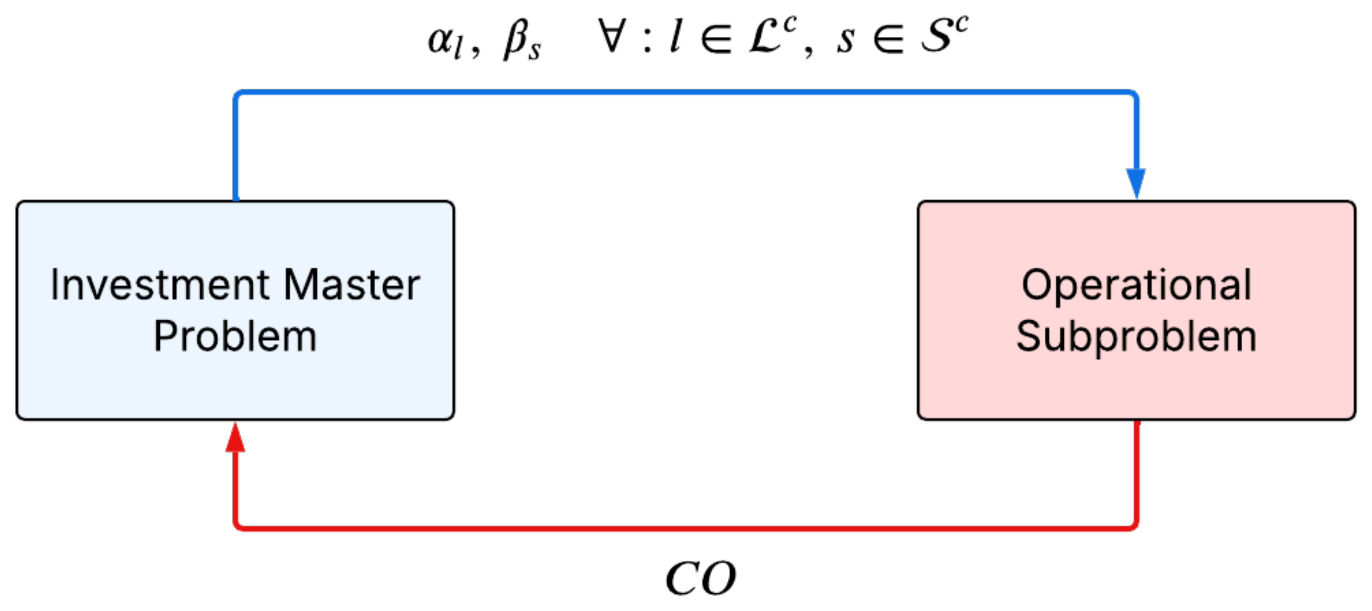
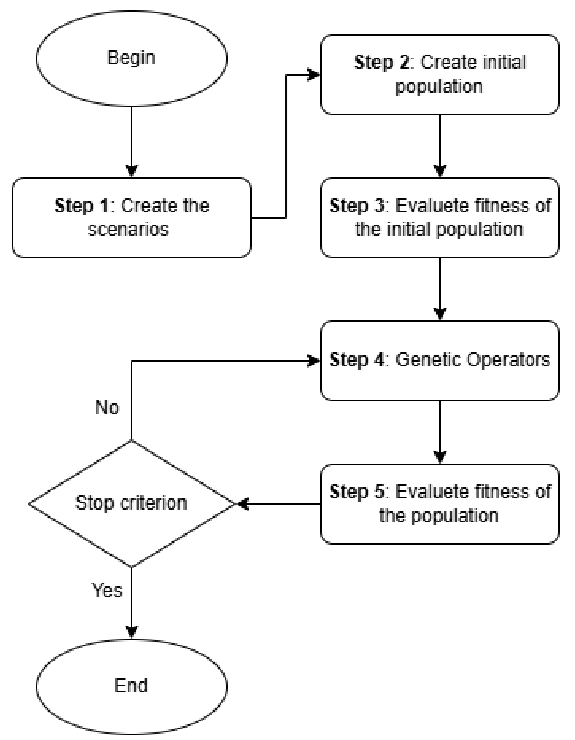
4. Solution Strategy

To address the mixed-integer nonlinear problem, this work proposes a decomposition strategy that separates it into an investment master problem and an operational subproblem.
The investment master problem determines the optimal investment decisions by defining the integer investment variables for transmission lines α l , l L c and energy storage devices β s , s S c .
The operational subproblem evaluates the operational cost of the system ( C O ) in all scenarios over a one-year horizon. This cost is then fed back into the investment master problem to iteratively refine investment decisions. The operational subproblem solves the network-constrained unit commitment for each scenario, treating the investments determined by the master problem as implemented. Specifically, transmission lines and storage devices with positive investment values ( α l > 0 or β s > 0 ) are incorporated into the sets of existing transmission lines ( L e ) and storage systems ( S e ).
This decomposition eliminates the nonlinearity of the original problem, allowing an iterative solution process between the investment master problem and the operational subproblem. The investment problem is solved using a genetic algorithm-based optimization approach, while the operational subproblem is addressed with commercial MILP solvers. Figure 1 illustrates the process.

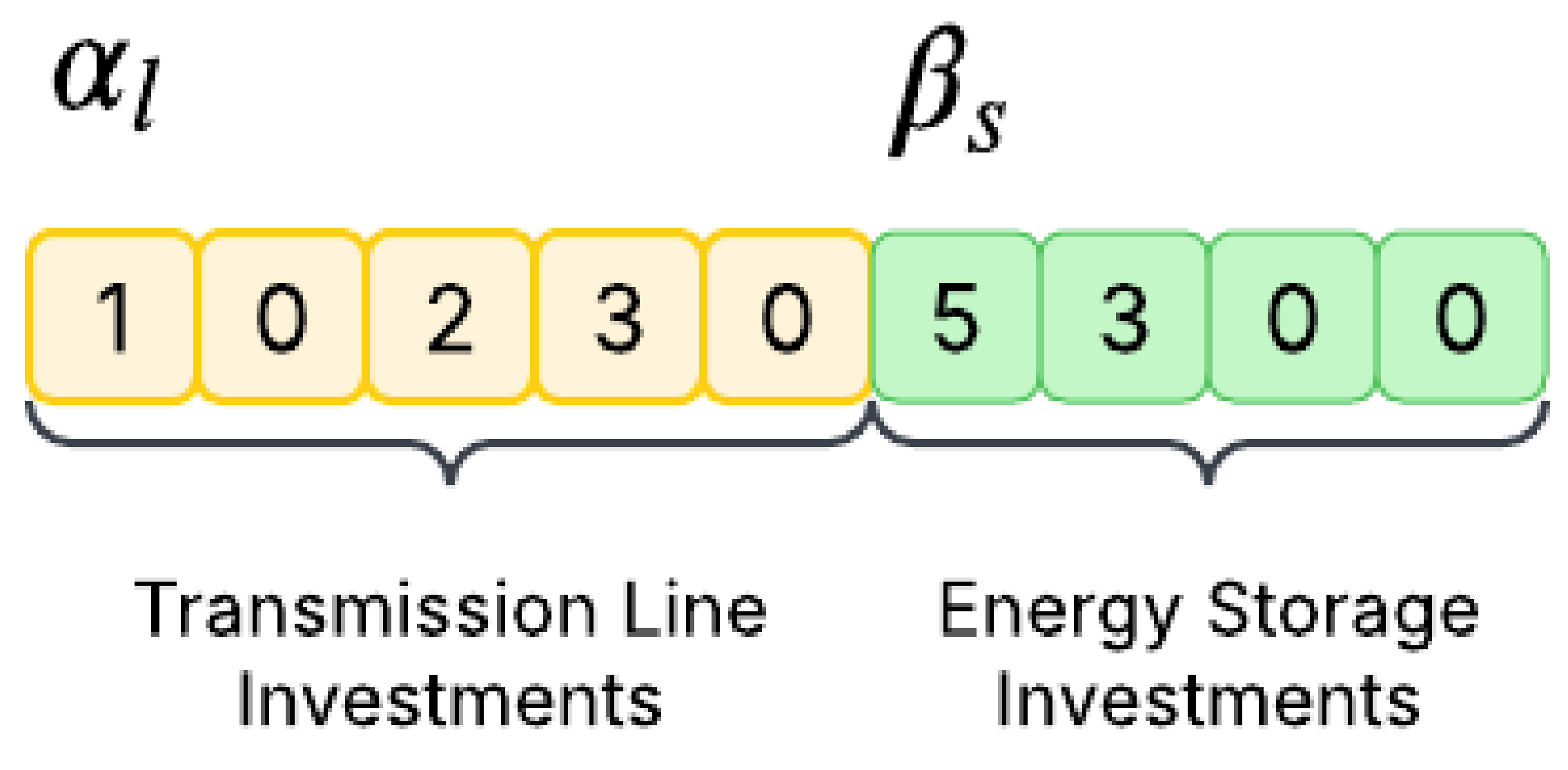
4.1. Investment Master Problem

The genetic algorithm used in this study employs four main operators: selection, crossover, mutation, and elitism.
Each chromosome (individual) consists of two independent segments: one for transmission line investments and another for storage system investments. Figure 2 illustrates a chromosome representation for a fictitious system with five candidate branches for transmission expansion and four candidate buses for the installation of energy storage. In this example, the chromosome specifies the construction of one transmission line on the first candidate branch, two lines on the third, and three lines on the fourth. Similarly, it indicates investments in five storage units at the first candidate bus and three at the second.
To maintain structural integrity, crossover and mutation operations are applied separately within each segment (transmission line investment or energy storage investment). This prevents infeasible solutions caused by swapping genes between unrelated components since the upper limits A l m a x and B s m a x may differ depending on the system under analysis.
The crossover process is modified to occur exclusively within each segment. This prevents transmission line investments from being swapped with storage investments, preserving chromosome integrity, and eliminating the risk of infeasible solutions.
Mutation operator adjustments are made so that random alterations affect only one category at a time (transmission, storage, or both). This ensures that mutations adhere to system constraints, preventing structural inconsistencies.
The fitness value of each chromosome is computed after solving the operational subproblem. It corresponds to the sum of the four cost components in the original objective function (1) plus a penalty cost C P E . A lower fitness value indicates a better performing chromosome relative to others.
The penalty cost is applied when the operational subproblem is infeasible for any scenario analyzed. To strongly discourage insufficient investment solutions, a high penalty value USD 10 12 is used.
Figure 3 illustrates the step-by-step procedure of the proposed methodology.
Step 1: Representative day scenarios for wind generation and load demand are created using a clustering algorithm. These scenarios are used to model the uncertainties in the system.
Step 2: An initial population of candidate solutions (chromosomes) is randomly generated. Each chromosome represents a possible investment plan, including the expansion of transmission lines and energy storage systems.
Step 3: The fitness of each chromosome in the initial population is evaluated based on its total investment and operational cost, obtained by solving a unit commitment problem.
Step 4: Genetic operators, selection, crossover, mutation, and elitism are applied to evolve the population.
Step 5: The fitness of the new population is evaluated, following the same procedure as in Step 3.
The algorithm then checks whether the stopping criterion has been met (e.g., the maximum number of iterations or convergence threshold). If the criterion is satisfied, the algorithm terminates; otherwise, it returns to Step 4 to continue the evolutionary process.
This approach allows for efficient exploration of the large combinatorial search space associated with co-expansion planning while ensuring high-quality solutions.

4.2. Operational Subproblem

The operational subproblem receives investment decisions from the investment master problem, specifically the integer investment variables for transmission lines ( α l , l L c ) and energy storage devices ( β s , s S c ). Transmission lines and storage devices with positive investment values ( α l > 0 or β s > 0 ) are incorporated into the sets of existing transmission lines ( L e ) and storage systems ( S e ).
Based on these decisions, the operational subproblem is formulated as a stochastic network-constrained unit commitment model, represented as a mixed-integer linear optimization problem. The objective is to minimize the annual operational cost while accounting for uncertainties in wind generation and electricity demand. A set of representative daily scenarios is considered, where each scenario ϕ is assigned a probability weight γ ϕ , reflecting its probability of occurrence over the year.
The mathematical formulation of the stochastic network-constrained unit commitment model is presented below.
min C O = 365 ϕ Φ γ ϕ { h H [ g G b g · p g h ϕ t h e + a g · u g h ϕ t h e + s S μ · p s h ϕ c h a + p s h ϕ d i s + w W η · p w h ϕ c u r ] }
subject to (8), (9), (11), (13)–(26), (28), (30), (32), and (35).

5. Simulations

This section presents the results obtained using the proposed methodology on a modified IEEE-RTS 24-bus test system [20]. The system comprises 24 buses and 41 candidate branches for expansion. Each branch can accommodate up to three transmission lines. The investment costs for the candidate lines of 230 kV and 132 kV are USD 120,000.0/km and USD 70,000.0/km, respectively [20].
The load profile and the technical data of the thermal generation units were obtained from [20,21]. Table 2 summarizes the main characteristics of these units. The original system data presented in [20,21] are not suitable for long-term planning. To accommodate a long-term planning approach, the capacities of all existing transmission lines are reduced to one-third of their original values, following [2]. In addition, the maximum thermal generator capacity and up-ramp limit are doubled.
The system includes three wind farms located at buses 20, 21, and 23, with maximum generation capacities of 900.0 MW, 600.0 MW, and 300.0 MW, respectively. Following [22], the generation cost of these wind farms is set to zero. The curtailment cost of wind generation is adopted as USD 80/MW, as used in [23].
Energy storage investments are considered at buses 5, 6, 8, 10, 11, and 14, following [15]. Each bus can accommodate up to five storage units, with each unit having a power capacity of 100 MW and an energy capacity of 500 MWh. The subsidized costs are set at USD 500.0/kW (power) and USD 20.0/kWh (energy), as used in [8]. The charging and discharge efficiencies of the energy storage device are 95%. Investment costs are annualized using an interest rate 5%, with assumed lifetimes of 60 years for transmission lines [8,15] and 20 years for storage devices [15]. The maximum number of energy storage devices that can be invested at each bus is five.
The study analyzes five representative daily scenarios to capture hourly variations in demand and wind generation at the three wind farms. These scenarios are derived from historical load and wind generation data [24]. The k-means clustering technique is applied to group the data and assign weighted probabilities to each scenario. The complete system data and scenarios are available in [25].
Two case studies are investigated:
  • Case A: Investments in transmission line.
  • Case B: Investments in transmission line and energy storage device.
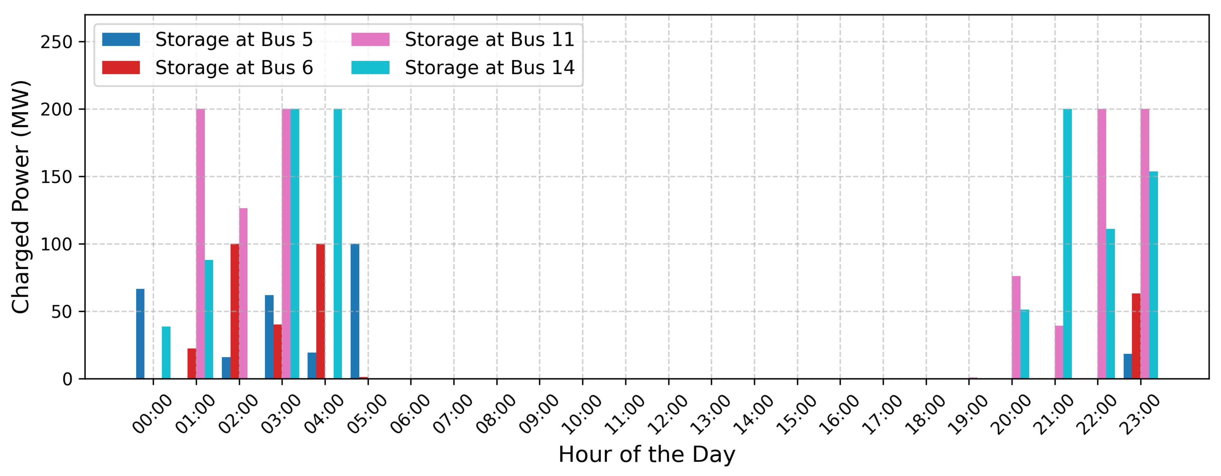
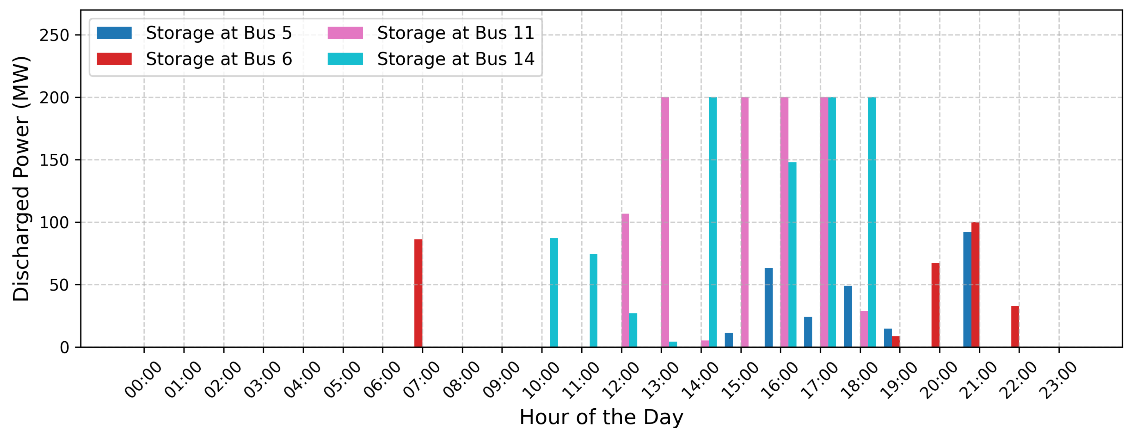
The parameters of the genetic algorithm are presented in Table 3. These parameters were defined empirically. For all cases, the convergence criterion is the maximum number of iterations. Ten simulations were conducted for each case defined in the following. All simulations were performed on a 2.7 GHz Intel® Core i7 processor, with the codes implemented in MATLAB® software version R2015a.

Results

Table 4 summarizes the the best investment investment decisions obtained for each planning case. The table presents the total investment costs, disaggregated into transmission and storage components, as well as the corresponding annual operating costs under uncertainty. In addition, it details the specific transmission lines selected for expansion and the location and the number of ESS units installed in Case B.
For Case A, the optimal solution includes a transmission line investment cost of USD 1494.0 M, involving the construction of one line between buses 2–6, 3–9, 4–9, 6–10, 7–8, 9–12, 12–23, 14–16, 15–16, 16–17, 18–21, 20–23, and 14–23. In addition, two transmission lines are constructed between buses 1–5, 9–11, 11–14, 12–13, 17–22, and 1–8, while three lines are added between buses 6–7. The corresponding annual operational cost is USD 42,702.86 M.
For Case B, the optimal solution involves a transmission line investment cost of USD 1,193.00 M and an energy storage investment of USD 136.00 M. The transmission expansion plan suggests building new lines between buses 2–6, 3–9, 3–24, 4–9, 5–10, 6–10, 8–9, 9–11, 10–11, 11–14, 12–23, 14–16, 15–21, 15–24, 16–17, 17–18, 17–22, 20–23, and 13–14, along with the addition of two transmission lines between buses 1–5, 7–8, 1–8, and 14–23.
The investment in energy storage includes the installation of one storage unit at bus 5, one unit at bus 6, and two storage units at buses 11 and 14. This combined investment in transmission lines and energy storage results in an annual operating cost of USD 81 .60 M.
It is evident that Case B presents a more cost-effective transmission expansion plan compared to Case A, with a cost reduction of 20.15%. The total expansion cost in Case B, including both transmission line and energy storage investments USD 1274.6 M, remains 14.69% lower than the transmission expansion cost in Case A. Additionally, the annual operating cost of Case B is 26.19% lower than that of Case A. These results highlight the economic benefits of considering the co-expansion planning of transmission lines and energy storage devices.
Table 5 summarizes the best solutions obtained for each case, including the stochastic thermal generation, energy charged, energy discharged, and wind curtailment. These values are calculated by summing the total output for each scenario, multiplying by the probability of the scenario, and then aggregating the results across all five scenarios.
The stochastic thermal generation and wind curtailment in Case B are both lower than in Case A. Specifically, Case B reduces thermal generation by 87.25 MWh compared to Case A, which translates to an annual reduction of 31,846.25 MWh. Additionally, Case B decreases wind curtailment by 360.32 MWh, equivalent to 131,516.8 MWh of avoided wind curtailment per year. This reduction is primarily due to the presence of energy storage systems, which decrease the dependence on thermal generation by enhancing operational flexibility and enabling a more cost-effective dispatch of thermal units while adhering to unit commitment constraints. Furthermore, storage systems mitigate wind curtailment by storing surplus wind energy and discharging it when it is most economically beneficial to the system. As a result, Case B achieves a 91.99% reduction in curtailed wind energy compared to Case A.
Table 6 and Table 7 present the optimal dispatch of the thermal generator units for each hour of the first scenario, corresponding to the best solution found for Case A and Case B, respectively. These tables demonstrate that the model complies with unit commitment constraints, thus validating the effectiveness of the proposed methodology. It can be observed that the operational profiles of the thermal units differ significantly between the two cases. In Case A, the thermal units operate at a total cost of USD 135.484 M, whereas in Case B, the operation cost is reduced to USD 105.936 M. This indicates that the joint expansion of transmission lines and energy storage systems leads to a reduction in the operational cost of thermal generation by approximately 21.81%, highlighting the economic benefits of co-expansion planning.
Figure 4 and Figure 5 present the charge and discharge output for the first scenario of the energy storage devices invested in Case B. The Y-axis in Figure 4 shows the charging power (MW) of each ESS, while the Y-axis in Figure 5 represents the amount of power discharged into the grid. The X-axis in both figures corresponds to the time of day (hours). It can be observed that energy storage systems follow a charging pattern during the early hours of the day (00:00–05:00) and late night (20:00–23:00), periods when demand is lower. In contrast, discharge occurs primarily in the afternoon (12:00–19:00), aligning with the period of higher load demand.

6. Conclusions

This paper proposed a methodology for the co-expansion planning of transmission lines and energy storage systems, incorporating demand and wind generation uncertainties through representative day scenarios and including unit commitment constraints for thermal generators to reflect realistic operational dynamics. The problem was formulated as a mixed-integer nonlinear program and solved using a decomposition approach that combines genetic algorithms with classical optimization techniques.
The results demonstrate that co-planning leads to significant economic benefits compared to transmission-only expansion. Specifically, the proposed approach achieved a 14.69% reduction in total expansion costs, a 26.19% decrease in annual operational costs, and a 91.99% reduction in wind curtailment, highlighting the synergy between transmission expansion and ESS investments. These improvements are primarily due to the improved system flexibility provided by storage, which reduces dependence on thermal generation and improves the integration of renewable energy.
The results highlight the interdependence between transmission expansion and energy storage investments, as well as their impact on market indices. Furthermore, the findings indicate that co-planning transmission lines and energy storage devices leads to greater economic efficiency, reducing both investment and operational costs compared to planning transmission expansion alone.

Future Work

Future research will aim to enhance the realism and applicability of the proposed framework through the following extensions:
  • Integration of hydroelectric power plants, introducing long-term storage capabilities and seasonal planning aspects;
  • Expansion of the formulation to include AC power flow constraints, improving the electrical accuracy of the model;
  • Application of the methodology to larger test systems, allowing for evaluation of scalability and computational performance.

Author Contributions

Conceptualization, E.J.d.O. and L.S.N.; methodology, E.J.d.O. and L.S.N.; software, L.S.N.; validation, E.J.d.O. and L.S.N.; formal analysis, E.J.d.O., L.S.N., L.W.d.O. and A.N.d.P.; investigation, L.S.N.; writing—original draft preparation, E.J.d.O. and L.S.N.; writing—review and editing, E.J.d.O., L.S.N., L.W.d.O. and A.N.d.P.; supervision, E.J.d.O.; project administration, E.J.d.O. and L.S.N. All authors have read and agreed to the published version of the manuscript.

Funding

This research received no external funding.

Institutional Review Board Statement

Not applicable.

Informed Consent Statement

Not applicable.

Data Availability Statement

The required data are provided in the paper.

Acknowledgments

The authors gratefully acknowledge the Brazilian agency for the financial support in part of the Brazilian Federal Agency for the Support and Evaluation of Graduate Education (CAPES), the National Research Council (CNPq), the Brazilian Institute of Science and Technology (INERGE), and the State of Minas Gerais Research Foundation (FAPEMIG). The authors also express gratitude for the educational support of the Federal University of Juiz de Fora (UFJF).

Conflicts of Interest

The authors declare no conflicts of interest.

Abbreviations

gIndex of generating units
hIndex of time periods
ϕ Index of scenarios or phases
i , j Indexes of buses
lIndex of transmission lines
sIndex of storage units
wIndex of wind units
G Set of generating units
H Set of time periods
Φ Set of scenarios or phases
B Set of buses
L E Set of existing transmission lines
L C Set of candidate transmission lines
S Set of storage units
S E Set of existing storage units
S C Set of candidate storage units
W Set of wind units
P g t h e , m i n Minimum power output of thermal unit g
P g t h e , m a x Maximum power output of thermal unit g
R U g Ramp-up limit of thermal unit g
R D g Ramp-down limit of thermal unit g
S U g Startup ramp limit of thermal unit g
S D g Shutdown ramp limit of thermal unit g
U T g Minimum up-time of thermal unit g
D T g Minimum down-time of thermal unit g
G g Number of initial periods thermal unit g must be online
L g Number of initial periods thermal unit g must be offline
TTotal number of time periods
D i h ϕ Load demand at bus i in period h and scenario ϕ
f l m a x Maximum power flow limit of transmission line l
x l Reactance of transmission line l
θ m a x Maximum bus angle limit
Z s m i n Minimum state of charge (SOC) of storage unit s
Z s m a x Maximum state of charge (SOC) of storage unit s
P s d i s , m i n Minimum discharge power of storage unit s
P s d i s , m a x Maximum discharge power of storage unit s
P s c h a , m i n Minimum charge power of storage unit s
P s c h a , m a x Maximum charge power of storage unit s
σ s d i s Discharge efficiency of storage unit s
σ s c h a Charge efficiency of storage unit s
P w h ϕ w i d Available wind power of wind unit w in period h and scenario ϕ
C l T L Investment cost of transmission line l
C s S E Energy component of the investment cost for storage unit s
C s S P Power component of the investment cost for storage unit s
rDiscount rate
Y l Lifetime of transmission line l
Y s Lifetime of storage unit s
a g Fixed cost of operating thermal unit g (USD)
b g Variable cost of operating thermal unit g (USD/MW)
μ Operational cost of storage units (USD/MW)
η Curtailment cost of wind generation (USD/MWh)
γ ϕ Weight of scenario ϕ
u g h ϕ t h e Binary variable indicating if thermal unit g is online (1) or offline (0) in period h and scenario ϕ
p g h ϕ t h e Power output of thermal unit g in period h and scenario ϕ
ρ g h ϕ t h e Maximum available power output of thermal unit g in period h and scenario ϕ
f l h ϕ Power flow in transmission line l in period h and scenario ϕ
θ i h ϕ Voltage angle at bus i in period h and scenario ϕ
z s h ϕ State of charge (SOC) of storage unit s in period h and scenario ϕ
p s h ϕ d i s Discharge power of storage unit s in period h and scenario ϕ
p s h ϕ c h a Charge power of storage unit s in period h and scenario ϕ
p w h ϕ c u r Curtailed wind power of wind unit w in period h and scenario ϕ
α l Binary variable indicating if candidate transmission line l is built
β s Binary variable indicating if candidate storage unit s is built
TNEPTransmission Network Expansion Planning
ESSEnergy Storage System
CETESCo-expansion planning of transmission lines and energy storage devices
UCUnit Commitment
GESSGeneric Energy Storage System
BESSBattery Energy Storage System
CAESCompressed Air Energy Storage
PHESPumped Hydro Energy Storage
MILPMixed-Integer Linear Programming
CCGColumn-and-Constraint Generation
GAGenetic Algorithm

References

  1. Hu, Z.; Zhang, F.; Li, B. Transmission expansion planning considering the deployment of energy storage systems. In Proceedings of the 2012 IEEE Power and Energy Society General Meeting, San Diego, CA, USA, 22–26 July 2012; IEEE: Piscataway, NJ, USA, 2012; pp. 1–6. [Google Scholar]
  2. Zhang, F.; Hu, Z.; Song, Y. Mixed-integer linear model for transmission expansion planning with line losses and energy storage systems. IET Gener. Transm. Distrib. 2013, 7, 919–928. [Google Scholar] [CrossRef]
  3. Hedayati, M.; Zhang, J.; Hedman, K.W. Joint transmission expansion planning and energy storage placement in smart grid towards efficient integration of renewable energy. In Proceedings of the 2014 IEEE PES T&D Conference and Exposition, Chicago, IL, USA, 14–17 April 2014; IEEE: Piscataway, NJ, USA, 2014; pp. 1–5. [Google Scholar]
  4. MacRae, C.; Ernst, A.; Ozlen, M. A Benders decomposition approach to transmission expansion planning considering energy storage. Energy 2016, 112, 795–803. [Google Scholar] [CrossRef]
  5. Qiu, T.; Xu, B.; Wang, Y.; Dvorkin, Y.; Kirschen, D.S. Stochastic multistage coplanning of transmission expansion and energy storage. IEEE Trans. Power Syst. 2016, 32, 643–651. [Google Scholar] [CrossRef]
  6. Falugi, P.; Konstantelos, I.; Strbac, G. Planning with multiple transmission and storage investment options under uncertainty: A nested decomposition approach. IEEE Trans. Power Syst. 2017, 33, 3559–3572. [Google Scholar] [CrossRef]
  7. Aguado, J.; de La Torre, S.; Triviño, A. Battery energy storage systems in transmission network expansion planning. Electr. Power Syst. Res. 2017, 145, 63–72. [Google Scholar] [CrossRef]
  8. Dvorkin, Y.; Fernández-Blanco, R.; Wang, Y.; Xu, B.; Kirschen, D.S.; Pandžić, H.; Watson, J.P.; Silva-Monroy, C.A. Co-planning of investments in transmission and merchant energy storage. IEEE Trans. Power Syst. 2017, 33, 245–256. [Google Scholar] [CrossRef]
  9. Zhang, X.; Conejo, A.J. Coordinated investment in transmission and storage systems representing long-and short-term uncertainty. IEEE Trans. Power Syst. 2018, 33, 7143–7151. [Google Scholar] [CrossRef]
  10. Nikoobakht, A.; Aghaei, J. Integrated transmission and storage systems investment planning hosting wind power generation: Continuous-time hybrid stochastic/robust optimisation. IET Gener. Transm. Distrib. 2019, 13, 4870–4879. [Google Scholar] [CrossRef]
  11. Wang, S.; Geng, G.; Jiang, Q. Robust co-planning of energy storage and transmission line with mixed integer recourse. IEEE Trans. Power Syst. 2019, 34, 4728–4738. [Google Scholar] [CrossRef]
  12. Gan, W.; Ai, X.; Fang, J.; Yan, M.; Yao, W.; Zuo, W.; Wen, J. Security constrained co-planning of transmission expansion and energy storage. Appl. Energy 2019, 239, 383–394. [Google Scholar] [CrossRef]
  13. Luburić, Z.; Pandžić, H.; Carrión, M. Transmission expansion planning model considering battery energy storage, TCSC and lines using AC OPF. IEEE Access 2020, 8, 203429–203439. [Google Scholar] [CrossRef]
  14. Mazaheri, H.; Abbaspour, A.; Fotuhi-Firuzabad, M.; Moeini-Aghtaie, M.; Farzin, H.; Wang, F.; Dehghanian, P. An online method for MILP co-planning model of large-scale transmission expansion planning and energy storage systems considering N-1 criterion. IET Gener. Transm. Distrib. 2021, 15, 664–677. [Google Scholar] [CrossRef]
  15. de Oliveira, E.J.; de Paula, A.N.; de Oliveira, L.W.; Honório, L.d.M. Block-Based Multicut Benders Decomposition Algorithm for Transmission and Energy Storage Co-Planning. Int. Trans. Electr. Energy Syst. 2022, 2022. [Google Scholar] [CrossRef]
  16. Carrión, M.; Arroyo, J.M. A computationally efficient mixed-integer linear formulation for the thermal unit commitment problem. IEEE Trans. Power Syst. 2006, 21, 1371–1378. [Google Scholar] [CrossRef]
  17. Dillon, T.S.; Edwin, K.W.; Kochs, H.D.; Taud, R. Integer programming approach to the problem of optimal unit commitment with probabilistic reserve determination. IEEE Trans. Power Appar. Syst. 1978, PAS-97, 2154–2166. [Google Scholar] [CrossRef]
  18. Arroyo, J.M.; Conejo, A.J. Optimal response of a thermal unit to an electricity spot market. IEEE Trans. Power Syst. 2000, 15, 1098–1104. [Google Scholar] [CrossRef]
  19. Morales-España, G.; Latorre, J.M.; Ramos, A. Tight and compact MILP formulation for the thermal unit commitment problem. IEEE Trans. Power Syst. 2013, 28, 4897–4908. [Google Scholar] [CrossRef]
  20. Subcommittee, P.M. IEEE reliability test system. IEEE Trans. Power Appar. Syst. 1979, PAS-98, 2047–2054. [Google Scholar] [CrossRef]
  21. Ordoudis, C.; Pinson, P.; Morales, J.M.; Zugno, M. An Updated Version of the IEEE RTS 24-Bus System for Electricity Market and Power System Operation Studies; Technical University of Denmark: Kongens Lyngby, Denmark, 2016; Volume 13. [Google Scholar]
  22. de Paula, A.N.; de Oliveira, E.J.; de Oliveira, L.W.; Honório, L.M. Robust static transmission expansion planning considering contingency and wind power generation. J. Control Autom. Electr. Syst. 2020, 31, 461–470. [Google Scholar] [CrossRef]
  23. Fernández-Blanco, R.; Dvorkin, Y.; Xu, B.; Wang, Y.; Kirschen, D.S. Optimal energy storage siting and sizing: A WECC case study. IEEE Trans. Sustain. Energy 2016, 8, 733–743. [Google Scholar] [CrossRef]
  24. Merrick, J.H. On representation of temporal variability in electricity capacity planning models. Energy Econ. 2016, 59, 261–274. [Google Scholar] [CrossRef]
  25. Nepomuce, L.; de Oliveira, E.; de Oliveira, L.; de Paula, A. Data for paper: A Novel Framework for Co-Expansion Planning of Transmission Lines and Energy Storage Devices Considering Unit Commitment. 2025. Available online: https://drive.google.com/drive/folders/1jJZeTsX8kTKbMI_zjHbBncBdxizD9wer?usp=drive_link (accessed on 21 May 2025).
Figure 1. Flowchart of the solution strategy.
Technologies 13 00241 g001
Figure 2. Chromosome encoding.
Technologies 13 00241 g002
Figure 3. Step-by-step flowchart of the proposed methodology.
Technologies 13 00241 g003
Figure 4. Charge operation of energy storage systems for Case B —First scenario.
Technologies 13 00241 g004
Figure 5. Discharge operation of energy storage systems for Case B —First scenario.
Technologies 13 00241 g005
Table 1. Taxonomy of recent publications that propose methodologies for solving co-planning of transmission and storage devices.
ReferenceUncertaintiesPlanning
Horizon
UCNetwork
Representation
Storage
Investment
TechnologySistemaModel
 [1]NoSNoLossless DCBGESSGarver 6-bus
IEEE 24-bus
Brazil 46-bus
MILP
Solver
[2]NoSNoDCBGESSGarver 6-bus
IEEE 24-bus
MILP
Solver
[3]NoDNoLossless DCBBESSRoy Billinton 6-bus
IEEE 24-bus
MILP
Solver
[4]NoSNoLossless DCCGESSGarver 6-bus
IEEE 24-bus
Brazil 46-bus
Benders
Decomposition
[5]YesDYesLossless DCCBESSIEEE 24-bus
IEEE 118-bus
MILP
Solver
[6]NoDNoLossless DCBBESS
CAES
PHES
IEEE 118-busNested Benders
Decomposition
[7]YesSNoDCBBESSGarver 6-bus
IEEE 24-bus
MILP
Solver
[8]YesSNoLossless DCCBESSWECC system 240-busCCG
[9]YesSNoLossless DCBGESSIEEE 24-busBenders
Decomposition
[10]YesSNoLossless DCBGESSIEEE 24-busBenders
Decomposition
[10]YesSNoLossless DCBGESSIEEE 24-busBenders
Decomposition
[11]YesSNoLossless DCCBESSGarver 6-bus
Chinese 196-bus
CCG
[12]YesDNoLossless DCBBESS
PHES
Garver 6-bus
Gansu-53 bus
Benders
Decomposition
[13]NoSNoACCBESSIEEE 24-busBenders
Decomposition
[14]NoSNoLossless DCBCAESGarver 6-bus
IEEE 24-bus
MILP
Solver
[15]YesSNoLossless DCBBESSGarver 6-bus
IEEE 24-bus
IEEE 118-bus
Benders
Decomposition
This WorkYesSYesLossless DCBGESSIEEE 24-busDecomposition
GA
MILP Solver
Table 2. Data of the thermal generator units.
UnitBus P g max P g min R U g R D g U T g D T g P 0 g u 0 g G g L g a g b g c g C S U g C S D g S U g S D g
11152.0030.40120.00120.008476.0012200.0113.32108.001430.40715.20152.00152.00
22152.0030.40120.00120.008476.0012200.0713.32108.001430.40715.20152.00152.00
37350.0075.00350.00350.00880.000020.0020.70118.001725.00862.50300.00300.00
413591.00206.85240.00240.0012100.000010.0120.9394.003056.701528.35591.00591.00
51560.0012.0060.0060.00420.000010.0326.1184.00437.00218.5060.0060.00
615155.0054.25155.00155.00880.000020.0110.52118.00312.00156.0089.2089.20
716155.0054.25155.00155.0088124.0011000.0110.52118.00312.00156.0089.2089.20
818400.00100.00280.00280.0011240.0015000.036.02177.000.000.00240.00240.00
921400.00100.00280.00280.0011240.0011600.035.47177.000.000.00240.00240.00
1022300.00300.00300.00300.0011240.0012400.012.00177.000.000.00300.00300.00
1123310.00108.50180.00180.0088248.0011000.0110.52118.00624.00312.00178.50178.50
1223350.00140.00240.00240.0088280.0015000.0110.89118.002298.001149.00210.00210.0
Table 3. Parameters of the genetic algorithm.
ParametersValue
Number of chromosomes20
Maximum number of iterations50
Crossover rate0.7
Mutation rate0.3
Number of tournament participants4
Size of the elite set2
Table 4. Best solution for each case—part 1.
CaseTotal Investment
Cost in Lines
(USD/M)
Total Investment
Cost in Storage
(USD/M)
Annual
Operational
Cost (USD/M)
Transmission
Expansion
Storage
Expansion
A1494.0-42,702.861–5 (2), 2–6, 3–9, 4–9, 6–10, 7–8,
9–11 (2), 9–12, 11–14 (2), 12–13 (2), 12–23,
14–16, 15–16, 16–17, 17–22 (2), 18–21,
20–23, 1–8 (2), 6–7 (3), 14–23
B1193.0081.6031,520.561–5 (2), 2–6, 3–9, 3–24, 4–9, 5–10,
6–10, 7–8 (2), 8–9, 9–11, 10–11, 11–14,
12–23, 14–16, 15–21, 15–24, 16–17, 17–18,
17–22, 20–23, 1–8 (2), 13–14, 14–23 (2)
5 (1), 6 (1),
11 (2), 14 (2)
Table 5. Best solution for each case—part 2.
CaseStochastic
Thermal Generation
(MWh)
Stochastic
Energy Charged
(MWh)
Stochastic
Energy Discharged
(MWh)
Stochastic
Wind Curtailment
(MWh)
A43,171.06--391.72
B43,083.812800.792527.7231.40
Table 6. Power generation schedule of the optimal solution for Case A —First scenario.
HourPower Generation of Units (MW)
1197.6730.40000054.250101.25600.00108.50140.00
2133.1930.40000054.250102.57600.000140.00
390.4430.400000100.4000600.000140.00
474.4230.40000094.6800600.000140.00
577.6430.40000054.250100.00572.260140.00
6112.0030.40000054.25172.210600.000140.00
7290.9259.88000054.25479.540600.000169.49
8304.00216.76000054.25548.090600.000363.13
9304.00278.2775.0000054.25593.200600.000543.89
10304.00286.44125.6400058.51635.420600.000629.94
11304.00291.65183.8900083.65666.230600.000656.30
12304.00293.57205.3600092.39686.240600.000680.72
13304.00297.49249.21000112.70698.560600.000691.21
14304.00301.18290.40000132.23706.280600.000693.36
15304.00300.87286.99000130.90701.810600.000687.63
16304.00303.12312.10000143.34700.740600.000684.49
17304.00265.65499.92000201.23710.520600.000682.46
18304.00248.98544.69000211.25700.820600.000666.64
19304.00250.80539.80000214.74647.020600.000595.51
20304.00304.00354.63000173.22572.580600.000510.10
21304.00296.48236.6900089.20492.860600.000435.96
22304.00222.3375.000000416.730600.000371.06
23253.7440.3275.000000300.580600.000140.00
24109.81075.000000125.790600.0000
Table 7. Power generation schedule of the optimal solution for Case B —First scenario.
HourPower Generation of Units (MW)
123456789101112
130.4030.40000054.250373.36600.00108.50140.00
230.4030.40000000601.29600.00108.500
330.4030.40000000434.06600.00108.500
473.4230.40000000628.96600.00108.500
530.4030.40000000524.33600.00108.500
630.4030.40000000440.52600.00108.500
759.0730.40000000722.64600.00241.960
881.4930.4000000100.00788.85600.00399.290
9302.1171.9700000150.39800.00600.00524.160
10304.00129.3700000186.60800.00600.00619.980
11230.15232.7500000215.68800.00600.00620.000
12282.37258.9600000226.42800.00600.00620.000
13304.00268.9800000226.47800.00600.00620.000
14304.00268.3000000230.92800.00600.00620.000
15304.00269.5200000213.57800.00600.00620.000
16304.00271.9300000240.66800.00600.00620.000
17304.00287.8200000241.26800.00600.00620.000
18304.00276.0800000252.16800.00600.00620.000
19304.00285.7200000264.52800.00600.00620.000
20304.00273.3000000198.99800.00600.00620.000
21304.00152.0000000132.26800.00600.00526.890
22147.71000000100.00800.00558.74429.900
23171.290000000747.20591.09178.500
24139.230000000608.18597.8700
Disclaimer/Publisher’s Note: The statements, opinions and data contained in all publications are solely those of the individual author(s) and contributor(s) and not of MDPI and/or the editor(s). MDPI and/or the editor(s) disclaim responsibility for any injury to people or property resulting from any ideas, methods, instructions or products referred to in the content.

