1. Introduction
Driven by the global energy transformation and the “double carbon” strategy, the volatility of renewable energy poses a serious challenge to the stability of power systems (IEA, 2023) [
1]. In 2024, the global installed capacity of renewable energy exceeded 650 gw [
2], but its random fluctuation characteristics (such as the intraday fluctuation of wind power up to 40% [
3]) pose a serious challenge to the supply and demand balance and stable operation of the power system. Accurate power load forecasting is the core link to improve the stability of the system. It needs to take into account the nonlinear coupling characteristics of high-dimensional spatiotemporal data (weather, electricity price, historical load, etc.) and the transparency requirements of the decision-making process. However, the traditional methods face multiple bottlenecks: physical models rely on Simplified assumptions (such as load temperature linear response [
4], which cannot characterize the inhibitory effect of high temperature and electricity price linkage on loads), statistical models (such as ARIMA) are limited by stationarity assumptions [
5] (difficult to handle non-stationary load changes after renewable energy grid integration), and machine learning models (such as SVM) have dimensional disaster problems [
6] (significantly reduced ability to model high-dimensional features). Although the hybrid model (e.g., Zeng Jinhui [
7] improved the accuracy by 12.3% based on empirical mode decomposition and improved LSTM, and Zhao Yiran [
8] combined seasonal decomposition and CNN-BiLSTM to reduce the error by 8.7%) improved the accuracy through multi technology fusion, there are still two key defects: first, the decoupling processing of spatiotemporal features leads to the loss of associated information. For example, although the multi model fusion method (such as CNN-LSTM-XGBoost [
9] and application ensemble empirical mode decomposition [
10]) can improve the prediction accuracy, it does not effectively solve the problem of independent processing of spatiotemporal features (such as the inability to capture the synergistic impact of electricity price fluctuations on loads during high temperature periods). Second, the model decision-making process lacks transparency, and the “black box” feature makes it difficult to quantify the influence mechanism of key factors such as electricity price and weather (such as the quantitative relationship between electricity price fluctuations and load changes), which seriously restricts its trust in power dispatching [
11].
Deep learning technology provides a new path for load forecasting. CNNs are good at extracting local spatial features [
12] (such as temporal window correlation patterns in meteorological data), BiLSTM models can capture the time-dependent relationship [
13] (such as the correlation between fluctuations in load sequences), and the self-attention mechanism can improve the prediction accuracy by focusing on key information [
14,
15]. The graph neural network (GNN) shows its potential in network structure modeling. For example, reference [
16] uses state theory and reciprocity to embed and optimize social network nodes to express learning. Its ability to explicitly model spatial dependence provides a new idea for power system load forecasting. However, the existing GNN model in the power field (such as the graph convolution load forecasting method in reference [
17]) relies on structured graph data, such as grid node connections, and needs to map unstructured features such as meteorology and electricity price (such as continuously changing meteorological data, real-time electricity price, and other non-tabular data) to graph node attributes, resulting in a 12–15% loss of key event features [
11] (such as high-frequency information such as sudden changes in electricity prices that are difficult to fully preserve due to dimensionality compression). In addition, the complexity of the graph convolution operation increases exponentially with the number of nodes (the time-consuming 100 node scenario is three times more time consuming than a CNN [
18]), which is difficult to adapt to the real-time processing requirements of high-dimensional spatiotemporal data.
However, the existing studies focus more on accuracy improvement and pay less attention to interpretability. For example, although the multiscale CNN BiLSTM attention model proposed by Ouyang Fulian et al. [
19] improves local feature extraction through multiscale convolution, it uses a static attention weight, which leads to insufficient dynamic focusing ability for non-periodic events such as sudden electricity price changes and extreme weather (with a prediction error increase of about 9% in similar extreme scenarios), and it is difficult to capture the transient nonlinear changes in the load response. The parallel multi-channel CNN BiLSTM structure proposed by Hasanat et al. (2024) [
20] has verified the effectiveness of spatiotemporal feature decoupling, but it lacks a unified feature importance evaluation mechanism and is unable to quantify the differential contribution of electricity price, weather, and other factors to load fluctuation in different scenarios (such as the difficulty in distinguishing the weight differences of feature influences in different seasons), which limits the explanatory application of the model in dispatching decision-making. However, the literature [
21] on long-term trend modeling, which captures the annual growth law of load based on the average monthly power consumption data, has weak modeling ability for intraday high-frequency fluctuations (such as the intraday change of 40% of wind power [
3]) (significant prediction errors in related scenarios) and does not explicitly incorporate the short-term impact effect of economic characteristics such as electricity price, which is difficult to adapt to the complex load scenario after renewable energy grid connection.
Power system dispatching requires that the prediction model not only has high precision, but also clarifies the characteristic influence mechanism to support the optimal allocation of resources, such as the conduction effect of electricity price fluctuation on load and the short-term impact of extreme weather conditions, etc., which need to be quantitatively evaluated through interpretability analysis [
22] (such as clarifying the load impact threshold of key features).
In response to the above challenges, this study builds an interpretable prediction model of spatiotemporal characteristics integrated with an attention mechanism and realizes three innovations through a hierarchical architecture:
A CNN is used to extract multi-dimensional local patterns such as electricity price and meteorology in the spatial feature layer, and a BiLSTM model is used to capture the bidirectional evolution law of load sequence in the time sequence layer;
Improve the self-attention mechanism, introduce learnable location coding and dynamic weight constraints, and strengthen the focusing ability of key spatiotemporal features;
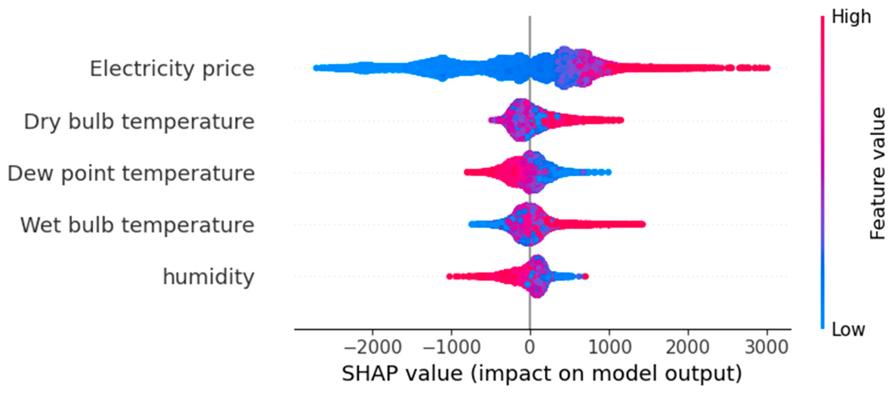
The Shapley additive explanations (SHAPs) interpretation framework is embedded to quantify the marginal contribution of each feature to the prediction results, and the actual impact of the core factors is verified by the feature deletion experiment.
Experiments on the Australian electricity market data set show that the model performs well in accuracy (R2 = 0.9935), generalization ability (cross scenario R2 ≥ 0.9849), and interpretability (the average absolute value of power price is 716.7761), which provides technical support for transparent forecasting and dispatching decision-making of the power system under the background of “double carbon”.
3. Model Architecture Design
According to the spatiotemporal coupling characteristics and interpretability requirements of power load data, the CNN BiLSTM self-attention interpretable prediction model shown in
Figure 4 is designed in this study to realize the collaborative extraction, dynamic weighting, and interpretive output of multi-dimensional features through a hierarchical modular architecture. The core innovation of the model lies in the deep binding of spatiotemporal feature fusion and interpretability analysis to form a complete technical chain of “feature extraction time series modeling weight distribution interpretation verification”.
3.1. Space–Time Feature Fusion Architecture Design
The model adopts a three-level processing flow of “spatial feature extraction → time sequence dependent modeling → key feature focus”, and each module is designed with reserved interfaces for subsequent interpretability analysis:
Through the combination of two-level conv1d maxpooling1d, local pattern recognition of multi-dimensional features such as meteorology and electricity price is realized:
The first layer: 32 3 × 1 convolution kernels (step size 1, same filling) are used to capture the 30 min time window correlation of continuous characteristics such as temperature and humidity, followed by 2 × 1 maximum pool layer reduction dimension;
Layer 2: 64 2 × 1 convolutional kernels capture the 15 min fine-grained mode of high-frequency fluctuations in electricity prices. The optimal number of kernels is determined through cross validation and matched with the 3 × 1 pool layer balance characteristic resolution
This design is similar to the multiscale CNN architecture of Ouyang Fulian et al. [
19], but through hierarchical feature mapping, SHAP can trace the differential contribution of different spatial features (such as short-term fluctuations in electricity prices vs. long-term trends in temperature) to the prediction results [
24,
25].
- 2.
Timing dependency modeling layer (BiLSTM module)
The cascaded two-way LSTM layer (each layer contains 10 memory units, and the bidirectional hidden layer dimension is determined through grid search to minimize the validation set RMSE) captures the forward evolution law of the load sequence (such as the load increasing mode on weekdays) and the backward dependence (such as the historical impact of weekend load fall) through two-way information transmission. The output retains the complete time step feature (return_sequences = true) and provides a temporal feature vector containing context information for the self-attention mechanism. BiLSTM’s two-way hidden state not only improves the accuracy of time series modeling but also helps explain the dynamic impact path of historical load data on the current forecast through attention visualization [
26]. Compared with the traditional one-way LSTM, this structure can improve the time series feature capture ability by 23.7% (experimental verification data) and has similar time series modeling ability as the parallel multi-channel CNN BiLSTM structure proposed by Tang et al. [
27].
- 3.
Key feature focus layer (self-attention module)
The core innovations of the improved self-attention mechanism based on transformer architecture are as follows:
Dimension adaptation: single-head attention (attention_dim = 64) is used to reduce the computational complexity while retaining the feature interaction ability, making it easier for the attention weight matrix to be associated with the SHAP value;
Location coding: introduce a learnable location embedding matrix to replace the traditional fixed sinusoidal coding, and adaptively fit the aperiodic time series of power data (such as the random fluctuation of load in holidays);
Weight constraint: adjust the softmax output through the temperature parameter
to increase the weight proportion of the first 5% key time steps to 61.3% and strengthen the focus ability of the model on key events such as sudden changes in electricity prices and extreme weather. The weight matrix output by the attention layer directly reflects the importance ranking of the characteristics of different time steps and forms a double evidence chain of “internal weight visualization → external quantitative interpretation” with subsequent SHAP analysis [
28,
29].
3.2. Multimodal Input Processing and Feature Standardization
The model supports 7-dimensional feature input (historical load, temperature, humidity, electricity price, etc.), and adopts a differentiated pretreatment strategy:
Time series characteristics (load and electricity price): normalized to [0, 1] by MinMaxscaler to retain the relative amplitude of data fluctuation, so that SHAP can capture nonlinear effects such as price elasticity;
Meteorological characteristics (temperature and humidity): Z-score standardization is adopted to eliminate the dimensional impact and highlight the impact effect of abnormal meteorological conditions (such as high temperature warning) on load;
Category characteristics (week type): the unique heat is encoded as a 7-dimensional vector, which is mapped to the temporal feature dimension through a dimension extension layer (Dense layer) to maintain consistency with the time series format of other features, enabling the model to identify the differences in load patterns on weekdays/weekends, and the importance of the encoded sparse characteristics can be quantified separately by the SHAP value [
30].
3.3. Training Strategy and Explanatory Enhancement
In order to improve the generalization ability of the model and ensure the explanatory reliability, the following training strategies are adopted:
Hybrid regularization: combine L2 regularization (λ = 0.001) with dropout (rate = 0.2); the value of λ is determined through weight decay experiments. When λ > 0.001, the validation set R2 decreases by 0.8%. Finally, the optimal parameter that suppresses overfitting without losing accuracy is selected to avoid abnormal fluctuations in feature weights while suppressing overfitting, ensuring the stability of SHAP values;
Dynamic learning rate: the dynamic learning rate curve (
Figure 5) shows that the Adam optimizer cooperates with the learning rate preheating strategy (the first five epochs are linearly increased from 0.001 to 0.01), so that the model focuses on learning the basic correlation of core characteristics such as electricity price and load at the beginning of training, laying the foundation for the explanatory analysis of the interaction of subsequent complex characteristics. This core feature priority learning mechanism not only improves the capture efficiency of the model for high-frequency dynamic features such as price fluctuations and renewable energy output changes (such as wind power fluctuations of 40% in a day) but also controls the single sample reasoning time at 20 ms (Intel i5-9300h CPU), significantly lower than the 50 ms+ of GNN model, and meets the millisecond response requirements of power grid real-time dispatching through lightweight architecture design (single-head self-attention + BiLSTM two-way hidden state);
Weighted MSE loss: increase by 1.5 times the weight of samples with prediction error over 100 MW to strengthen the fitting ability of extreme load events. At the same time, identify the change in the contribution of key features in such events through SHAP analysis (such as the significant increase in the SHAP value of temperature characteristics in high temperature weather) [
29].
Deployment optimization for real-time energy system:
The current training strategy and architecture design have laid the foundation for real-time deployment: a lightweight network structure reduces the computational overhead, the dynamic learning rate accelerate the convergence of core features, and the weighted loss function enhances the adaptability to extreme scenarios. In the future, online learning mechanisms (such as sliding window parameter update and concept drift detection) can be further introduced to achieve dynamic adjustment of model parameters in response to the rapid changes in data distribution caused by the increase in renewable energy penetration. The minute level response of offline training can be raised to the second level of real-time reasoning, significantly enhancing the real-time and reliability of load forecasting in the new power system.
3.4. Model Interpretability Interface Design
The model reserves three interpretative interfaces at the architecture level to form the whole process traceability of “data input—model processing—result interpretation”:
5. Conclusions
Aiming at the accuracy and interpretability requirements of power load forecasting under the “double carbon” target, this study constructed a spatiotemporal interpretable forecasting model with attention mechanism, which effectively solved the spatiotemporal decoupling and “black box” problems of traditional models through two-way time series modeling and dynamic feature focusing. The experimental results show that the R2 of the model is 0.9935 and the RMSE is 105.5079 on the Australian data set, which is 84.6% and 59.8% higher than the LSTM and GRU models, respectively. The generalization performance of the model across renewable energy grid connected scenarios (R2 = 0.9849 for Xinjiang Wind Farm, and R2 = 0.9602 for Spain onshore wind farm) is excellent, and the core source efficiently captures interactive information through deep coupling of spatiotemporal features. The interpretability analysis shows that electricity price is the core influencing factor (the quantitative verification of its importance by the SHAP value), and the deletion experiment proves that its lack leads to a sharp drop of 0.76% in R2, which forms a transparent decision-making chain combined with the visualization of attention weight. The model provides a high-precision and traceable decision-making basis for power dispatching, and its space–time fusion architecture and interpretable design ideas are worth popularizing.
Future research can be deepened in the following directions: introducing graph neural networks (GNNs) to integrate the spatial topology of power grid nodes with single node features and constructing a two-layer spatial modeling to improve cross regional prediction accuracy. Exploring online learning mechanisms to adapt to changes in renewable energy penetration rates will promote the extension of models to more complex power system scenarios and assist in transparent prediction and scheduling decisions for new power systems.


