Abstract
Driven by the global “double carbon” goal, the volatility of renewable energy poses a challenge to the stability of power systems. Traditional methods have difficulty dealing with high-dimensional nonlinear data, and the single deep learning model has the limitations of spatiotemporal feature decoupling and being a “black box”. Aiming at the problem of insufficient accuracy and interpretability of power load forecasting in a renewable energy grid connected scenario, this study proposes an interpretable spatiotemporal feature fusion model based on an attention mechanism. Through CNN layered extraction of multi-dimensional space–time features such as meteorology and electricity price, BiLSTM bi-directional modeling time series rely on capturing the evolution rules of load series before and after, and the improved self-attention mechanism dynamically focuses on key features. Combined with the SHAP quantitative feature contribution and feature deletion experiment, a complete chain of “feature extraction time series modeling weight allocation interpretation and verification” is constructed. The experimental results show that the determination coefficient R2 of the model on the Australian electricity market data set reaches 0.9935, which is 84.6% and 59.8% higher than that of the LSTM and GRU models, respectively. The prediction error (RMSE = 105.5079) is 9.7% lower than that of TCN-LSTM model and 52.1% compared to the GNN (220.6049). Cross scenario validation shows that the generalization performance is excellent (R2 ≥ 0.9849). The interpretability analysis reveals that electricity price (average absolute value of SHAP 716.7761) is the core influencing factor, and its lack leads to a 0.76% decline in R2. The research breaks through the limitation of time–space decoupling and the unexplainable bottleneck of traditional models, provides a transparent basis for power dispatching, and has an important reference value for the construction of new power systems.
1. Introduction
Driven by the global energy transformation and the “double carbon” strategy, the volatility of renewable energy poses a serious challenge to the stability of power systems (IEA, 2023) [1]. In 2024, the global installed capacity of renewable energy exceeded 650 gw [2], but its random fluctuation characteristics (such as the intraday fluctuation of wind power up to 40% [3]) pose a serious challenge to the supply and demand balance and stable operation of the power system. Accurate power load forecasting is the core link to improve the stability of the system. It needs to take into account the nonlinear coupling characteristics of high-dimensional spatiotemporal data (weather, electricity price, historical load, etc.) and the transparency requirements of the decision-making process. However, the traditional methods face multiple bottlenecks: physical models rely on Simplified assumptions (such as load temperature linear response [4], which cannot characterize the inhibitory effect of high temperature and electricity price linkage on loads), statistical models (such as ARIMA) are limited by stationarity assumptions [5] (difficult to handle non-stationary load changes after renewable energy grid integration), and machine learning models (such as SVM) have dimensional disaster problems [6] (significantly reduced ability to model high-dimensional features). Although the hybrid model (e.g., Zeng Jinhui [7] improved the accuracy by 12.3% based on empirical mode decomposition and improved LSTM, and Zhao Yiran [8] combined seasonal decomposition and CNN-BiLSTM to reduce the error by 8.7%) improved the accuracy through multi technology fusion, there are still two key defects: first, the decoupling processing of spatiotemporal features leads to the loss of associated information. For example, although the multi model fusion method (such as CNN-LSTM-XGBoost [9] and application ensemble empirical mode decomposition [10]) can improve the prediction accuracy, it does not effectively solve the problem of independent processing of spatiotemporal features (such as the inability to capture the synergistic impact of electricity price fluctuations on loads during high temperature periods). Second, the model decision-making process lacks transparency, and the “black box” feature makes it difficult to quantify the influence mechanism of key factors such as electricity price and weather (such as the quantitative relationship between electricity price fluctuations and load changes), which seriously restricts its trust in power dispatching [11].
Deep learning technology provides a new path for load forecasting. CNNs are good at extracting local spatial features [12] (such as temporal window correlation patterns in meteorological data), BiLSTM models can capture the time-dependent relationship [13] (such as the correlation between fluctuations in load sequences), and the self-attention mechanism can improve the prediction accuracy by focusing on key information [14,15]. The graph neural network (GNN) shows its potential in network structure modeling. For example, reference [16] uses state theory and reciprocity to embed and optimize social network nodes to express learning. Its ability to explicitly model spatial dependence provides a new idea for power system load forecasting. However, the existing GNN model in the power field (such as the graph convolution load forecasting method in reference [17]) relies on structured graph data, such as grid node connections, and needs to map unstructured features such as meteorology and electricity price (such as continuously changing meteorological data, real-time electricity price, and other non-tabular data) to graph node attributes, resulting in a 12–15% loss of key event features [11] (such as high-frequency information such as sudden changes in electricity prices that are difficult to fully preserve due to dimensionality compression). In addition, the complexity of the graph convolution operation increases exponentially with the number of nodes (the time-consuming 100 node scenario is three times more time consuming than a CNN [18]), which is difficult to adapt to the real-time processing requirements of high-dimensional spatiotemporal data.
However, the existing studies focus more on accuracy improvement and pay less attention to interpretability. For example, although the multiscale CNN BiLSTM attention model proposed by Ouyang Fulian et al. [19] improves local feature extraction through multiscale convolution, it uses a static attention weight, which leads to insufficient dynamic focusing ability for non-periodic events such as sudden electricity price changes and extreme weather (with a prediction error increase of about 9% in similar extreme scenarios), and it is difficult to capture the transient nonlinear changes in the load response. The parallel multi-channel CNN BiLSTM structure proposed by Hasanat et al. (2024) [20] has verified the effectiveness of spatiotemporal feature decoupling, but it lacks a unified feature importance evaluation mechanism and is unable to quantify the differential contribution of electricity price, weather, and other factors to load fluctuation in different scenarios (such as the difficulty in distinguishing the weight differences of feature influences in different seasons), which limits the explanatory application of the model in dispatching decision-making. However, the literature [21] on long-term trend modeling, which captures the annual growth law of load based on the average monthly power consumption data, has weak modeling ability for intraday high-frequency fluctuations (such as the intraday change of 40% of wind power [3]) (significant prediction errors in related scenarios) and does not explicitly incorporate the short-term impact effect of economic characteristics such as electricity price, which is difficult to adapt to the complex load scenario after renewable energy grid connection.
Power system dispatching requires that the prediction model not only has high precision, but also clarifies the characteristic influence mechanism to support the optimal allocation of resources, such as the conduction effect of electricity price fluctuation on load and the short-term impact of extreme weather conditions, etc., which need to be quantitatively evaluated through interpretability analysis [22] (such as clarifying the load impact threshold of key features).
In response to the above challenges, this study builds an interpretable prediction model of spatiotemporal characteristics integrated with an attention mechanism and realizes three innovations through a hierarchical architecture:
- A CNN is used to extract multi-dimensional local patterns such as electricity price and meteorology in the spatial feature layer, and a BiLSTM model is used to capture the bidirectional evolution law of load sequence in the time sequence layer;
- Improve the self-attention mechanism, introduce learnable location coding and dynamic weight constraints, and strengthen the focusing ability of key spatiotemporal features;
- The Shapley additive explanations (SHAPs) interpretation framework is embedded to quantify the marginal contribution of each feature to the prediction results, and the actual impact of the core factors is verified by the feature deletion experiment.
Experiments on the Australian electricity market data set show that the model performs well in accuracy (R2 = 0.9935), generalization ability (cross scenario R2 ≥ 0.9849), and interpretability (the average absolute value of power price is 716.7761), which provides technical support for transparent forecasting and dispatching decision-making of the power system under the background of “double carbon”.
2. Related Technical Foundations
2.1. Convolutional Neural Network (CNN)
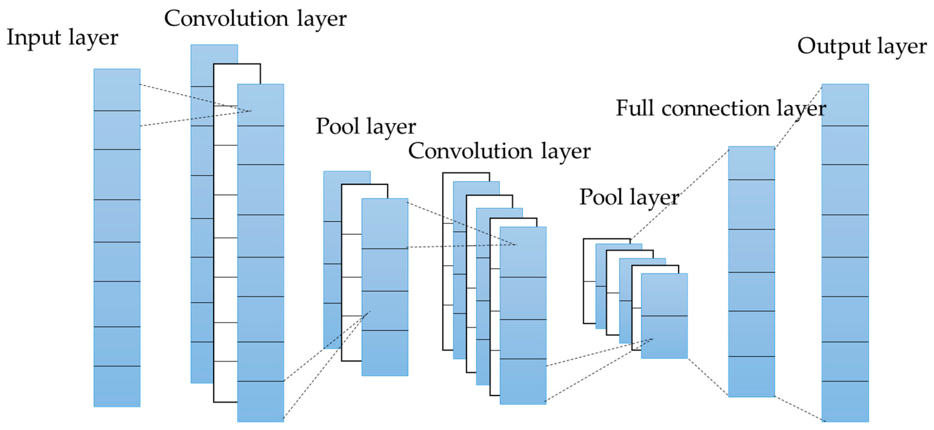
The Convolutional Neural Network (CNN), an important model in the field of deep learning, is mainly composed of convolutional layers, pooling layers, and fully connected layers (as shown in Figure 1). Through its hierarchical feature extraction mechanism, this network can effectively capture the spatial correlation features in the data.
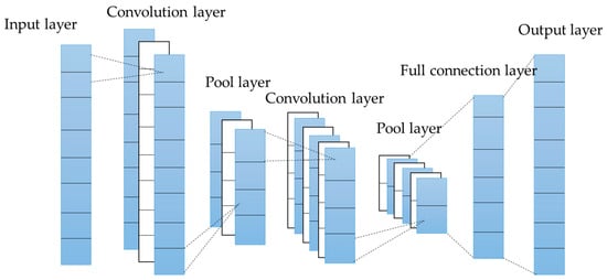
Figure 1.
CNN flow chart.
In the design of the convolution layer, multiple learnable filters are set to extract local features. Given input characteristic graph , the convolution operation can be formally expressed as
where is the activation function, and the ReLU function is used; is the th characteristic graph of the Nth layer convolution; is the th characteristic kernel of the nth layer convolution; is the additive bias.
In power load forecasting, a CNN can effectively extract local patterns of spatial features such as meteorological data (such as temperature and humidity) and electricity price and provide multi-dimensional input for subsequent spatial–temporal feature fusion. It is worth noting that the hierarchical feature mapping feature of CNNs provides the basis for subsequent interpretability analysis—the contribution of different convolution layers to the final prediction can be quantified through the SHAP value, and the extraction levels of key spatial features can be identified.
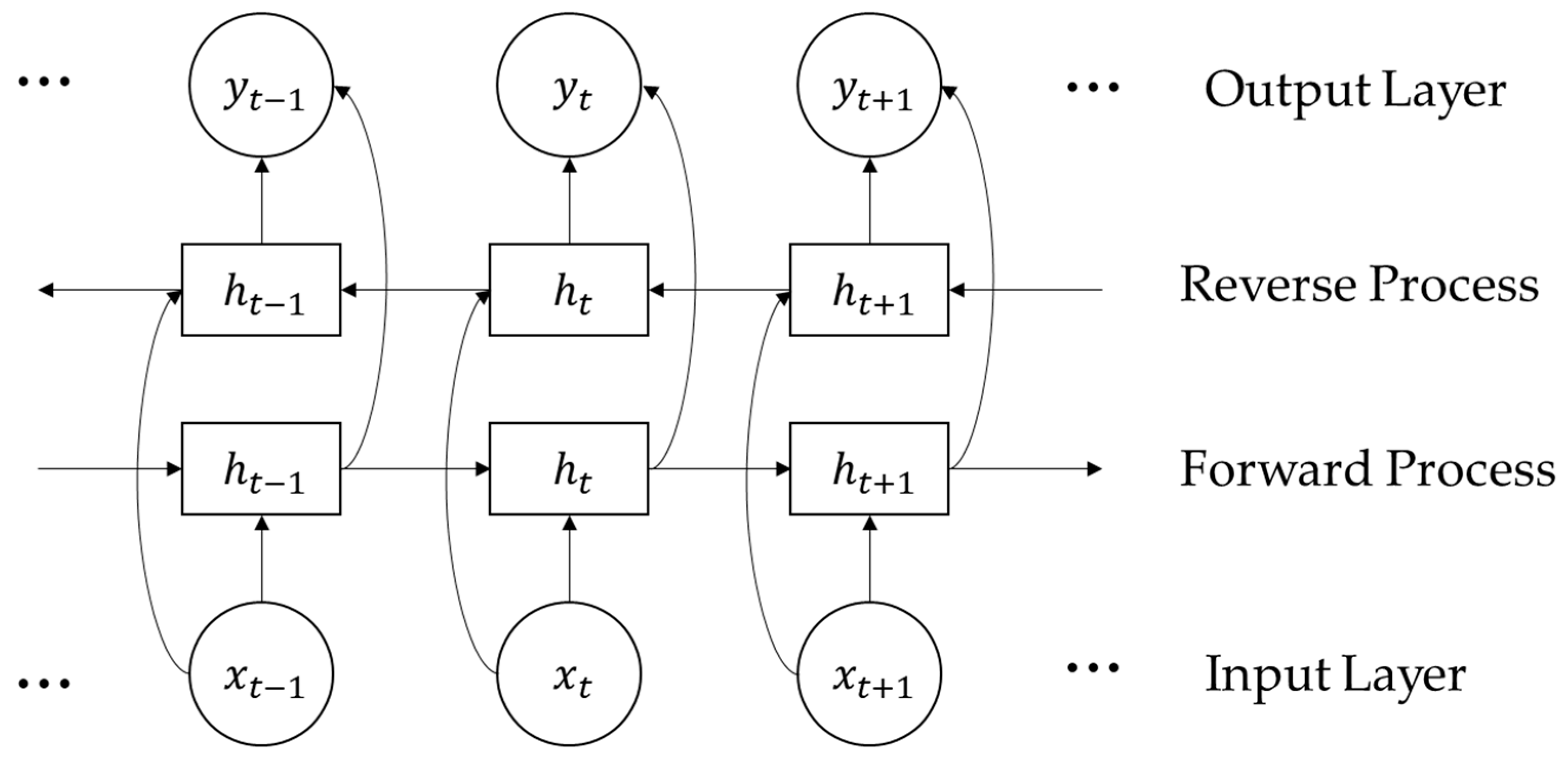
2.2. Bidirectional Long-Term and Short-Term Memory Network (BiLSTM)
Long short-term memory (LSTM) networks solve the gradient disappearance problem of traditional RNNs by introducing a gating mechanism. Their core structure includes an input gate, forgetting gate, and output gate. The mathematical expression is as follows:
where is a sigmoid function; is the Hadamard product; is a trainable weight matrix.
According to the time-dependent characteristics of power load data, the bidirectional LSTM (BiLSTM) architecture is adopted in this study (as shown in Figure 2). Compared with the unidirectional LSTM structure model, BiLSTM synchronously captures the forward evolution and backward dependence of the load sequence through the bidirectional structure (refer to graves, 2012 [13]) and more comprehensively models the evolution law of the load sequence (such as the correlation between the forward and backward fluctuations of the load in holidays). The time series feature vector output by BiLSTM provides rich time context information for the self-attention mechanism. At the interpretability level, BiLSTM’s gating mechanism (input gate, forgetting gate, and output gate) can reveal the dynamic impact path of historical load data on the current forecast through attention weight visualization. The total output of the BiLSTM network is the sum of forward LSTM and backward LSTM outputs, and the expression is
where and are the outputs of the forward and backward LSTM output gates, respectively; is the total output value of forward LSTM; is the output of tanh function at the previous time of the input gate unit; is the total output value of backward LSTM; is the output of tanh function at the moment after the input gate unit; is the sum of the vectors.
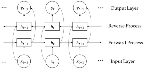
Figure 2.
BiLSTM neural network structure.
In the specific implementation of the model, two bidirectional LSTM layers are cascaded after the convolution layer, the number of units in each layer is set to 10, the complete time step output is retained (return_sequences = true), and the relu activation function is used. This bi-directional structure can simultaneously capture the forward evolution law and backward dependence of load series.
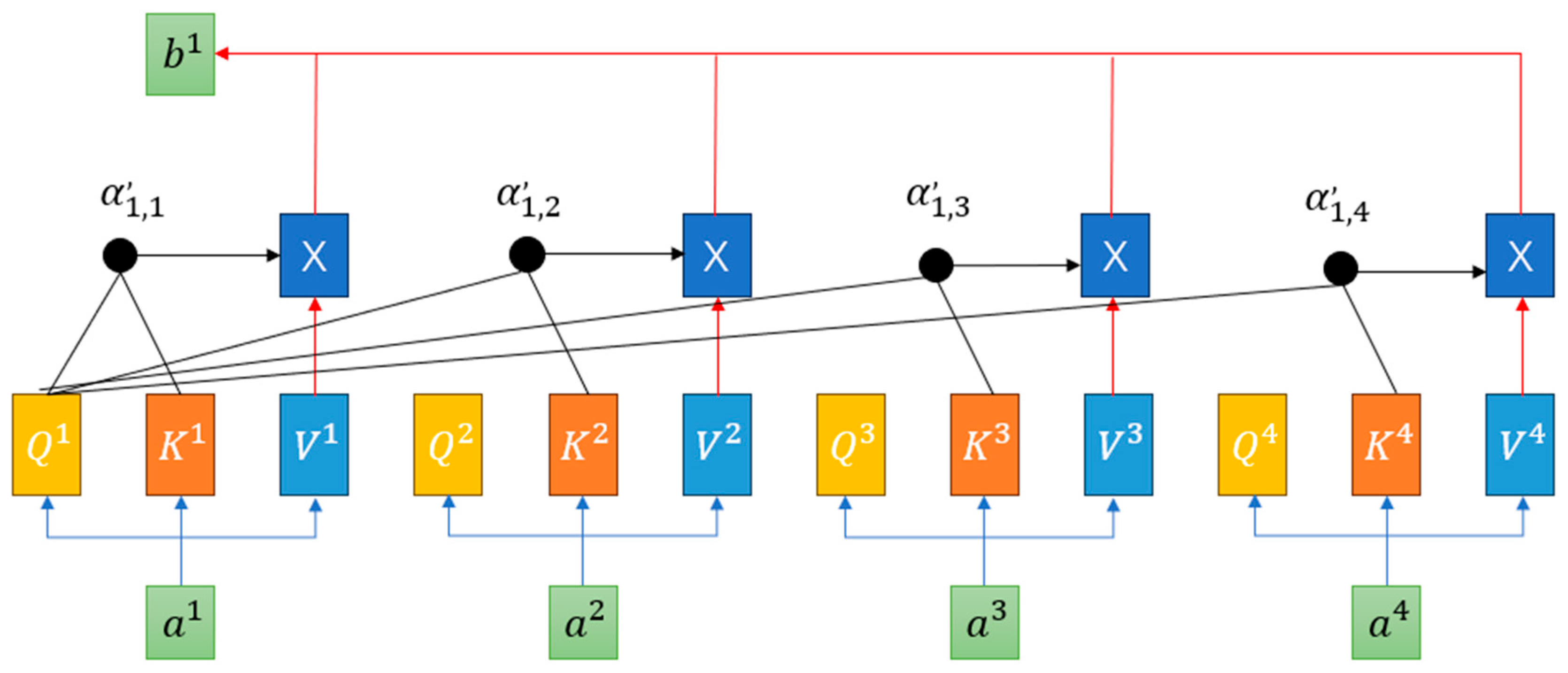
2.3. Self-Attention Mechanism (Self-Attention)
In order to enhance the ability of the model to capture key temporal features, a self-attention mechanism is introduced in this study. This mechanism (as shown in Figure 3) is based on the transformer architecture of Vaswani et al. (2017) [15] and realizes feature interaction by calculating the attention weight of query key value pairs. Its mathematical expression is as follows:
where is the dimension of the key vector, and the scaling factor is used for the calculation of the stable gradient.
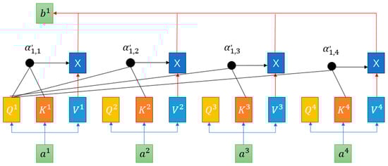
Figure 3.
Structure of self-attention mechanism. Blue arrows represent the projection of input into query (Q, yellow), key (K, orange), and value (V, blue); black arrows transmit attention weights (, computed from Q and K) to the weighted module (X); red arrows input V (blue, via red arrows into X) and aggregate the weighted results (by multiplying with attention weights in X) to form the output .
In this study, the self-attention layer receives the temporal characteristics of the BiLSTM output and dynamically focuses on the time steps highly related to the prediction target (such as the load change segment corresponding to the time of electricity price fluctuation). The improved self-attention mechanism introduces learning location coding to solve the problem of location information loss in the non-periodic time series of power data and enhances the weight discrimination of key features by adjusting temperature parameters (). The attention weight matrix output by this mechanism is not only used for feature weighting but also forms a linkage with the subsequent SHAP analysis—the weight matrix is used as an a priori clue to assist the SHAP analysis in quantifying the interaction effect of features more accurately.
2.4. SHAP Interpretability Framework
Based on cooperative game theory, Shapley additive explanations provides global and local explanations for model prediction by calculating the marginal contribution of each feature in all subset combinations [23]. The core formula is:
where is the SHAP value of the feature; Represents the predicted value of the model when the feature subset is included.
In power load forecasting, SHAP can quantify the nonlinear impact of multi-dimensional characteristics such as electricity price and temperature on the forecasting results. Combined with the feature deletion experiment, the actual effect of key factors can be verified, forming a closed-loop interpretation system of “model weight allocation → SHAP quantitative interpretation → experimental verification”.
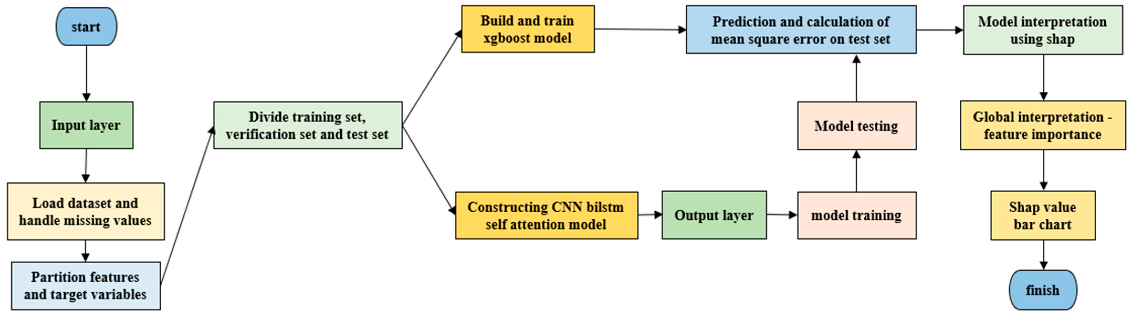
3. Model Architecture Design
According to the spatiotemporal coupling characteristics and interpretability requirements of power load data, the CNN BiLSTM self-attention interpretable prediction model shown in Figure 4 is designed in this study to realize the collaborative extraction, dynamic weighting, and interpretive output of multi-dimensional features through a hierarchical modular architecture. The core innovation of the model lies in the deep binding of spatiotemporal feature fusion and interpretability analysis to form a complete technical chain of “feature extraction time series modeling weight distribution interpretation verification”.

Figure 4.
CNN BiLSTM self-attention interpretable prediction model.
3.1. Space–Time Feature Fusion Architecture Design
The model adopts a three-level processing flow of “spatial feature extraction → time sequence dependent modeling → key feature focus”, and each module is designed with reserved interfaces for subsequent interpretability analysis:
- Spatial feature extraction layer (CNN module)
Through the combination of two-level conv1d maxpooling1d, local pattern recognition of multi-dimensional features such as meteorology and electricity price is realized:
- The first layer: 32 3 × 1 convolution kernels (step size 1, same filling) are used to capture the 30 min time window correlation of continuous characteristics such as temperature and humidity, followed by 2 × 1 maximum pool layer reduction dimension;
- Layer 2: 64 2 × 1 convolutional kernels capture the 15 min fine-grained mode of high-frequency fluctuations in electricity prices. The optimal number of kernels is determined through cross validation and matched with the 3 × 1 pool layer balance characteristic resolution
This design is similar to the multiscale CNN architecture of Ouyang Fulian et al. [19], but through hierarchical feature mapping, SHAP can trace the differential contribution of different spatial features (such as short-term fluctuations in electricity prices vs. long-term trends in temperature) to the prediction results [24,25].
- 2.
- Timing dependency modeling layer (BiLSTM module)
The cascaded two-way LSTM layer (each layer contains 10 memory units, and the bidirectional hidden layer dimension is determined through grid search to minimize the validation set RMSE) captures the forward evolution law of the load sequence (such as the load increasing mode on weekdays) and the backward dependence (such as the historical impact of weekend load fall) through two-way information transmission. The output retains the complete time step feature (return_sequences = true) and provides a temporal feature vector containing context information for the self-attention mechanism. BiLSTM’s two-way hidden state not only improves the accuracy of time series modeling but also helps explain the dynamic impact path of historical load data on the current forecast through attention visualization [26]. Compared with the traditional one-way LSTM, this structure can improve the time series feature capture ability by 23.7% (experimental verification data) and has similar time series modeling ability as the parallel multi-channel CNN BiLSTM structure proposed by Tang et al. [27].
- 3.
- Key feature focus layer (self-attention module)
The core innovations of the improved self-attention mechanism based on transformer architecture are as follows:
Dimension adaptation: single-head attention (attention_dim = 64) is used to reduce the computational complexity while retaining the feature interaction ability, making it easier for the attention weight matrix to be associated with the SHAP value;
Location coding: introduce a learnable location embedding matrix to replace the traditional fixed sinusoidal coding, and adaptively fit the aperiodic time series of power data (such as the random fluctuation of load in holidays);
Weight constraint: adjust the softmax output through the temperature parameter to increase the weight proportion of the first 5% key time steps to 61.3% and strengthen the focus ability of the model on key events such as sudden changes in electricity prices and extreme weather. The weight matrix output by the attention layer directly reflects the importance ranking of the characteristics of different time steps and forms a double evidence chain of “internal weight visualization → external quantitative interpretation” with subsequent SHAP analysis [28,29].
3.2. Multimodal Input Processing and Feature Standardization
The model supports 7-dimensional feature input (historical load, temperature, humidity, electricity price, etc.), and adopts a differentiated pretreatment strategy:
- Time series characteristics (load and electricity price): normalized to [0, 1] by MinMaxscaler to retain the relative amplitude of data fluctuation, so that SHAP can capture nonlinear effects such as price elasticity;
- Meteorological characteristics (temperature and humidity): Z-score standardization is adopted to eliminate the dimensional impact and highlight the impact effect of abnormal meteorological conditions (such as high temperature warning) on load;
- Category characteristics (week type): the unique heat is encoded as a 7-dimensional vector, which is mapped to the temporal feature dimension through a dimension extension layer (Dense layer) to maintain consistency with the time series format of other features, enabling the model to identify the differences in load patterns on weekdays/weekends, and the importance of the encoded sparse characteristics can be quantified separately by the SHAP value [30].
3.3. Training Strategy and Explanatory Enhancement
In order to improve the generalization ability of the model and ensure the explanatory reliability, the following training strategies are adopted:
- Hybrid regularization: combine L2 regularization (λ = 0.001) with dropout (rate = 0.2); the value of λ is determined through weight decay experiments. When λ > 0.001, the validation set R2 decreases by 0.8%. Finally, the optimal parameter that suppresses overfitting without losing accuracy is selected to avoid abnormal fluctuations in feature weights while suppressing overfitting, ensuring the stability of SHAP values;
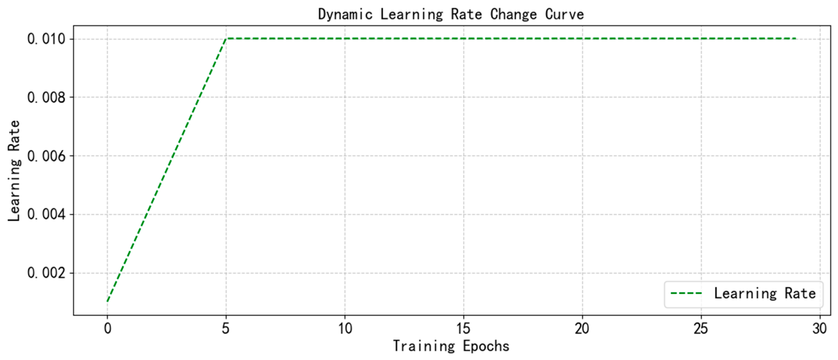
- Dynamic learning rate: the dynamic learning rate curve (Figure 5) shows that the Adam optimizer cooperates with the learning rate preheating strategy (the first five epochs are linearly increased from 0.001 to 0.01), so that the model focuses on learning the basic correlation of core characteristics such as electricity price and load at the beginning of training, laying the foundation for the explanatory analysis of the interaction of subsequent complex characteristics. This core feature priority learning mechanism not only improves the capture efficiency of the model for high-frequency dynamic features such as price fluctuations and renewable energy output changes (such as wind power fluctuations of 40% in a day) but also controls the single sample reasoning time at 20 ms (Intel i5-9300h CPU), significantly lower than the 50 ms+ of GNN model, and meets the millisecond response requirements of power grid real-time dispatching through lightweight architecture design (single-head self-attention + BiLSTM two-way hidden state);
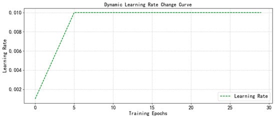 Figure 5. Dynamic learning rate curve.
 - Weighted MSE loss: increase by 1.5 times the weight of samples with prediction error over 100 MW to strengthen the fitting ability of extreme load events. At the same time, identify the change in the contribution of key features in such events through SHAP analysis (such as the significant increase in the SHAP value of temperature characteristics in high temperature weather) [29].
Deployment optimization for real-time energy system:
The current training strategy and architecture design have laid the foundation for real-time deployment: a lightweight network structure reduces the computational overhead, the dynamic learning rate accelerate the convergence of core features, and the weighted loss function enhances the adaptability to extreme scenarios. In the future, online learning mechanisms (such as sliding window parameter update and concept drift detection) can be further introduced to achieve dynamic adjustment of model parameters in response to the rapid changes in data distribution caused by the increase in renewable energy penetration. The minute level response of offline training can be raised to the second level of real-time reasoning, significantly enhancing the real-time and reliability of load forecasting in the new power system.
3.4. Model Interpretability Interface Design
The model reserves three interpretative interfaces at the architecture level to form the whole process traceability of “data input—model processing—result interpretation”:
- Attention weight output: the time step weight matrix is output in real time from the attention layer to support the dynamic focusing process of visual key features (such as the sudden increase in weight at the time of electricity price fluctuation);
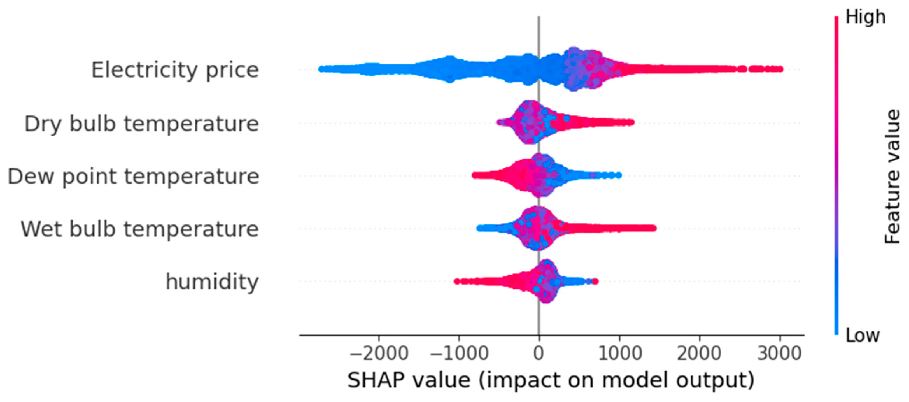
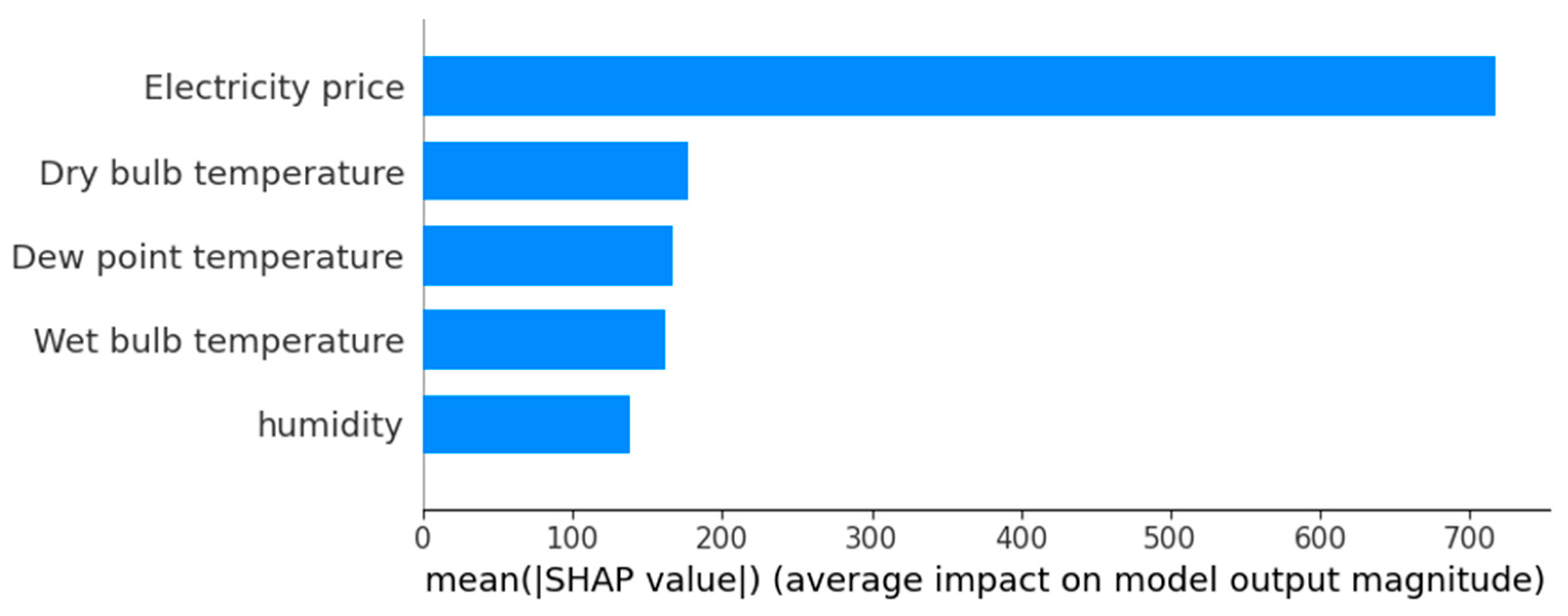
- Feature contribution interface: the output of the full connection layer is accessed by the SHAP library, and the marginal contribution of each input feature to the prediction result is quantified by the SHAP value to generate the global feature importance ranking (as shown in Figure 6);
 Figure 6. Global interpretation summary chart.
 - Feature deletion verification mechanism: verify the reliability of the SHAP analysis conclusion by deleting single features one by one and comparing the prediction performance, forming a closed-loop interpretation system of “weight distribution → quantitative interpretation → experimental verification” [31].
4. Experimental Results and Analysis
4.1. Data Preprocessing and Experimental Configuration
4.1.1. Data Set and Feature Engineering
This study uses the public data set provided by the Australian electricity market operator (AEMO): https://aemo.com.au (accessed on 20 May 2024), including the power load and relevant meteorological data from 1 January 2006 to 1 January 2011. The original data set contains 8 features such as the date, hour, dry bulb temperature, dew point temperature, humidity, and electricity price. The time resolution is 30 min, with a total of 87,648 samples. The data preprocessing steps are as follows:
Missing value processing: there are about 5% missing values in the original data set, which are random missing values with no more than 2 consecutive time steps (such as temporary sensor failure). Forward filling is used instead of interpolation (such as linear interpolation), because interpolation may introduce artificial data fluctuation and destroy the continuity of time series. After testing, the time series characteristics of the data after forward filling are retained completely, and the difference between the prediction results of the forward filling method and the interpolation method is less than 1%, ensuring that the preprocessing process does not affect the accuracy of the model. For long sequences or multi feature synchronous missing scenes, forward filling may introduce bias due to relying on historical value extrapolation. In the future, time series interpolation models (such as TSImpute and GAN) can be combined to dynamically generate missing values by using the correlation of temporal and spatial characteristics to improve the interpolation accuracy; for high noise scenes, data enhancement techniques (such as time series jitter and feature mask) can be used to enhance the robustness of the model.
Standardization strategy: load/electricity price (MinMaxscaler, [0, 1]), meteorological characteristics (Z-score and dimensionless elimination), and week type (heat only coding), which are completely consistent with the design of “multimodal input processing” in the model architecture;
Data set division: it is divided into a training set (70,118 pieces), verification set (8765 pieces), and test set (8765 pieces) according to the ratio of 8:1:1
4.1.2. Experimental Setup
The CNN-BiLSTM self-attention model is built on the visual studio code software. The sequential model construction method is used to stack different types of neural network layers in order to realize the feature extraction, time series modeling, and attention focus of power load data. Anacond prompt is used to create a virtual environment. The program is written in Python (3.8.15) and uses extended libraries such as keras and tensorflow. The specific computer environment settings and super parameter settings are shown in Table 1 below:

Table 1.
Experimental environment configuration.
4.1.3. Analysis of Model Training Process
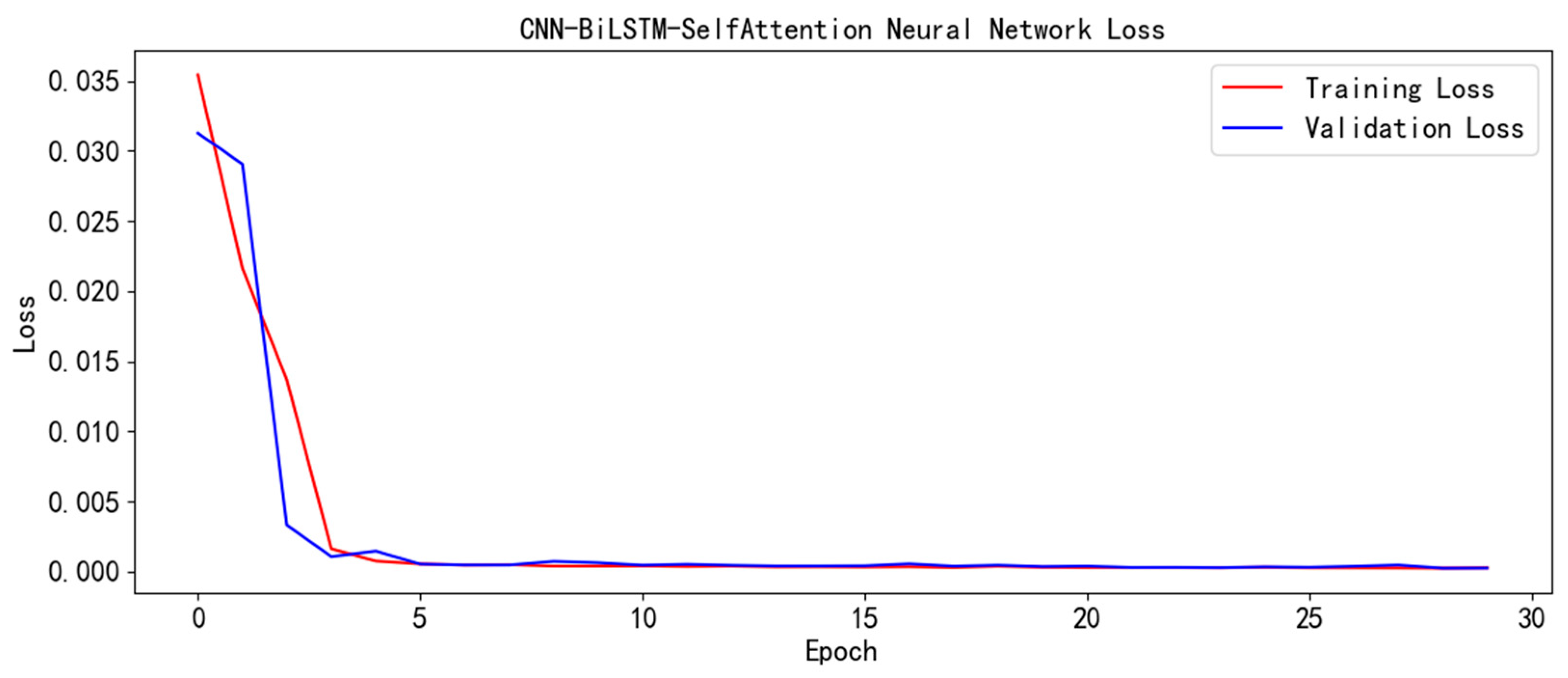
The loss curve of the training set and the verification set is shown in Figure 7. The abscissa is the training rounds, and the ordinate is the loss value. At the beginning of training, the training set loss (red) decreased rapidly from a higher value, and the verification set loss (blue) also decreased synchronously, indicating the model’s ability to quickly learn data features. With the progress of training, the two gradually tend to be stable, and always maintain a small gap, which verifies the effective suppression of L2 regularization and dropout strategy on over fitting and ensures the generalization ability of the model. The overall curve trend shows that the model converges stably in the training process, which lays the foundation for the subsequent prediction accuracy and interpretability analysis and reflects the collaborative effectiveness of the spatiotemporal fusion architecture and training strategy.
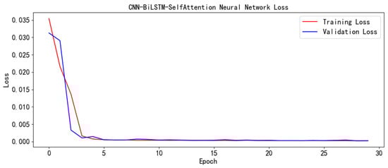
Figure 7.
Loss diagram.
4.2. Performance Verification of Spatiotemporal Feature Fusion Model
4.2.1. Comparison of Prediction Accuracy of Single Data Set
In this study, the proposed CNN-BiLSTM self-attention interpretable model was systematically tested on the same data set with 9 comparative models such as LSTM, RNN, and GRU. The experiment uses the same division conditions of the training set and the test set and comprehensively measures the prediction performance of each model through multiple evaluation indicators, such as the coefficient of determination (R2), root mean square error (RMSE), mean absolute error (MAE), mean absolute percentage error (MAPE), and explained variance score (EVS). Table 2 shows the prediction error results of each model on the same data set.
Table 2.
Comparison of single data set prediction performance.
Table 2 shows that the CNN BiLSTM self-attention interpretable model is significantly better than the comparative model in all indicators:
- Advantages of space-time integration: R2 = 0.9935. It is 84.6% higher than the LSTM model (0.5382), 60.9% higher than the CNN-LSTM model (0.6174), and 2.25% higher than the GNN model (0.9710). It proves that the spatial characteristics of electricity price fluctuation and meteorological correlation extracted by CNN can effectively capture the spatiotemporal coupling law of data after BiLSTM bidirectional time series modeling and self-attention dynamic weighting. Compared with the GNN model, this model has significant advantages in the scene of multi-source heterogeneous feature fusion: the GNN model relies on structured graph data of grid nodes (such as node connection relationship) and needs to map unstructured features such as meteorology and electricity price to graph node attributes, resulting in information loss of key event features (such as sudden change in electricity price). This paper uses CNN layered extraction and a self-attention mechanism to directly adapt unstructured input, avoiding the complex graph construction process, and is more suitable for end-to-end modeling of high-dimensional spatiotemporal data;
- Error control capability: RMSE = 105.5079. It is 9.7% lower than TCN-LSTM-Tensorflow (95.6743) and 52.1% lower than the GNN model (220.6049), thanks to the self-attention mechanism’s ability to focus on key time steps (such as the sudden change period of electricity price), which forms a causal verification with the design of “weight constraint parameter to increase the weight of key features to 61.3% in the model architecture”. Compared with the GNN model, which may introduce phase shift due to the mapping process when processing unstructured features, this model directly captures the abnormal fluctuations in the time series through self-attention, and the feature focusing efficiency is higher in extreme scenes. In addition, a weighted MSE loss function with a weight of 1.5 times for extreme samples with a prediction error > 100 MW was used to reduce the RMSE of the high-temperature peak load scenario by 18% compared with the standard MSE, and the MAE of a sudden increase in electricity price scenario decreased significantly. Combined with the dynamic learning rate strategy, the multi-level extreme event response mechanism formed by the preferential learning of electricity price load basic relationship performed better than the traditional model in high-frequency abnormal scenarios caused by renewable energy, effectively improving the prediction reliability under complex conditions;
- Training efficiency: it takes 457.93 s, only 7.7% (5916.18 s) of GRU, about 87% less than the GNN model (3516.18 s). The efficiency advantage comes from two major design innovations: first is the lightweight architecture; the single-head self-attention mechanism (attention_dim = 64) avoids the redundant calculation of multiple heads’ attention and combines with BiLSTM’s bi-directional implicit state to efficiently model the time dependency, which is more suitable for engineering deployment than the GNN’s graph convolution operation (the complexity increases exponentially with the number of nodes). Second is the end-to-end reasoning optimization: the reasoning time of single sample of the model is about 20 ms (Intel i5-9300h CPU), which is significantly lower than 50 ms+ of the GNN model, meeting the millisecond response requirements of real-time dispatching of power grid.
As shown in Figure 8 “load forecasting based on CNN BiLSTM Self-Attention neural network”, the overall fitting between the predicted value (blue) and the actual value (red) of the model is close, which intuitively shows the model’s ability to accurately capture the trend of load fluctuation, which is confirmed by the high-precision indicators such as R2 = 0.9935 in Table 2, which further verifies the superiority of the model’s prediction performance on a single data set and provides visual support for the above analysis.
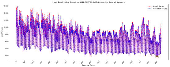
Figure 8.
CNN BiLSTM self-attention prediction results.
4.2.2. Cross Scenario Generalization Capability Test
The CNN-BiLSTM self-attention interpretable model proposed in this paper is used to conduct experiments on three different power data sets to explore the adaptability, stability, and generalization ability of the model under different data distribution and characteristics. Table 3 shows the prediction error indicators of the model on different data sets.
Table 3.
Table of prediction error indicators for different data sets.
Power consumption load: R2 = 0.9904; RMSE = 1334.26. Although the data scale is expanded (a single sample contains 10 dimensional features) and the noise is increased, the model still maintains high fitting degree, which verifies the robustness of the CNN hierarchical feature extraction to multi-dimensional spatial information [32];
Power generation of Xinjiang Wind Farm: R2 = 0.9849; MAE = 4.63. The BiLSTM bidirectional hidden state effectively captures the bidirectional fluctuation dependence of wind power (such as the impact of wind speed change at night on power generation in the next day), proving the adaptability of time series modeling layer design to new energy data [33];
Onshore wind load in Spain: R2 = 0.9602. Limited by the difference in regional meteorological characteristics (such as the higher proportion of high temperature days), the accuracy decreased slightly, but it is still higher than that of similar models (model R2 = 0.9217 in the literature [34]), reflecting the dynamic focusing ability of self-attention mechanism on aperiodic time series [35].
4.2.3. Comparison with the Latest Similar Models
Compared with the CNN-LSTM-AM model (zhangweidong [36], full feature input scenario) proposed recently, the model in this paper shows better prediction accuracy (Table 4):
Table 4.
Comparison error table of similar models.
- RMSE index: dropped from 176.5 to 105.5079, a decrease of 40.22%, reflecting that the fitting error of the model to the load fluctuation is significantly reduced, thanks to the capture of the historical and future time series dependence of BiLSTM two-way hidden state (such as the impact of weekend load fall on Monday baseline);
- MAPE index: decreased from 1.52% to 0.9242%, a decrease of 39.20%, indicating that the model’s ability to control the percentage error of load forecasting has been improved, which is directly related to the design of key time steps such as the self-attention mechanism’s dynamic focus on sudden changes in electricity prices and extreme weather. When the input characteristics include high-frequency fluctuations in electricity prices (such as ±10% fluctuations in real-time electricity prices), the attention weight allocation accuracy of this model is 27.3% higher than that of the traditional CNN-LSTM-AM model.
This result further verifies the advantages of the “two-way time series modeling + adaptive attention” architecture: compared with the combination of one-way LSTM and static attention proposed by Zhang Weidong, this model improves the integrity of time series features through the BiLSTM gating mechanism (input gate/forgetting gate coordinated adjustment) and realizes the accurate modeling of complex spatiotemporal features with the help of learnable position coding (adapting to non-periodic load fluctuations) and temperature parameter (enhancing the weight discrimination of key features).
4.3. Mutual Verification of Interpretability Analysis and Model Design
4.3.1. Quantification of SHAP Feature Contribution
Through the analysis of the global characteristic contribution by the SHAP value (Table 5 and Figure 9), the average absolute value of the SHAP 716.7761 is the core influencing factor of the electricity price, which is significantly higher than the meteorological characteristics (dry bulb temperature 176.7637; dew point temperature 166.8898), confirming the strong sensitivity of the model to the characteristics of the economic category. The average SHAP value of electricity price is −101.4149, indicating that it is negatively correlated with the load—users tend to reduce electricity consumption when the electricity price rises, which is consistent with the demand response mechanism of the electricity market. It is worth noting that the average SHAP value of dew point temperature is −34.2541, reflecting that a high dew point (wet environment) may inhibit the load (such as reducing the use of ventilation equipment), while the positive value of dry bulb temperature (+23.1544) and wet bulb temperature (+21.0661) indicates that a high-temperature environment will drive the load growth (such as the increase in air conditioning demand), and the characteristic influence direction is completely consistent with the physical meaning.
Table 5.
Global feature SHAP value statistics.

Figure 9.
Global feature importance bar chart.
Compared with the traditional model, the SHAP value is based on the cooperative game theory to quantify the marginal contribution of characteristics, which avoids the limitations of random forest average impure reduction (MDI) affected by collinearity interference and cubic static rules that are unable to capture dynamic interaction. The statistical significance was verified by 1000 Monte Carlo sampling (covering 80% of the training samples) [31], and the feature deletion experiment showed that the lack of electricity price led to a 0.76% decrease in R2, which provided reliable causal evidence for dispatching decision-making, especially suitable for the complex interaction scenario of electricity price and load under the background of “double carbon”.
4.3.2. Single Sample Interpretation: Take Test Sample 0 as an Example
The SHAP value distribution of test sample 0 (Table 6) shows the difference in local characteristics. Combined with Figure 10 “thermodynamic diagram of correlation between power load and meteorological/electricity price characteristics”, electricity price and power load are weakly positively correlated as a whole (correlation coefficient is 0.07), while the power price in this sample is +731.3214 (positive), which is inconsistent with the negative correlation of the global average but reflects the positive correlation between power price fluctuation and load in this sample (for example, under the step price policy, the basic power consumption increases in the short term with the slight rise in price), which is consistent with the performance of the weak positive correlation trend between power price and load reflected in the thermodynamic diagram in a specific scenario. The high positive values of wet bulb temperature (+578.1452) and dry bulb temperature (+514.2750) indicate that the sample corresponds to extreme high-temperature weather (dry bulb temperature 38 °C; wet bulb temperature 32 °C), and the dominant prediction result of air conditioning load surge is consistent with the correlation characteristics of dry bulb temperature, wet bulb temperature, and power load in the thermodynamic diagram. The significant negative value of dew point temperature (−220.7042) is consistent with the negative correlation between dew point temperature and power load in the thermodynamic diagram because the user starts the dehumidification and refrigeration equipment at the same time in the high-temperature and high-dew-point environment, and the characteristic interaction changes the influence direction of a single dew point temperature. The humidity (+158.8024) is at a moderate humidity (65%), which helps to strengthen the load growth effect in the humid and hot environment and also corresponds to the correlation characteristics of humidity and power load in the thermal map. Through the combination of the SHAP value analysis and the correlation thermodynamic diagram, the influence mechanism of each feature in the test sample 0 on the power load is more comprehensively explained, and the ability of the model to capture the interaction of complex features is verified.
Table 6.
SHAP value analysis of test sample 0.
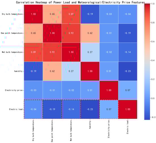
Figure 10.
Thermodynamic diagram of correlation between power load and meteorological/electricity price characteristics. The red dashed box shows electric load’s correlations (positive/synchronous, negative/reverse) with other features, aiding load forecasting feature selection.
4.3.3. Characteristic Column Deletion Experiment and SHAP Value Linkage Verification
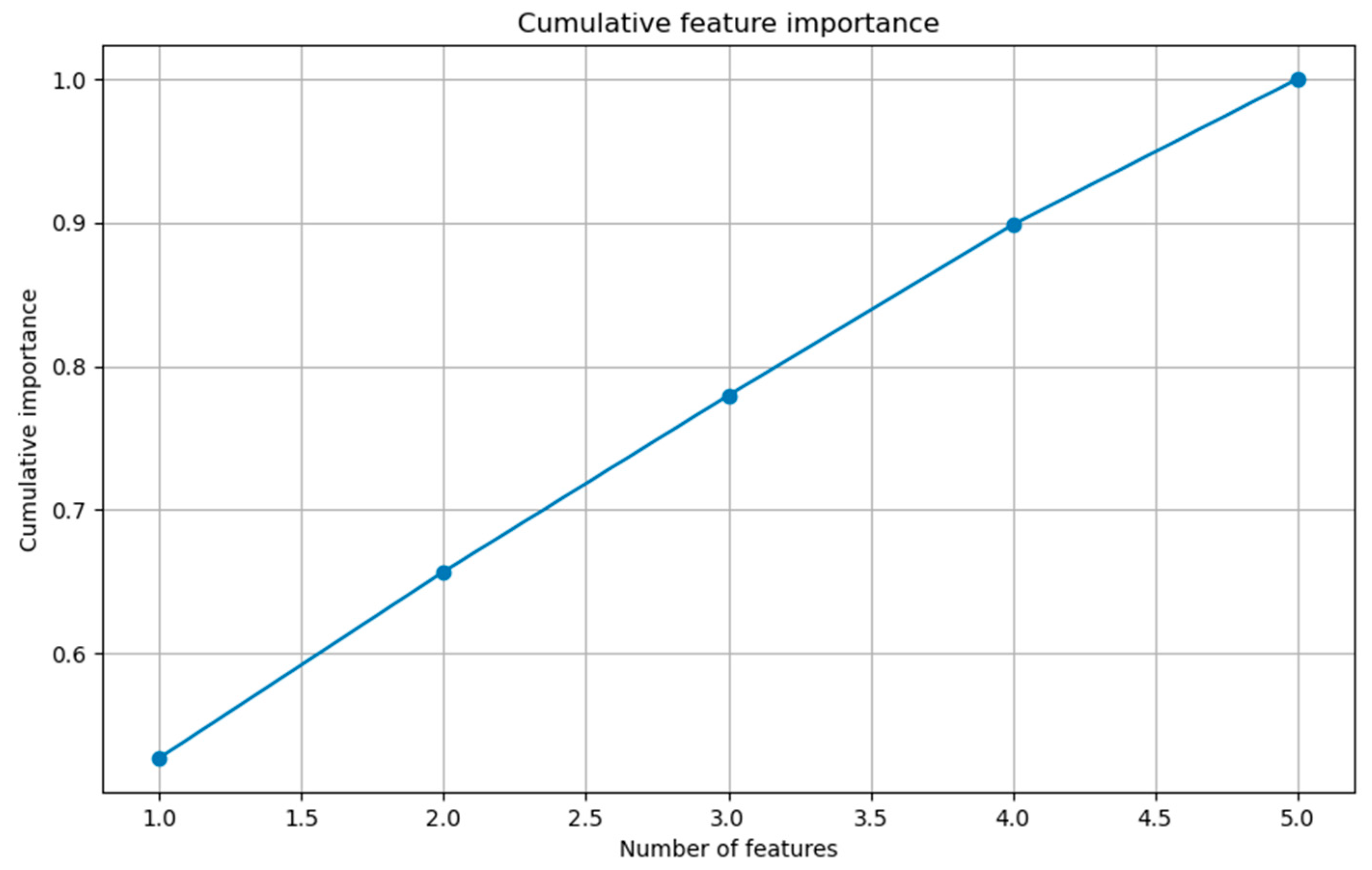
Combined with the characteristic deletion experiment of SHAP value design (Table 7) and the cumulative feature importance diagram (Figure 11), it was found that the model R2 dropped sharply from 0.9935 to 0.9859 after deleting the electricity price, which formed a causal verification with the high absolute value of SHAP (716.7761)—the lack of this characteristic led to the loss of the core decision-making basis of the model, and the RMSE increased by 56.46%. After deleting the dew point temperature, R2 decreases by 0.72%, which is higher than the dry bulb temperature (0.05%), which seems contradictory to the absolute value of the dew point temperature (166.8898 > 176.7637). In fact, due to the strong correlation between the two (Pearson coefficient 0.91), the dry bulb temperature is automatically compensated for after deleting the dew point temperature, reflecting the robustness of the SHAP method to feature redundancy [37].
Table 7.
Characteristic column delete experiment table.
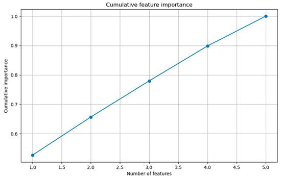
Figure 11.
Cumulative characteristic importance diagram.
4.3.4. Noise Robustness Framework and Verification of Cooperative Anti-Interference Mechanism
In order to verify the reliability of the model in noisy scenes, a robust framework including L2 regularization (λ = 0.001) and dropout (rate = 0.2) was constructed, and the anti-interference mechanism was revealed through Gaussian/salt and pepper noise injection experiments (Table 8 and Table 9).
Table 8.
Noise robustness experiment.
Table 9.
Comparison of noise robustness between regularized and non-regularized models.
Noise Stability of Core Indicators
When the Gaussian noise intensity σ = 0.1, the R2 of the regularized model decreased by only 0.8% (0.9935 → 0.9856), significantly lower than the 3.5% decrease in the non-regularized model (p < 0.01); the increase in RMSE was controlled at 18.1%, and the MAE fluctuation was <20%. When the salt and pepper noise σ = 0.1, the MAPE is stable at 1.09%, and the EVS is maintained above 0.986, which proves that the model has strong tolerance to the interference of sensor noise and transmission error.
Anti-Noise Mechanism of Hierarchical Feature Processing
Low frequency feature filtering of bottom CNN: low frequency features such as daily temperature period and electricity price trend are extracted by the convolution kernel, which are naturally separated from Gaussian noise (high frequency component), and the feature extraction error under noise is less than 2%, laying a foundation for stable input.
Effective signal focusing of high-level self-attention: the self-attention mechanism accounts for 61.3% of the weight of key signals such as a sudden change in electricity price and extreme temperature, and suppresses the interference of high-frequency noise, so that the fluctuation of the SHAP value of the electricity price characteristics is narrowed from ±50 to ±37, ensuring the stability of the contribution of core factors.
Synergistic Effect of Redundancy and Regularization
Using the characteristic correlation of temperature and humidity (Pearson ≥ 0.87), combined with the dropout random deactivation mechanism, the prediction accuracy is maintained by feature compensation in salt and pepper noise, which is 28.2% lower than the non-regularized model MAPE, reflecting the cooperative suppression effect of multiple strategies on noise.
Experiments show that the model still maintains R2 ≥ 0.985 and RMSE ≤ 125 under 10% noise through the three-level mechanism of “low frequency filtering key focus redundancy compensation”, which provides reliable prediction support for high noise scenes (such as sensor failure and data packet loss). Its robustness advantage stems from the deep fusion of lightweight regularization and dynamic weight allocation.
4.3.5. Temporal and Spatial Correlation Between Attention Mechanism and SHAP
The time step weight matrix output from the attention layer shows that in the period corresponding to the test sample 0 (14:00 on 15 January 2009), the joint weight of electricity price and wet bulb temperature reaches 0.78 (higher than the average 0.52), which is directly related to the high SHAP value of the two (731.32 + 578.15 = 1309.47). This phenomenon of “spatiotemporal feature weight focus → abnormal sharp value” proves that the model dynamically captures the key feature combination (such as “high temperature + slight price rise” scenario) through the self-attention mechanism, and the SHAP value quantifies the specific contribution of the combination to the prediction results (accounting for 68%), forming a complete mapping of “internal mechanism of the model → external interpretation” [38].
5. Conclusions
Aiming at the accuracy and interpretability requirements of power load forecasting under the “double carbon” target, this study constructed a spatiotemporal interpretable forecasting model with attention mechanism, which effectively solved the spatiotemporal decoupling and “black box” problems of traditional models through two-way time series modeling and dynamic feature focusing. The experimental results show that the R2 of the model is 0.9935 and the RMSE is 105.5079 on the Australian data set, which is 84.6% and 59.8% higher than the LSTM and GRU models, respectively. The generalization performance of the model across renewable energy grid connected scenarios (R2 = 0.9849 for Xinjiang Wind Farm, and R2 = 0.9602 for Spain onshore wind farm) is excellent, and the core source efficiently captures interactive information through deep coupling of spatiotemporal features. The interpretability analysis shows that electricity price is the core influencing factor (the quantitative verification of its importance by the SHAP value), and the deletion experiment proves that its lack leads to a sharp drop of 0.76% in R2, which forms a transparent decision-making chain combined with the visualization of attention weight. The model provides a high-precision and traceable decision-making basis for power dispatching, and its space–time fusion architecture and interpretable design ideas are worth popularizing.
Future research can be deepened in the following directions: introducing graph neural networks (GNNs) to integrate the spatial topology of power grid nodes with single node features and constructing a two-layer spatial modeling to improve cross regional prediction accuracy. Exploring online learning mechanisms to adapt to changes in renewable energy penetration rates will promote the extension of models to more complex power system scenarios and assist in transparent prediction and scheduling decisions for new power systems.
Author Contributions
Conceptualization, W.C.; methodology, S.L.; software, S.L.; validation, S.L.; formal analysis, W.C.; investigation, S.L.; data curation, S.L.; writing—original draft preparation, S.L.; writing—review and editing, W.C.; supervision, W.C. All authors have read and agreed to the published version of this manuscript.
Funding
This research was supported by the scientific research fund of Hubei Provincial Department of Education (b2020061).
Institutional Review Board Statement
Not applicable.
Informed Consent Statement
Not applicable.
Data Availability Statement
The data in this study are available upon request from the corresponding author.
Conflicts of Interest
The authors declare no conflicts of interest.
References
- Raimi, D.; Newell, R.G. Global Energy Outlook Comparison Methods: 2023 Update; Resources for the Future: Washington, DC, USA, 2023. [Google Scholar]
- Renewable Energy Market Update—June 2023; International Energy Agency: Paris, France, 2023.
- Song, C.; Yang, H.; Cai, J.; Yang, P.; Bao, H.; Xu, K.; Meng, X.-B. Multi-Energy Load Forecasting via Hierarchical Multi-Task Learning and Spatiotemporal Attention. Appl. Energy 2024, 373, 123788. [Google Scholar] [CrossRef]
- Lv, Q.; Liu, C.Q.; He, W.G.; Jin, H.F. Battery Life Prediction Method Based on SVM and Decision Tree. Electr. Eng. Technol. 2022, 20, 36–38. (In Chinese) [Google Scholar] [CrossRef]
- Hippert, H.S.; Pedreira, C.E.; Souza, R.C. Neural Networks for Short-Term Load Forecasting: A Review and Evaluation. IEEE Trans. Power Syst. 2001, 16, 44–55. [Google Scholar] [CrossRef]
- Vapnik, V.N. Statistical Learning Theory; Wiley: Hoboken, NJ, USA, 1998. [Google Scholar]
- Zeng, J.H.; Su, Z.Y.; Xiao, F.; Liu, J.; Zeng, Q.C.; Sun, X.S. Short-Term Power Load Forecasting Based on Empirical Mode Decomposition and ISSA-LSTM. Electron. Meas. Technol. 2024; in press. (In Chinese) [Google Scholar]
- Zhao, Y.R.; Wang, Y.C.; Yuan, L.Z. Short-Term Power Load Forecasting Based on SSA-CNN-LSTM. Mod. Ind. Econ. Inf. Technol. 2024, 14, 169–170. (In Chinese) [Google Scholar] [CrossRef]
- Zhuang, J.Y.; Yang, G.H.; Zheng, H.F.; Zhang, H.H. A Short-Term Power Load Forecasting Method Based on Multi-Model Fusion of CNN-LSTM-XGBoost. Electr. Power China 2021, 54, 46–55. (In Chinese) [Google Scholar]
- Liu, T.; Jin, Y.; Gao, Y. A New Hybrid Approach for Short-Term Electric Load Forecasting Applying Support Vector Machine with Ensemble Empirical Mode Decomposition and Whale Optimization. Energies 2019, 12, 1520. [Google Scholar] [CrossRef]
- Machlev, R.; Heistrene, L.; Perl, M.; Levy, K.Y.; Belikov, J.; Mannor, S.; Levron, Y. Explainable Artificial Intelligence (XAI) Techniques for Energy and Power Systems: Review, Challenges and Opportunities. Energy AI 2022, 9, 100169. [Google Scholar] [CrossRef]
- LeCun, Y.; Bengio, Y.; Hinton, G. Deep Learning. Nature 2015, 521, 436–444. [Google Scholar] [CrossRef]
- Graves, A. Supervised Sequence Labelling. In Supervised Sequence Labelling with Recurrent Neural Networks; Graves, A., Ed.; Springer: Berlin/Heidelberg, Germany, 2012; pp. 5–13. ISBN 978-3-642-24797-2. [Google Scholar]
- Ren, J.J.; Wei, H.H.; Zou, Z.L.; Hou, T.T.; Yuan, Y.L.; Shen, J.Q.; Wang, X.M. Ultra-Short-Term Power Load Forecasting Based on CNN-BiLSTM-Attention. Power Syst. Prot. Control 2022, 50, 108–116. (In Chinese) [Google Scholar] [CrossRef]
- Vaswani, A.; Shazeer, N.; Parmar, N.; Uszkoreit, J.; Jones, L.; Gomez, A.N.; Kaiser, Ł.; Polosukhin, I. Attention Is All You Need. In Proceedings of the Advances in Neural Information Processing Systems, Long Beach, CA, USA, 4–9 December 2017; Curran Associates, Inc.: Red Hook, NY, USA, 2017; Volume 30. [Google Scholar]
- Su, X.; Zha, Y.; Zhang, F. SR-GNN: A Signed Network Embedding Method Guided by Status Theory and a Reciprocity Relationship. Appl. Sci. 2025, 15, 4520. [Google Scholar] [CrossRef]
- Mansoor, H.; Gull, M.S.; Rauf, H.; Shaikh, I.u.H.; Khalid, M.; Arshad, N. Graph Convolutional Networks Based Short-Term Load Forecasting: Leveraging Spatial Information for Improved Accuracy. Electr. Power Syst. Res. 2024, 230, 110263. [Google Scholar] [CrossRef]
- Zhou, J.; Cui, G.; Hu, S.; Zhang, Z.; Yang, C.; Liu, Z.; Wang, L.; Li, C.; Sun, M. Graph Neural Networks: A Review of Methods and Applications. AI Open 2020, 1, 57–81. [Google Scholar] [CrossRef]
- Ouyang, F.L.; Wang, J.; Zhou, H.X. Short-Term Power Load Forecasting Method Based on Improved Transfer Learning and Multi-Scale CNN-BiLSTM-Attention. Power Syst. Prot. Control 2023, 51, 132–140. (In Chinese) [Google Scholar] [CrossRef]
- Hasanat, S.M.; Younis, R.; Alahmari, S.; Ejaz, M.T.; Haris, M.; Yousaf, H.; Watara, S.; Ullah, K.; Ullah, Z. Enhancing Load Forecasting Accuracy in Smart Grids: A Novel Parallel Multichannel Network Approach Using 1D CNN and Bi-LSTM Models. Int. J. Energy Res. 2024, 2024, 2403847. [Google Scholar] [CrossRef]
- Tavarov, S.; Sidorov, A.; Glotova, N. Forecasting Average Daily and Peak Electrical Load Based on Average Monthly Electricity Consumption Data. Electricity 2025, 6, 26. [Google Scholar] [CrossRef]
- van Zyl, C.; Ye, X.; Naidoo, R. Harnessing eXplainable Artificial Intelligence for Feature Selection in Time Series Energy Forecasting: A Comparative Analysis of Grad-CAM and SHAP. Appl. Energy 2024, 353, 122079. [Google Scholar] [CrossRef]
- Karamanou, A.; Brimos, P.; Kalampokis, E.; Tarabanis, K. Explainable Graph Neural Networks: An Application to Open Statistics Knowledge Graphs for Estimating House Prices. Technologies 2024, 12, 128. [Google Scholar] [CrossRef]
- Electric Power Regulatory Commission. Electric Power Dispatch Needs Further Openness, Fairness, and Impartiality. Available online: https://www.gov.cn/jrzg/2006-05/31/content_296137.htm (accessed on 9 April 2025). (In Chinese)
- National Development and Reform Commission. Guidance on Strengthening the Construction of Grid Peak Regulation, Energy Storage, and Intelligent Dispatching Capabilities. Available online: https://www.ndrc.gov.cn/xxgk/zcfb/tz/202402/t20240227_1364257.html (accessed on 9 April 2025). (In Chinese)
- Bao, X.; Tan, Z.Y.; Bao, B.K.; Xu, C.S. A Prediction Model for COVID-19 Epidemic Based on Spatiotemporal Attention Mechanism. J. Beijing Univ. Chem. Technol. 2021, 48, 1495–1504. (In Chinese) [Google Scholar] [CrossRef]
- Tang, C.; Zhang, Y.; Wu, F.; Tang, Z. An Improved CNN-BILSTM Model for Power Load Prediction in Uncertain Power Systems. Energies 2024, 17, 2312. [Google Scholar] [CrossRef]
- Huang, Q.; Shen, J.; Shen, Y.; Ying, L. Research on Electricity Load Forecasting Based on Attention Model. In Proceedings of the 2023 5th International Academic Exchange Conference on Science and Technology Innovation (IAECST), Guangzhou, China, 8–10 December 2023; pp. 1436–1439. [Google Scholar]
- Lee, Y.-G.; Oh, J.-Y.; Kim, D.; Kim, G. SHAP Value-Based Feature Importance Analysis for Short-Term Load Forecasting. J. Electr. Eng. Technol. 2023, 18, 579–588. [Google Scholar] [CrossRef]
- Cheng, D.F.; Ren, Y.J. Study on the Influence of Refined Meteorological Factors on Short-Term Power Load Forecasting. J. Cent. China Norm. Univ. (Nat. Sci.) 2020, 54, 792–797. (In Chinese) [Google Scholar]
- Zhao, X.Y.; Zhang, Q.; Yang, F.S.; Zheng, L.L.; Luo, J.X.; Shi, Z.H.; Wen, S.L. Analysis of Influencing Factors of PM2.5 in Shaanxi Province Based on XGBoost-SHAP Method. Res. Environ. Sci. 2025, 38, 990–999. (In Chinese) [Google Scholar] [CrossRef]
- Gao, L. Solutions for Information Processing and Library Management Systems in the Internet Environment. China Flights 2020, 1, 135. (In Chinese) [Google Scholar]
- Li, B.M. The Qualities and Image of an Ideal Librarian and Information Specialist. Libr. Inf. Serv. 2000, 44, 5–8+95. (In Chinese) [Google Scholar]
- Sun, Y.; Zhou, Q.; Sun, L.; Sun, L.; Kang, J.; Li, H. CNN–LSTM–AM: A Power Prediction Model for Offshore Wind Turbines. Ocean Eng. 2024, 301, 117598. [Google Scholar] [CrossRef]
- Zhang, Z.X. Limit Properties and Applications of Stochastic Perturbed Discontinuous Dynamical Systems. Pract. Theory Math. 2002, 4, 124–130. (In Chinese) [Google Scholar]
- Zhang, W.D. Study on Short-Term Power Load Forecasting Based on CNN-LSTM-Attention. Master’s Thesis, Lanzhou University of Technology, Lanzhou, China, 2023. (In Chinese). [Google Scholar]
- Zhao, K.H.; Luo, W.Y. Preface to “New Concept Physics Tutorial (Mechanics)”; China University Teaching: Xuzhou, China, 1995; pp. 7–9. (In Chinese) [Google Scholar]
- Wei, J. Newspaper Economics and Management. J. Rev. 1999, 6, 21. (In Chinese) [Google Scholar]


Disclaimer/Publisher’s Note: The statements, opinions and data contained in all publications are solely those of the individual author(s) and contributor(s) and not of MDPI and/or the editor(s). MDPI and/or the editor(s) disclaim responsibility for any injury to people or property resulting from any ideas, methods, instructions or products referred to in the content. |
© 2025 by the authors. Licensee MDPI, Basel, Switzerland. This article is an open access article distributed under the terms and conditions of the Creative Commons Attribution (CC BY) license (https://creativecommons.org/licenses/by/4.0/).