Article

NCC—An Efficient Deep Learning Architecture for Non-Coding RNA Classification

by
Konstantinos Vasilas
1,
Evangelos Makris
2,*,
Christos Pavlatos
3 and
Ilias Maglogiannis
1
1
Department of Digital Systems, University of Piraeus, 18534 Piraeus, Greece
2
School of Electrical and Computer Engineering, National Technical University of Athens, 9 Iroon Polytechniou St, 15780 Athens, Greece
3
Department of Informatics and Computers, Hellenic Air Force Academy, Dekelia Air Base, Acharnes, 13671 Athens, Greece
*
Author to whom correspondence should be addressed.
Technologies 2025, 13(5), 196; https://doi.org/10.3390/technologies13050196
Submission received: 26 March 2025 / Revised: 26 April 2025 / Accepted: 5 May 2025 / Published: 12 May 2025
(This article belongs to the Special Issue Breakthroughs in Bioinformatics and Biomedical Engineering)

Abstract

:
In this paper, an efficient deep-learning architecture is proposed, aiming to classify a significant category of RNA, the non-coding RNAs (ncRNAs). These RNAs participate in various biological processes and play an important role in gene regulation as well. Because of their diverse nature, the task of classifying them is a hard one in the bioinformatics domain. Existing classification methods often rely on secondary or tertiary RNA structures, which are computationally expensive to predict and prone to errors, especially for complex or novel ncRNA sequences. To address these limitations, a deep neural network classifier called NCC is proposed, which focuses solely on primary RNA sequence information. This deep neural network is appropriately trained to identify patterns in ncRNAs, leveraging well-known datasets, which are publicly available. Additionally, a ten times larger dataset than the available ones is created for better training and testing. In terms of performance, the suggested model showcases a 6% enhancement in precision compared to prior state-of-the-art systems, with an accuracy level of 92.69%, in the existing dataset. In the larger one, its accuracy rate exceeded 98%, outperforming all related tools, pointing to high prediction capability, which can act as a base for further findings in ncRNA analysis and the genomics field in general.

1. Introduction

Non-coding RNAs (ncRNAs) are a type of RNA that contributes to various essential molecular procedures. When these aspects arose, many researchers identified many potential challenges, and their identification has become of main interest in the field of biology and bioinformatics. Due to these significant functions, the accurate prediction of the families associated with different ncRNAs was published in the literature using experimental and computational methods. Conventional experimental methods such as in [1] were proposed, but the fact that they are time-consuming, labor-intensive, and expensive led the research to computational ones. The two main categories are the Sequence or Secondary Structure-based Methods and the Homologous Sequence Alignment Methods. The first methods analyze the 1D or 2D structure of ncRNAs to classify them accordingly. The main disadvantage of these methods is that their accuracy is bound by the predicted secondary structures, which is a standalone, hard task to accomplish. The second approach, as presented in [2], aligns ncRNAs with their homologues to identify common characteristics and, according to those, predict their families. This method performs very well in many cases, but is bound by an accurate secondary structure annotation for the sequences and is not capable of handling pseudoknotted structures. NCC architecture is directed toward the classification of ncRNA sequences by means of deep learning. RNA sequences can be submitted to the model and no further information is required. The architecture consists of a convolution layer with a pooling layer to downsize the data. Next, a bidirectional RNN layer is used to analyze possible patterns forward and backward. Finally, a fully connected layer integrates all elements produced and generates the final prediction. The primary aim of NCC is to establish a deep learning-based architecture where high accuracy and faster training results can be achieved. The NCC model suggested herein operates exclusively on primary sequence data and uses a sparse deep learning architecture. Through the absence of structural inputs, NCC avoids preprocessing overheads and promotes generalization without compromising on superior classification performance. Such simplicity, efficiency, and accuracy-focused methodology is the central contribution of this research. Considering the state-of-the-art approaches adopted in the domain, problems to be solved, and the steps already accomplished, this work intends to provide biologists and bioinformaticians with the most needed information and skills to create more intelligent, more precise, and faster functioning ncRNA classifiers. The proposed method and the constructed dataset are publicly available under the NCC GitHub repo [3].

1.1. RNA

Ribonucleic acid, or RNA for short, is a molecule involved in biological activities. It is involved in the control of information, gene expression, and protein synthesis. RNA is a single-stranded molecule made of nucleotides. A base (adenine, cytosine, guanine, or uracil), a sugar known as ribose, and a phosphate group make up each nucleotide. In short, transcription is the process by which DNA is converted into RNA, which assists in converting the code into proteins. The cell’s ability to perform essential duties for the organism’s general health and optimal operation depends on many forms of RNA, including messenger RNA (mRNA), transfer RNA (tRNA), ribosomal RNA (rRNA), and small nuclear RNA (snRNA):
  • From DNA, messenger RNA (mRNA) is created. It transfers information to the ribosomes found in the cytoplasm from the nucleus. It is translated at the ribosomes, where protein synthesis occurs.
  • Transfer RNA (tRNA) is a molecule that carries amino acids to the ribosomes during protein synthesis. Using mRNA codons, which are three nucleotide sequences that encode different amino acids, to match acids, this operation is accomplished. Then, these acids are incorporated into the expanding chain.
  • A component of ribosomes, which are cellular structures in charge of protein synthesis, is ribosomal RNA (rRNA). In addition to supporting ribosomes, rRNA aids in accelerating chemical events that result in the synthesis of proteins.
  • A class of RNA molecules that support cellular functions includes small nuclear RNA (snRNA). Participating in RNA splicing, which entails cutting out coding sections from mRNA called introns and putting together coding sequences called exons, is one of its roles.

1.2. Non-Coding RNA

An important type of RNA that has been identified is ncRNA [4], which plays a key role and should not be overlooked whenever cellular mechanisms are discussed. Even though the original idea surrounding RNA revolved around the transfer of information for the creation of proteins, the reality of ncRNAs came to be that they were non-protein coding themselves, yet impacted protein activities along with gene regulation, and were involved in other biological functions too. ncRNAs are categorized in regard to their size and function. MicroRNAs (miRNAs) and small interfering RNAs (siRNAs) are examples of small non-coding RNAs (ncRNAs), which are typically shorter than 200 nucleotides. Both of these RNAs are essential for RNA interference, which is a vital step in the silencing of genes following transcription. Long non-coding RNAs (lncRNAs) are a different subgroup that is longer than 200 nucleotides and has a variety of regulatory roles, including altering the structure of chromatin and regulating transcriptional activity. Moreover, transfer RNAs (tRNAs) and ribosomal RNAs (rRNAs), which are widely recognized for their roles in protein synthesis, are also categorized as non-coding RNAs. This demonstrates that the genome contains coding sequences. Thirteen classes of ncRNA families are registered in Rfam [5], which have been employed in this work as well as numerous other studies. A total of 10% of RNAcentral [6] sequences, as reported in [7], do not belong to any known Rfam family and may be members of new families. Specific examples of the classes of ncRNAs that make up this number are the piRNAs and siRNAs, which, with one minor exception, comprise 5% of this total. In summary, neither of these classes is structurally relevant for inclusion in Rfam for effective structure modeling. To understand the function of an RNA molecule and design RNA molecules with specific functions, it is essential to predict their secondary structure. Numerous computational tools, including Knotify [8] and its variations [9,10,11], Knotty [12], IPknot [13], Hotknots [14], and Probknot [15] are capable of predicting the secondary structure of RNAs. These tools use a variety of techniques to tackle this task with respect to the sequence of interest. The three-dimensional structure of an RNA molecule is crucial for its function. The tertiary structure of RNA is made up of more complex folding, in which different parts fold in complex ways, as opposed to the basic structure of nucleotides or the secondary structure of simple loops and helices. Interactions between the RNA molecule’s component parts, such as base pairs, which are widely spaced in the molecule, have an impact on this folding process. The form that this folding yields determines the function of the RNA, which includes its participation in the control of gene expression, protein synthesis, and other cellular processes. All these different structures of RNA are usually used to train the models for the classification of the non-coding RNAs, which is the task that this study is focused on. In the literature, which is analyzed in the following section, many systems utilize the primary, secondary, or tertiary structure of the molecule, or a combination of them, to enhance their performance.

2. Related Work

An important issue in genomics is the classification of ncRNAs because of their contribution to a variety of biological processes. A number of computational techniques have been developed recently to enhance the precision of this task. Some of these technologies stand out because of their distinct advantages and are presented in this section. RNAcon [16] is a tool that leverages structure and sequence alignment data to classify non-coding RNAs. Because of its dual methodology, RNAcon is capable of classifying and identifying several kinds of non-coding RNAs with remarkable accuracy, especially when it comes to secondary structures and conserved RNA motifs. Graph-based deep learning approaches have also been employed in the last few years for ncRNA classification, as seen in [17,18]. The models typically map RNA sequences onto graphs, with nucleotides as vertices and their interactions as edges, representing both sequential and structural information. While such approaches have demonstrated promising performance through the employment of complex topological properties, they often require secondary structure information or advanced preprocessing steps to construct the graphs. Another graph-based depiction of RNA sequences is presented by GraPPLE (Graph-based Prediction of ncRNA using Pairwise Labeled Edges) [19], in which nucleotides are described as nodes and their interactions as edges. GraPPLE effectively captures complex structural links seen in RNA sequences, achieving high classification accuracy, particularly for newly discovered or poorly defined ncRNA families. NCodR [20] is a multi-class support vector machine classifier for identifying non-coding RNAs in plants, using distinct regions in the distribution of AU and minimum folding energy as additional attributes. Another classifier has been proposed, called MncR [21]. This approach evaluates different approaches by utilizing primary sequences and secondary structures, using different neural network architectures. The ncRFP system [22], or non-coding RNA Feature Predictor, extracts and chooses pertinent characteristics for ncRNA classification. Large-scale genomic research frequently deals with high-dimensional data, which ncRFP excels at managing through the use of a random forest classifier. The tool’s excellent prediction accuracy is a result of its capacity to include various sequence-based and structural characteristics. Deep learning methods are also used to tackle this task. Convolutional neural networks (CNNs) are adept at capturing local motifs and patterns in sequences but are incapable of modeling long-range dependencies. Recurrent neural networks (RNNs), and, in particular, Long Short-Term Memory (LSTM) and Gated Recurrent Unit (GRU) variants, are well suited to model sequential dependencies, with particular suitability for biological time-series or sequence data [23]. However, they can suffer from vanishing gradients and slow training times. Architectures based on Transformers [24,25] have gained a lot of attention recently due to their parallelism and ability to model global dependencies via self-attention mechanisms. They often require lots of data and a lot of computational resources, which, in biological terms, are not always available. Next, some of the most well-known works related to ncRNA classification are presented. nRC (non-coding RNA classifier) [26], for example, is able to discriminate between coding and non-coding RNAs. High sensitivity and specificity are demonstrated by this method. It integrates sequence-based characteristics with deep neural networks, especially in the differentiation of closely related RNA families. In another work, Residual networks, or ResNets, are used by ncDLRES (non-coding RNA Deep Learning Residual Network) [27] to classify ncRNAs. By addressing the degradation, this deep learning strategy improves the classification level. ncDLRES is well suited for genome-wide classification tasks because of its exceptional efficacy in handling sizable and intricate datasets. Similarly, ncDENSE (non-coding RNA Dense Network) [28] identifies complex patterns in RNA sequences using dense neural networks. The model can identify novel ncRNAs, even in cases where the available data for training are deficient. ncDENSE can reliably classify data under a range of circumstances with high accuracy. Finally, incorporating a variety of deep learning models, including recurrent neural networks (RNNs) and convolutional neural networks (CNNs), BioDeepfuse [29] is a state-of-the-art framework for classifying non-coding RNAs. BioDeepfuse captures long-range relationships and local sequence patterns within RNA sequences by merging these models. A review of the other similar systems, which leverage machine learning techniques for this task, is also shown in [30].

3. Implementing the Prediction Mechanism

The paper’s implementation of the ncRNA classification model is the main topic of this part. This section, which is broken down into multiple parts, describes the procedures used to prepare the data, create the model architecture, train the model, and assess it. This paper aims to create a ncRNA classifier that uses the primary structure as its input. The errors of secondary structure prediction methods (graph characteristics) are not included in the classification flow, since the focus is solely on the primary structure of the RNA. Thus, the core contribution of this paper is focused on the development of an ncRNA classifier with the following elements:
1.
The model’s input is the primary structure of RNA.
2.
The proposed model should be simple, like ncRFP [22], for short training periods.
3.
High level of accuracy for all prediction-related metrics.

3.1. Data Preparation

The preparation of the data was conducted in two stages. The first stage was dedicated to padding and cutting the sequences when necessary, to homogenize the input data. The second one applied to all RNAs the one-hot encoding to prepare a format easy to interpret by the neural network.

3.1.1. Data Preprocessing

Padding and cutting are common methods for the preparation of sequences ready for use in deep learning models. This is quite common in problems including sequential data tasks like speech recognition and natural language processing (NLP). By verifing a consistent length for each sequence, the model’s validity and efficiency is ensured in terms of the computational aspect and homogeneity. To create a dataset with sequences of equal length, additional components can be used. Usually, zero padding or filler values are used for this task. The model is designed in such a way that features are learned from sequences of all lengths, which helps reduce overfitting risk. In this case, cutting was applied for the longest sequences, and specifically, the final parts in the sequence were eliminated. In that way, better memory usage was achieved, while, at the same time, the model was not too complex and difficult to train.
By inspecting Figure 1, it is apparent that the majority of the sequence has less than 500 nucleotides. So, it was decided that the input sequence for NCC would be 500 lengths. This means that sequences made up of fewer than 500 nucleotides would be artificially padded with 0 s, while sequences with more than 500 would be truncated, running the risk of ignoring some important sequence features. It is acknowledged that padding and truncation processes can introduce redundancy or cause partial loss of sequence information. However, the high classification accuracy across all classes suggests that whatever loss of information occurred in padding/truncation did not adversely affect the accuracy of the model.

3.1.2. One-Hot Encoding

In machine learning, categorical data need to be prepared by transforming categories into binary vectors with one-hot encoding. This avoids the suggestion of an incorrect hierarchy that would result from assigning some random numeric values (e.g., 1, 2, 3) that might be incorrectly interpreted as a significant order by certain algorithms. The main advantage is that it preserves category uniqueness without suggesting any order. However, when there are many categories, it can incredibly increase the feature space, with added computational expense and risk of overfitting. Therefore, it is usually used selectively or combined with dimensionality reduction techniques.
In this case, there were 16 possible characters to represent, as explained in Table 1, but most of them were either absent or very rare in the dataset. To this end, to encode the data, the four RNA bases were described accordingly, while additional IUPAC characters were represented by ’X’, which was also the character used for padding. Table 2 depicts the encoding of characters to four and eight digits. This approach was selected over the full IUPAC 16-character encoding because the NCC and nRC datasets include only a very limited number of the remaining characters listed in Table 1.

3.2. NCC Model Architecture

For the scope of this study, 25 unique models were evaluated in the NCC dataset. A set of experiments that involved dense networks and convolutional networks as standalone networks and in a sequential way was conducted. But, finally, it was the recurrent models that were fitted with a bidirectional neural network (BiRNN) [31] that performed the best in accuracy among all types of networks tested. Recent investigations have demonstrated that bidirectional RNN outperforms its counterparts, such as standard RNN, in learning sequential data by moving through the sequence in both directions. This is important for understanding the RNA case because, in most cases, it is determined by the neighboring nucleotides on either side of it. Nonetheless, a huge amount of context or patterns can be easily overlooked if typical RNNs are solely applied because RNNs operate in one direction. A BiRNN is a two-directional approach where the RNA sequence is estimated by looking at the nucleotides in the center and both ends. Its flexibility to be able to see the sequence dependencies in all possible places gives a better appreciation of how the RNA is structured and its functioning. The unique classification of BiRNNs gives it an upper hand over other sequence order tasks such as RNA classification. The model with the highest prediction capability and tolerable loss margins while maintaining a fairly simple architecture is presented. It comprises a one-dimensional convolutional neural network, a one-dimensional max pooling layer, a bidirectional recurrent layer, and a fully connected layer. The neural network is presented in Figure 2.
The convolutional layer scans for essential features in the input data, while the max pooling layer reduces the size of the feature map by downsampling. The bidirectional recurrent layer captures long-range dependencies within the input, and this is combined in the fully connected dense layer to output an ultimate prediction. The model reaches the highest accuracy with this neural network, while keeping an acceptable loss in the NCC dataset. Since these experiments have shown its application across a wide variety of classification of sequential data tasks in the NCC dataset. The presented structure was implemented in Keras [32], representing a neural network capable of categorizing sequence information into 13 types by identifying 13 units and a ’softmax’ activation function at its very end. The model then takes an input layer of a sequence with a dimensionality of either (500, 4) or (500, 8), with 500 being the length of the padded and truncated sequence, while 4 or 8 is the number of features, depending on the number of features used in one-hot encoding. That translates to sequences of length 500 with four or eight features each. This is followed by a one-dimensional convolutional layer, which uses 32 filters of size 9 with ReLU for the activation function to extract meaningful features from the sequence data. The max pooling layer reduces dimensionality by pooling over windows of size 4, therefore condensing the data while retaining key features and reducing computational complexity. Next, this is passed through a bidirectional GRU layer with 128 units to capture contextual dependency in both directions. Thus, it contains a dropout of 0.3 and initialization using randomized initializers for kernels and recurrent weights, but with zeros as biases. The output from the GRU layer is then flattened into a single-dimensional format through a flattening layer, thereby preparing it for the fully connected dense layers. Finally, it ends with a dense layer composed of 13 units and the ’softmax’ activation function, which gives the probability distribution across the 13 classes. Hyperparameters such as the kernel size in the convolutional layer (set to 9) and the number of units in the bidirectional GRU layer (set to 128) were selected through empirical experimentation, including variations in filter size (3, 5, 7, 9), GRU units (64, 128, 256), and layer combinations. The chosen setup provided the best trade-off between training speed, generalization ability, and classification accuracy in the validation data. This study highlights both accuracy and efficiency during training and testing. The streamlined architecture facilitates rapid processing, allowing models to be trained and tested efficiently without compromising accuracy. The balance of speed and precision is a key focus of this research.

3.3. Data Collection

The Rfam database [5] was used to compile small non-coding RNA sequences, which are stored in a plain text file in the standard FASTA format. FASTA is a widely accepted text-based format in bioinformatics for representing sequences from DNA or RNA and for representing amino acid sequences of proteins. The FASTA file consists of sequence records with sequence definition lines and sequence data. Each definition line begins with a greater-than symbol (“>”) followed by some unique identifier, often a descriptive name or code. The sequence data are single-letter codes representing individual nucleotides or amino acids. Because the focus of this chapter is classification, only class information was included in the definition line of each sequence. For better understanding, an illustrative set of examples is shown below.
>IRES
ATACCTTTCTCGGCCTTTTGGCTAAGATCAAGTGTAGTATCTGTTCTTAT…
>tRNA
GCACCACTCTGGCCTTTTGGCTTAGATCAAGTGTAGTATCTGTTCTTATT…
>tRNA
ATACCTTTCTCGGCCTTTTGGCTAAGATCAAGTGTAGTATCTGTTTTTAT…
>riboswitch
ATTACTTCTCAGCCTTTTGGCTAAGATCAAGTGTAATAAATCTCATTGTG…
>HACA-box
CCAGCTCTCTTTGCCTTTTGGCTTAGATCAAGTGTAGTATCTGTTCTTTT…
>tRNA
ACAGCTGATGCCGCAGCTACACTATGTATTAATCGGATTTTTGAACTTGG…

3.4. Final Dataset (NCC Dataset)
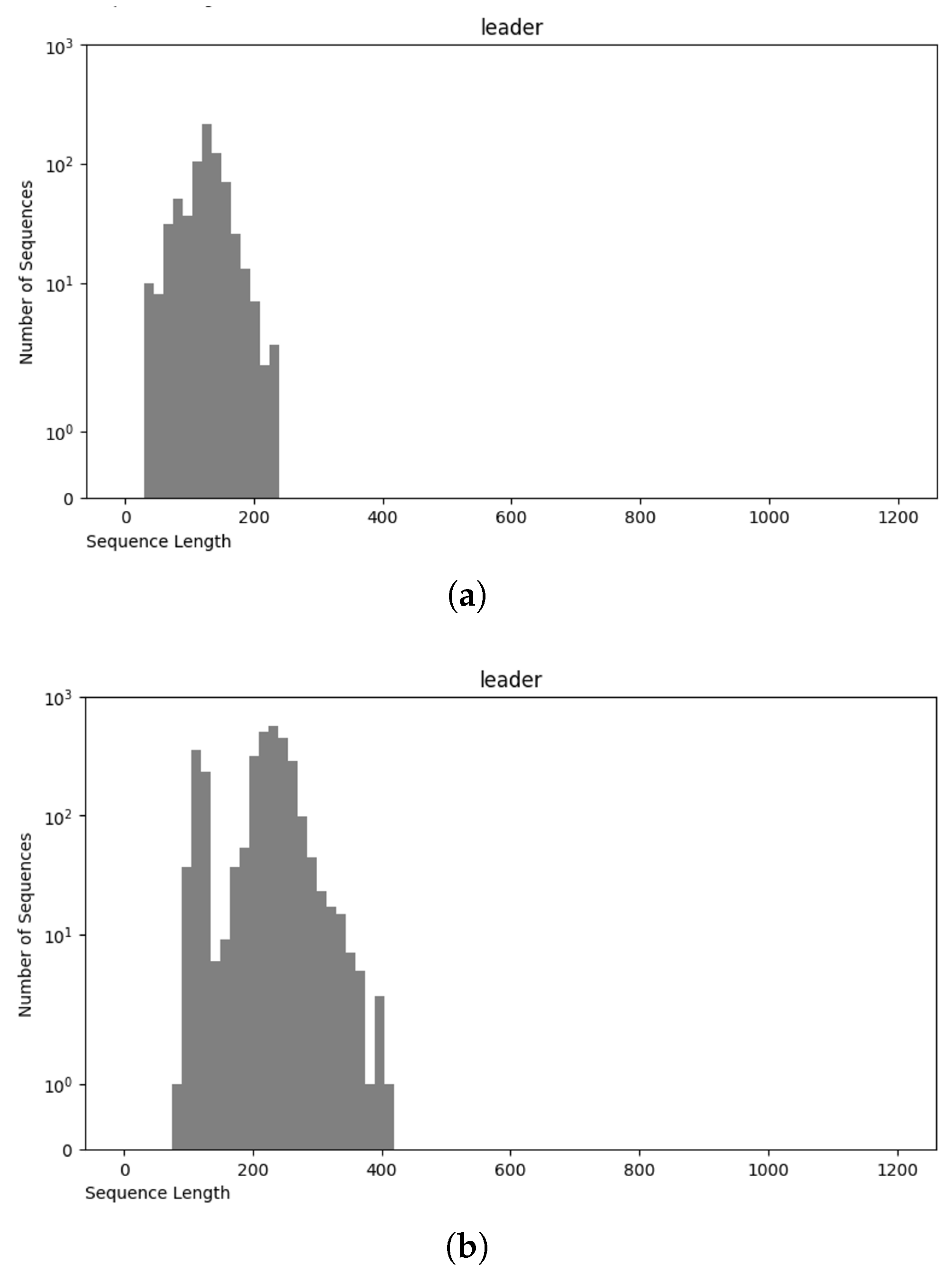
To create the final dataset, files belonging to the same family were merged to create a single .fasta file for each family. Due to the limited data regarding the IRES non-coding RNA family, a second data source was used, called IRESbase [33], which is dedicated to this family. In Table 3, the source and count of RNAs of each family are presented.
The final dataset has about 2500–5000 sequences per family. The distribution of data can be seen in Figure 3, while the number of sequences per class is presented in Table 4. To avoid introducing class imbalance and training bias, random downsampling was applied to the overrepresented RNA families, capping each class to approximately 2500–5000 sequences. This range was selected to match the lower-data families (e.g., IRES, Intron_gpI) while still retaining a sufficiently large dataset for robust training. The selection was performed using uniform random sampling without replacement, and all selected sequences met minimum quality and length requirements.
Analysis of the RNA sequence length distribution, as depicted in Figure 4, reveals a correlation between the sequence length and the class of RNA. This relationship can potentially improve the performance of the classifiers. For instance, as shown in Figure 5a, miRNA sequences are typically shorter than 200 nucleotides, whereas in Figure 5b, ribozyme RNA sequences often exceed 800 nucleotides. These values indicate that incorporating the length into classification models could be beneficial to distinguish the classes. Understanding the variation in the lengths of the RNA sequences of different classes enhances our knowledge of their structure while, at the same time, contributing to the development of more accurate and efficient RNA classifiers.

3.5. nRC Dataset

The dataset used in the nRC [26] was specifically curated for classifying non-coding RNA (ncRNA) sequences. This dataset was assembled using sequences from the Rfam database and includes 13 different ncRNA classes: miRNA, 5S rRNA, 5.8S rRNA, ribozymes, CD-box, HACA-box, scaRNA, tRNA, Intron gpI, Intron gpII, IRES, leader, and riboswitch. To ensure a balanced set of data and maintain statistical significance, a process used in previous works was applied. The CD-HIT tool [34] was utilized to select 20% non-redundant sequences, thereby avoiding redundancy that could bias the classification results. For most ncRNA classes, 500 sequences were randomly chosen, except for the IRES class, which only had 320 available sequences. This resulted in a total of 6320 ncRNA sequences in the dataset. In addition, a second dataset consisting of 2600 sequences, with 200 sequences from each class, was downloaded from Rfam to test the nRC tool. Since this dataset is normally used for benchmarking against other classification architectures, it was also adopted for training and testing the proposed model to ensure an equitable comparison, as illustrated in Figure 6.

Comparative Analysis of NCC and nRC

The NCC dataset used in this work is significantly larger, including more than an order of magnitude more sequences than the earlier dataset, nRC. Indeed, the distribution of RNA classes is rather similar between the NCC dataset and the nRC dataset, with this resemblance being very apparent for some RNA classes, such as IRES sequences, ribozymes, and Intron_gpI, which are generally longer in both datasets, though minor variations exist, as depicted in Figure 7 and Figure 8. However, a notable difference arises in the leader family, as highlighted in Figure 9, which provides a side-by-side comparison of the sequence length distribution for the leader RNA class in both sets.

3.6. Preparing and Benchmarking the Model

The Adam optimization algorithm [35] was employed with a learning rate of 0.001. Adam is a widely used method for training neural networks as it leverages the advantages of Stochastic Gradient Descent (SGD) and RMSProp, making it well-suited for handling sparse gradients in noisy environments. “Adam”, short for “Adaptive Moment Estimation”, leverages squared gradients to adapt the learning rate, similar to RMSProp, while also using the moving average of gradients, akin to SGD with momentum, rather than relying solely on the raw gradients. This synergy enables dynamic learning rate adjustment and gradient smoothing, facilitating efficient convergence toward the global minimum in the optimization process. Adam is particularly valued for its memory efficiency and computational cost-effectiveness, specifically with large datasets and many parameters. Categorical Cross-Entropy is a loss function commonly used for multi-class classification problems in machine learning. It quantifies the difference between two probability distributions, one being the actual or true distribution of the real labels, and the other being a predicted distribution generated by the model. The loss calculates the negative logarithm of the probability related to the correct class. This method is especially effective when the model’s output is a probability distribution across multiple classes, as seen in neural networks with a softmax activation function in the output layer. Categorical Cross-Entropy is essential for models requiring accurate probability distributions, particularly in multi-class classification. This loss function is calculated by the formula below:
L = i = 1 M y i log ( p i )
And, for multi-class classification,
L = i = 1 M y o , i log ( p o , i )
where the following definitions apply:
  • L is the loss.
  • M is the number of classes.
  • y i is a binary indicator (0 or 1) of whether class label i is the correct classification for the observation.
  • p i is the predicted probability of the observation belonging to class i.
  • y o , i is a binary indicator (0 or 1) of whether class i is the correct classification for observation o.
  • p o , i is the predicted probability of observation o being of class i.
To efficiently train the model, three different sets of epochs: 20, 50, and 100 were applied. Analyzing the data in Figure 10, it is obvious that, after the first 20 epochs, the model’s accuracy reaches a plateau, exhibiting minimal to no additional improvement. This pattern is also mirrored in the loss function metrics. A detailed analysis of the training process is shown in Table 5.

3.6.1. Performance Indicators

To evaluate the effectiveness of each prediction method for ncRNA classes, a set of well-established metrics is presented. Specifically, those of accuracy, sensitivity, precision, F1-score, Matthews correlation coefficient (MCC), and the confusion matrix were chosen for this task:
  • Accuracy is the percentage of correctly classified cases.
  • Sensitivity, also known as Recall, is the ratio of accurately anticipated positive cases to all actual positive cases.
  • Precision is the ratio of correctly predicted positive cases to the total predicted positive cases.
  • The F1-score is the harmonic mean of a model’s precision and recall.
  • The Matthews correlation coefficient (MCC) is an effective metric for unbalanced classes, well-known for evaluating this task.
Although the NCC dataset was constructed to include approximately 2500 to 5000 sequences per RNA family, there was minimal class imbalance. To verify whether the imbalance affected the performance of the model, classification metrics per class (i.e., precision, recall, and F1-score) were monitored. The result indicated that the model performed well across all classes without a significant decline in minority classes. As such, a class weighting or oversampling of data was not applied to the process.
In multi-class classification, accuracy is calculated as a proportion of correctly classified instances in relation to all the instances in the dataset. For other measures such as precision, recall, or F1-score, the scores for a metric are first obtained individually in each class and later averaged through macro-averaging. Macro-averaging has various benefits in multi-class classification. By calculating metrics such as precision, recall, and F1-score for each class separately and then averaging the results, macro-averaging assigns an equal weight to all classes, regardless of their frequency. This ensures that performance against minority or underrepresented classes is not dominated by majority classes, giving a balanced and unbiased assessment. Therefore, macro-averaged measures give a broad-picture view of model performance on all classes and can disclose inadequacies that average accuracy will miss. Macro-averaged metrics are also useful in model comparison because they focus on stable performance on all classes rather than weighting results towards the most common ones. Macro-averaging as a target for evaluation encourages models to perform well on the whole class range, producing more equitable and robust classification.
An example of precision computation can be seen in Formulas (3) and (4).
P r e c i s i o n C l a s s A = T P C l a s s A T P C l a s s A + F P C l a s s A
P r e c i s i o n M a c r o A v e r a g e = P r e c i s i o n C l a s s A + . . . + P r e c i s i o n C l a s s N N
In multi-class classification, the Matthews correlation coefficient (MCC) can be defined in terms of a confusion matrix C for K classes. To simplify the definition, consider the following intermediate variables:
  • t k : the number of times class k truly occurred
    t k = i K C i k
  • p k : the number of times class k was predicted
    p k = i K C k i
  • c: the total number of samples correctly predicted
    c = k K C k k
  • s: the total number of samples
    s = i K j K C i j
Then, the multi-class MCC is defined as
M C C = c × s k K p k × t k ( s 2 k K p k 2 ) × ( s 2 k K t k 2 )
It is required to remove any bias in the multi-task classification process, so each measure is computed for every class label independently. For a class C k , any instance belonging to that class is marked as positive, while any instance belonging to any other class is marked as negative.

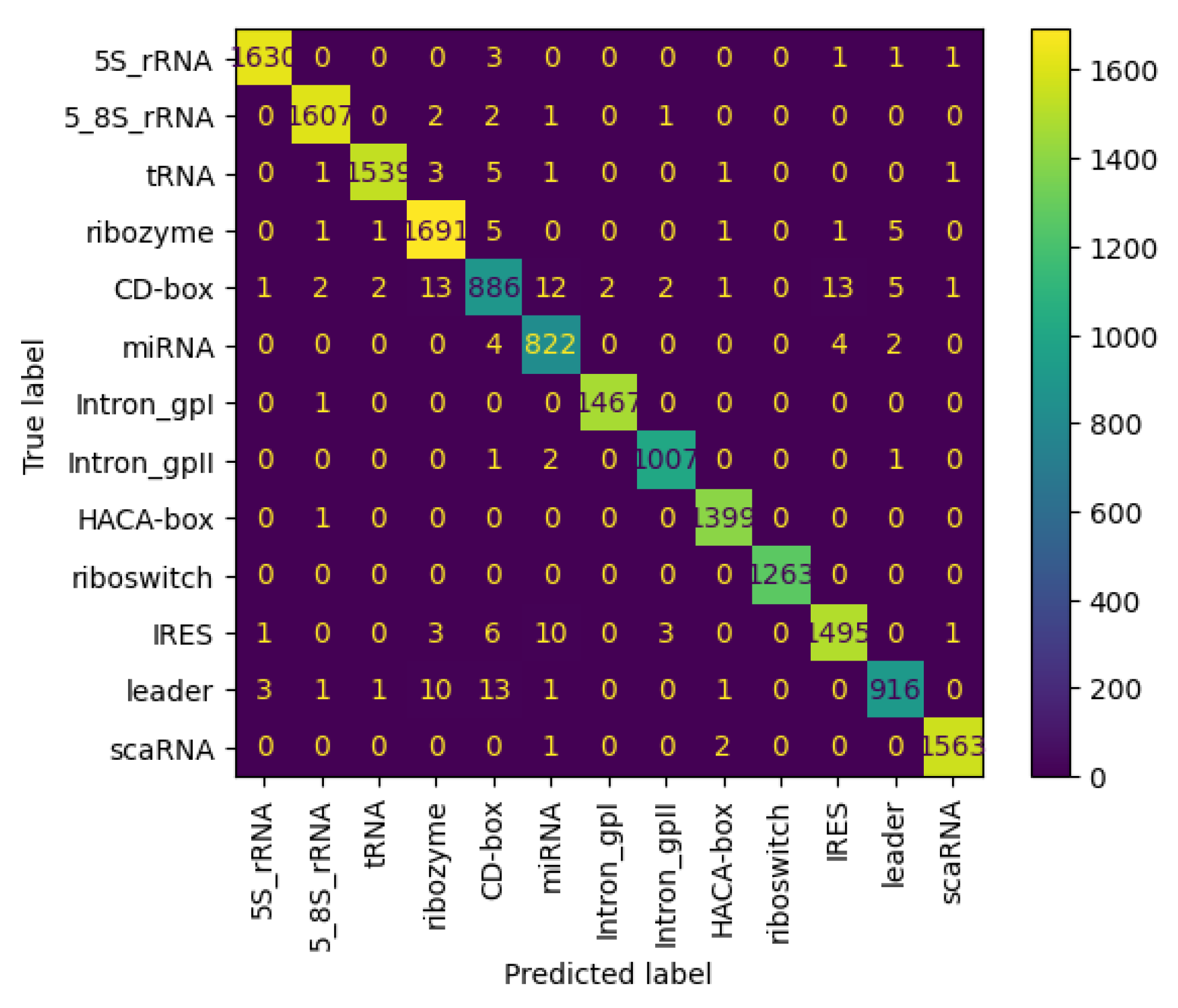
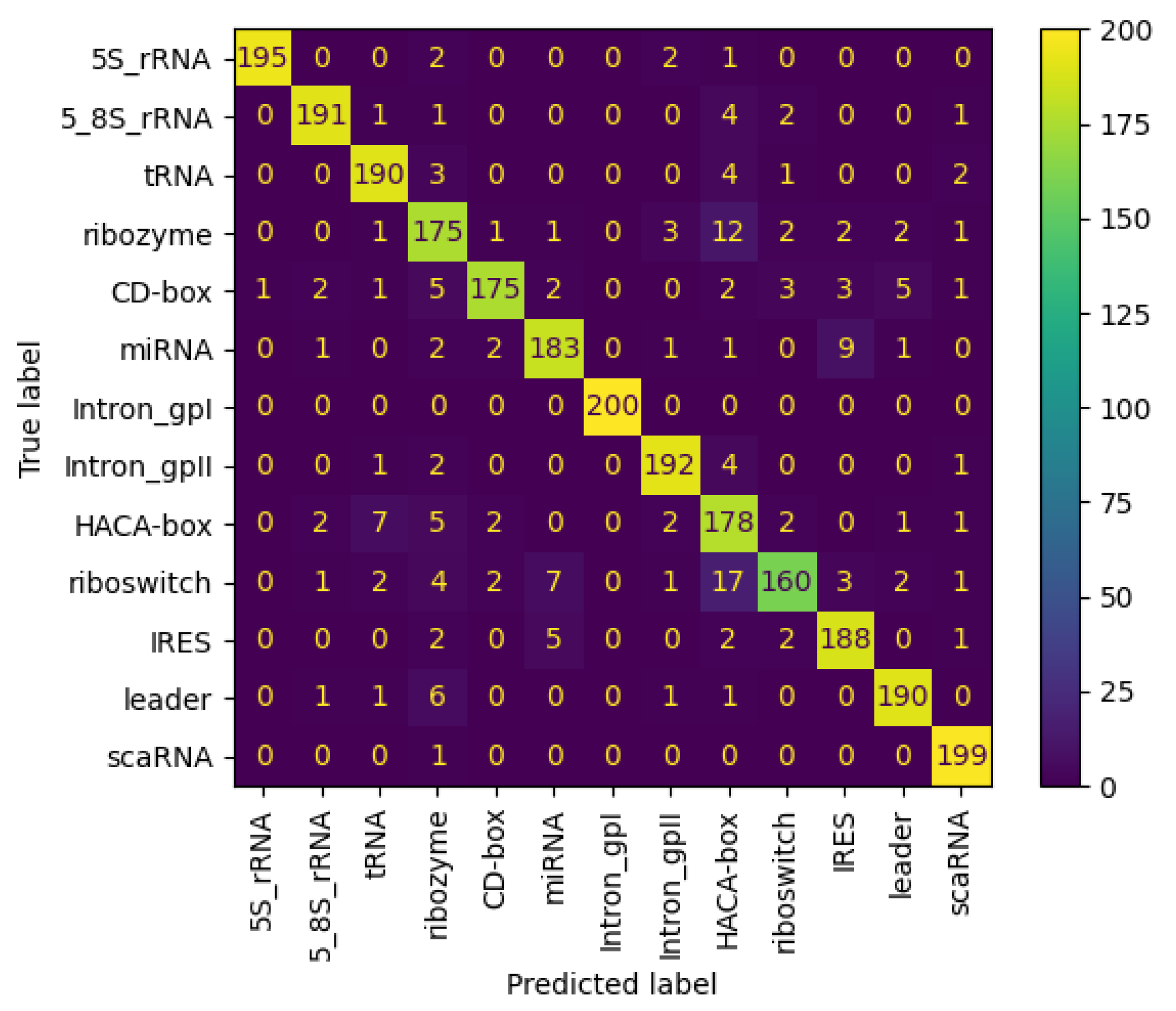
3.6.2. Results on NCC Dataset

The initial step involved dividing the NCC dataset into training and testing sets. The model was trained using 35,427 sequences with the parameters shown in Table 5, while the remaining 17,450 were used for testing purposes. Table 6 shows the testing metrics using the NCC dataset with four- and eight-digit RNA base encoding. In both cases, the systems are very efficient, approaching almost perfectly the ground truth values.
Figure 11 and Figure 12 present the confusion matrices for the NCC dataset, respectively indicating the performance of the proposed NCC model on four-digit and eight-digit encoding. These matrices are useful for visually checking the model’s predictive accuracy by displaying true versus predicted labels for all classes. By analyzing these figures, the quality of discrimination between very similar classes can be assessed, and confusion patterns can be identified, indicating areas where the model may be further improved, including adjustments to the model architecture or training process. As observed, the matrices exhibit high values along the diagonal, indicating a strong rate of correct classifications, with only a small proportion of misclassifications appearing in off-diagonal elements.

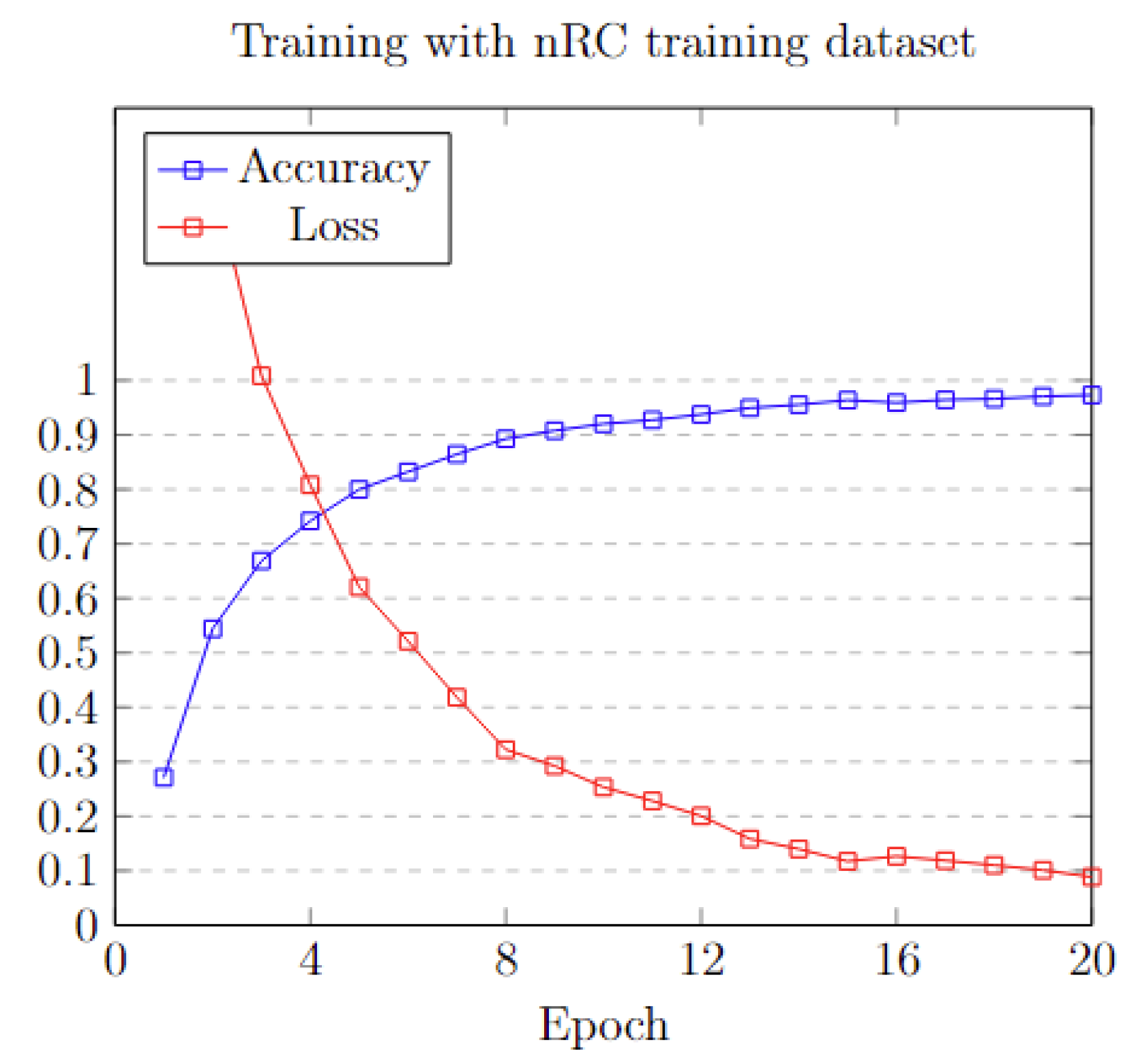
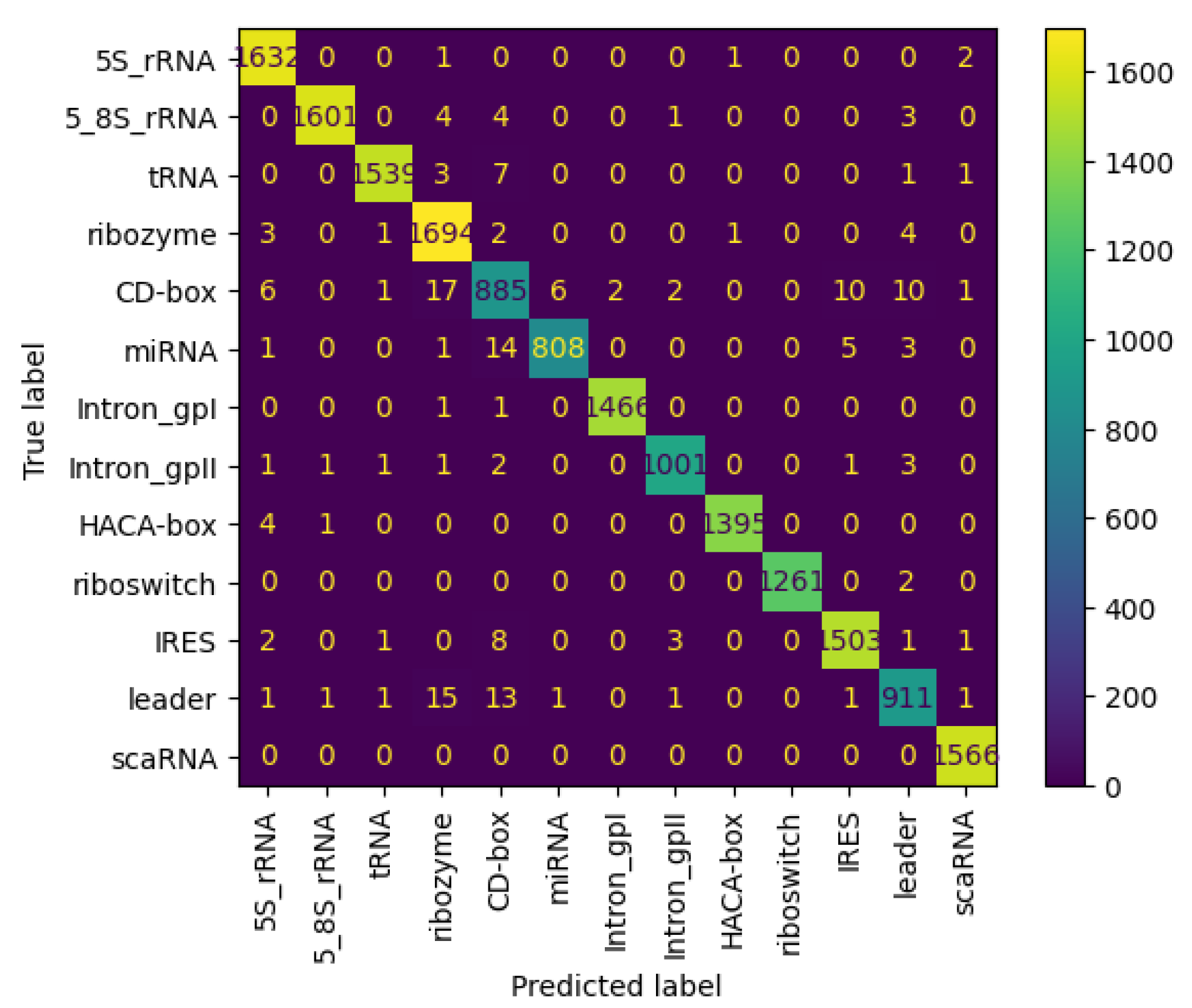
3.6.3. Results on nRC Dataset

To accurately assess the efficiency of the proposed NCC model, a comparison with state-of-the-art non-coding classifiers is presented. Training and testing the systems on the same dataset is crucial for a fair and precise comparison, ensuring that the results are directly comparable without data-variation influences. In this section, a comparative analysis of key metrics for the state-of-the-art classifiers is presented. In particular, the NCC model was not explicitly optimized for this dataset but was trained and fine-tuned using the NCC dataset created during this study to ensure an unbiased comparison. This approach allows for a thorough analysis of the NCC model’s prediction capability relative to existing non-coding RNA classification methodologies.
Table 7 displays the efficiency of the examined systems in five metrics. From this data, it can be concluded that the NCC tool surpasses the other systems in all metrics. Specifically, it shows a slight improvement in accuracy, outperforming the next-best model, ncDENSE, by approximately 0.06.
This demonstrates the NCC tool’s superior capability in accurately classifying non-coding RNA sequences. Additionally, Figure 13 shows the confusion matrix for the nRC dataset, in regards to the proposed NCC model.

4. Conclusions and Future Work

This work focuses on the development and evaluation of a tool designed to classify ncRNAs, aiming to enhance our knowledge of the functions of RNA and the role of ncRNAs in various chemical processes. An illustrative aspect of the research is the creation of a new dataset, the NCC dataset, which is wider than the nRC previously utilized by ten times, providing a robust foundation for preparing a machine learning-based classifier. The research involves a comprehensive examination of the NCC and nRC sets, which reveals the inherent complexity of ncRNAs. A significant contribution of this research is the creation of a novel deep learning model, called NCC, specifically adjusted for the classification of ncRNA. It uniquely encodes RNA sequences directly, thereby avoiding potential inaccuracies associated with RNA secondary structure prediction tools. The proposed model has shown the highest prediction capability, marginally surpassing state-of-the-art systems in accuracy, tested on the same dataset. In particular, the model achieved accuracy rates as high as 98% with the larger created dataset, indicating substantial improvements in this challenging classification task. The findings highlight the effectiveness of the model and the advances made, while also addressing the current limitations of RNA databases, noting their underdevelopment and significant imbalance among RNA classes, with specific classes being underrepresented. This imbalance underscores the ongoing need for more sophisticated and precise methodologies in the field of ncRNA classification. Active research and interest in this area suggest that future developments will likely bring about new methodologies that will further improve classification capabilities.
Although the NCC model did not take advantage of secondary structure and graph properties, their potential significance should not be overlooked. While these structures and their information were not utilized in the proposed model, they may provide essential knowledge and improve the model’s prediction capability. Investigating their incorporation into future versions may reveal hidden patterns and other notable discoveries in the data, potentially resulting in more robust classifications. Given their importance within the wider scope of the field, further investigation and consideration of these factors are warranted.

Author Contributions

Conceptualization, K.V. and I.M.; methodology, K.V. and I.M.; software, K.V.; validation, C.P. and E.M.; formal analysis, C.P. and E.M.; writing—original draft preparation, C.P. and E.M.; writing—review and editing, E.M. and C.P.; visualization, K.V.; supervision, C.P. and I.M.; project administration, I.M. All authors have read and agreed to the published version of the manuscript.

Funding

This research received no external funding.

Institutional Review Board Statement

Not applicable.

Informed Consent Statement

Not applicable.

Data Availability Statement

Data are contained within the article.

Conflicts of Interest

The authors declare no conflicts of interest.

References

  1. Hüttenhofer, A.; Vogel, J. Experimental approaches to identify non-coding RNAs. Nucleic Acids Res. 2006, 34, 635–646. [Google Scholar] [CrossRef] [PubMed]
  2. Feng, D.F.; Doolittle, R.F. Progressive sequence alignment as a prerequisitetto correct phylogenetic trees. J. Mol. Evol. 1987, 25, 351–360. [Google Scholar] [CrossRef] [PubMed]
  3. NCC: Non-Coding RNA Classifier. Available online: https://github.com/vassilas/NCC (accessed on 24 April 2025).
  4. Mattick, J.; Makunin, I. Non-coding RNA. Hum. Mol. Genet. 2006, 15, R17–R29. [Google Scholar] [CrossRef]
  5. Griffiths-Jones, S.; Bateman, A.; Marshall, M.; Khanna, A.; Eddy, S. Rfam: An RNA family database. Nucleic Acids Res. 2003, 31, 439–441. [Google Scholar] [CrossRef]
  6. RNAcentral Consortium. RNAcentral 2021: Secondary structure integration, improved sequence search and new member databases. Nucleic Acids Res. 2020, 49, D212–D220. [Google Scholar] [CrossRef]
  7. Kalvari, I.; Argasinska, J.; Quinones-Olvera, N.; Nawrocki, E.; Rivas, E.; Eddy, S.; Bateman, A.; Finn, R.; Petrov, A. Rfam 13.0: Shifting to a genome-centric resource for non-coding RNA families. Nucleic Acids Res. 2017, 46, D335–D342. [Google Scholar] [CrossRef] [PubMed]
  8. Andrikos, C.; Makris, E.; Kolaitis, A.; Rassias, G.; Pavlatos, C.; Tsanakas, P. Knotify: An Efficient Parallel Platform for RNA Pseudoknot Prediction Using Syntactic Pattern Recognition. Methods Protoc. 2022, 5, 14. [Google Scholar] [CrossRef]
  9. Makris, E.; Kolaitis, A.; Andrikos, C.; Moulos, V.; Tsanakas, P.; Pavlatos, C. Knotify+: Toward the Prediction of RNA H-Type Pseudoknots, Including Bulges and Internal Loops. Biomolecules 2023, 13, 308. [Google Scholar] [CrossRef]
  10. Koroulis, C.; Makris, E.; Kolaitis, A.; Tsanakas, P.; Pavlatos, C. Syntactic Pattern Recognition for the Prediction of L-Type Pseudoknots in RNA. Appl. Sci. 2023, 13, 5168. [Google Scholar] [CrossRef]
  11. Makris, E.; Kolaitis, A.; Andrikos, C.; Moulos, V.; Tsanakas, P.; Pavlatos, C. An Intelligent Grammar-Based Platform for RNA H-type Pseudoknot Prediction. In Artificial Intelligence Applications And Innovations. AIAI 2022 IFIP WG 12.5 International Workshops; Springer: Cham, Switzerland, 2022; pp. 174–186. [Google Scholar]
  12. Jabbari, H.; Wark, I.; Montemagno, C.; Will, S. Knotty: Efficient and accurate prediction of complex RNA pseudoknot structures. Bioinformatics 2018, 34, 3849–3856. [Google Scholar] [CrossRef]
  13. Sato, K.; Kato, Y.; Hamada, M.; Akutsu, T.; Asai, K. IPknot: Fast and accurate prediction of RNA secondary structures with pseudoknots using integer programming. Bioinformatics 2011, 27, i85–i93. [Google Scholar] [CrossRef] [PubMed]
  14. Ren, J.; Rastegari, B.; Condon, A.; Hoos, H.H. HotKnots: Heuristic prediction of RNA secondary structures including pseudoknots. RNA 2005, 11, 1494–1504. [Google Scholar] [CrossRef] [PubMed]
  15. Bellaousov, S.; Mathews, D.H. ProbKnot: Fast prediction of RNA secondary structure including pseudoknots. RNA 2010, 16, 1870–1880. [Google Scholar] [CrossRef] [PubMed]
  16. Panwar, B.; Arora, A.; Raghava, G. Prediction and classification of ncRNAs using structural information. BMC Genom. 2014, 15, 127. [Google Scholar] [CrossRef]
  17. Li, G.; Zhao, B.; Su, X.; Yang, Y.; Hu, P.; Zhou, X.; Hu, L. Discovering consensus regions for interpretable identification of RNA N6-methyladenosine modification sites via graph contrastive clustering. IEEE J. Biomed. Health Inform. 2024, 28, 2362–2372. [Google Scholar] [CrossRef]
  18. Qiu, S.; Liu, R.; Liang, Y. GR-m6A: Prediction of N6-methyladenosine sites in mammals with molecular graph and residual network. Comput. Biol. Med. 2023, 163, 107202. [Google Scholar] [CrossRef]
  19. Childs, L.; Nikoloski, Z.; May, P.; Walther, D. Identification and classification of ncRNA molecules using graph properties. Nucleic Acids Res. 2009, 37, e66. [Google Scholar] [CrossRef]
  20. Nithin, C.; Mukherjee, S.; Basak, J.; Bahadur, R. NCodR: A multi-class support vector machine classification to distinguish non-coding RNAs in Viridiplantae. Quant. Plant Biol. 2022, 3, e23. [Google Scholar] [CrossRef]
  21. Dunkel, H.; Wehrmann, H.; Jensen, L.R.; Kuss, A.W.; Simm, S. MncR: Late Integration Machine Learning Model for Classification of ncRNA Classes Using Sequence and Structural Encoding. Int. J. Mol. Sci. 2023, 24, 8884. [Google Scholar] [CrossRef]
  22. Wang, L.; Zheng, S.; Zhang, H.; Qiu, Z.; Zhong, X.; Liu, H.; Liu, Y. ncRFP: A Novel end-to-end Method for Non-Coding RNAs Family Prediction Based on Deep Learning. IEEE/ACM Trans. Comput. Biol. Bioinform. 2021, 18, 784–789. [Google Scholar] [CrossRef]
  23. Min, S.; Lee, B.; Yoon, S. Deep learning in bioinformatics. Briefings Bioinform. 2016, 18, 851–869. [Google Scholar] [CrossRef] [PubMed]
  24. Ji, Y.; Zhou, Z.; Liu, H.; Davuluri, R. DNABERT: Pre-trained Bidirectional Encoder Representations from Transformers model for DNA-language in genome. Bioinformatics 2021, 37, 2112–2120. [Google Scholar] [CrossRef] [PubMed]
  25. Hwang, Y.; Cornman, A.; Kellogg, E.; Ovchinnikov, S.; Girguis, P. Genomic language model predicts protein co-regulation and function. Nat. Commun. 2024, 15, 2880. [Google Scholar] [CrossRef] [PubMed]
  26. Fiannaca, A.; La Rosa, M.; La Paglia, L.; Rizzo, R.; Urso, A. nRC: Non-coding RNA Classifier based on structural features. BioData Min. 2017, 10, 27. [Google Scholar] [CrossRef]
  27. Wang, L.; Zhong, X.; Wang, S.; Liu, Y. ncDLRES: A novel method for non-coding RNAs family prediction based on dynamic LSTM and ResNet. BMC Bioinform. 2021, 22, 447. [Google Scholar] [CrossRef]
  28. Chen, K.; Zhu, X.; Hao, L.; Wang, J.; Liu, Z.; Liu, Y. ncDENSE: A novel computational method based on a deep learning framework for non-coding RNAs family prediction. BMC Genom. 2022, 24, 68. [Google Scholar] [CrossRef]
  29. Avila Santos, A.P.; de Almeida, B.L.S.; Bonidia, R.P.; Stadler, P.F.; Stefanic, P.; Mandic-Mulec, I.; Rocha, U.; Sanches, D.S.; de Carvalho, A.C.P.L.F. BioDeepfuse: A hybrid deep learning approach with integrated feature extraction techniques for enhanced non-coding RNA classification. RNA Biol. 2024, 21, 1–12. [Google Scholar] [CrossRef]
  30. Zhao, Q.; Zhao, Z.; Fan, X.; Yuan, Z.; Mao, Q.; Yao, Y. Review of machine learning methods for RNA secondary structure prediction. PLoS Comput. Biol. 2021, 17, e1009291. [Google Scholar] [CrossRef]
  31. Schuster, M.; Paliwal, K. Bidirectional recurrent neural networks. IEEE Trans. Signal Process. 1997, 45, 2673–2681. [Google Scholar] [CrossRef]
  32. Chollet, F. Others Keras. 2015. Available online: https://keras.io (accessed on 4 April 2025).
  33. Zhao, J.; Li, Y.; Wang, C.; Zhang, H.; Zhang, H.; Jiang, B.; Guo, X.; Song, X. IRESbase: A Comprehensive Database of Experimentally Validated Internal Ribosome Entry Sites. Genom. Proteom. Bioinform. 2020, 18, 129–139. [Google Scholar] [CrossRef]
  34. Fu, L.; Niu, B.; Zhu, Z.; Wu, S.; Li, W. CD-HIT: Accelerated for clustering the next-generation sequencing data. Bioinformatics 2012, 28, 3150–3152. [Google Scholar] [CrossRef] [PubMed]
  35. Kingma, D.; Ba, J. Adam: A Method for Stochastic Optimization. In Proceedings of the International Conference on Learning Representations, Banff, AB, Canada, 14–16 April 2014. [Google Scholar]
Figure 1. NCC dataset, RNA sequence length distribution.
Technologies 13 00196 g001
Figure 2. NCC neural network architecture.
Technologies 13 00196 g002
Figure 3. Sequences per class in NCC dataset.
Technologies 13 00196 g003
Figure 4. Length mean and STD, grouped by class and sorted by STD of NCC dataset.
Technologies 13 00196 g004
Figure 5. Sequence length distribution of miRNA (a) and ribozyme (b).
Technologies 13 00196 g005
Figure 6. Length mean and STD, grouped by class and sorted by STD of nRC dataset.
Technologies 13 00196 g006
Figure 7. Sequence length distribution of tRNA class in nRC (a) and NCC (b) datasets.
Technologies 13 00196 g007
Figure 8. Sequence length distribution of f ribozyme RNA class in nRC (a) and NCC (b) datasets.
Technologies 13 00196 g008
Figure 9. Sequence length distribution of leader RNA class in nRC (a) and NCC (b) datasets.
Technologies 13 00196 g009
Figure 10. Training accuracy and loss on each epoch.
Technologies 13 00196 g010
Figure 11. Confusion matrix of NCC model trained and tested with NCC dataset (4 digits).
Technologies 13 00196 g011
Figure 12. Confusion matrix of NCC model trained and tested with NCC dataset (8 digits).
Technologies 13 00196 g012
Figure 13. Confusion matrix of NCC model trained and tested with nRC dataset.
Technologies 13 00196 g013
Table 1. RNA IUPAC system’s encoding format.
IUPAC CodeMeaningComplementEncoding
AAT1000 0000 0000 0000
CCG0100 0000 0000 0000
GGC0010 0000 0000 0000
T/UTA0001 0000 0000 0000
MA or CK0000 1000 0000 0000
RA or GY0000 0100 0000 0000
WA or TW0000 0010 0000 0000
SC or GS0000 0001 0000 0000
YC or TR0000 0000 1000 0000
KG or TM0000 0000 0100 0000
VA or C or GB0000 0000 0010 0000
HA or C or TD0000 0000 0001 0000
DA or G or TH0000 0000 0000 1000
BC or G or TV0000 0000 0000 0100
NG or A or T or CN0000 0000 0000 0010
XNone-0000 0000 0000 0000
Table 2. RNA bases in one-hot encoding format.
Base4 Digits8 Digits
A10001000 0010
T/U01000100 0001
G00100010 1000
C00010001 0100
X00000000 0000
Table 3. Sequences grouped by family and database.
RNA FamilySource# of Sequences
IRESRfam1472
IRESIRESbase1328
leaderRfam31,662
riboswitchRfam69,465
miRNARfam387,173
ribozymeRfam220,007
CD-boxRfam132,915
HACA-boxRfam36,938
scaRNARfam2962
tRNARfam1,432,442
5S_rRNARfam140,644
5_8S_rRNARfam4940
Intron_gpIRfam2611
Intron_gpIIRfam15,729
Table 4. Sequences per family in NCC dataset.
RNA FamilyNumber of Sequences
IRES2800
leader3061
riboswitch3791
miRNA4317
ribozyme4630
CD-box4661
HACA-box4931
scaRNA2962
tRNA4882
5S_rRNA4882
5_8S_rRNA4940
Intron_gpI2611
Intron_gpII4409
Table 5. NCC model training parameters.
Number of epochs20/50/100
Batch size128
Steps per epochDefault = 277
OptimizerAdam
Loss functionCategorical Cross Entropy
Shuffle train dataTrue
Table 6. Results on the NCC dataset for the two proposed variations (4 and 8 digits).
One-Hot EncAccuracySensitivityPrecisionF-ScoreMCC
8 Digits0.989220.986510.987890.987180.98828
4 Digits0.990540.988640.988860.988730.98971
Table 7. Model comparison.
Model/MethodAccuracySensitivityPrecisionF-ScoreMCC
RNAcon0.37370.37870.45000.36050.3341
GraPPLE0.64870.66840.73250.70500.6857
nRC0.69600.68890.68780.68780.6627
ncRFP0.79720.78780.79040.78830.7714
ncDLRES0.84300.83440.84190.84070.8335
ncDENSE0.86870.86770.87030.86670.8574
NCC 4d0.92690.92690.92860.92680.9210
NCC 8d0.92920.92920.93110.92930.9234
Disclaimer/Publisher’s Note: The statements, opinions and data contained in all publications are solely those of the individual author(s) and contributor(s) and not of MDPI and/or the editor(s). MDPI and/or the editor(s) disclaim responsibility for any injury to people or property resulting from any ideas, methods, instructions or products referred to in the content.

