Abstract
In recent decades, missile guidance and control have advanced significantly, with methods like pure pursuit (PP), command to line-of-sight (CLOS), and proportional navigation (PN) enabling accurate target interception in uncertain environments through line-of-sight (LOS) tracking. In this work, we propose a novel 3D sliding pure pursuit guidance (3DSPP) law for controlling a surface-to-air missile against a maneuvering target. The algorithm is compared with established guidance laws such as zero-effort miss distance “ZEM-PN” and “3D-PP”, with performance metrics including the miss distance and time of closest approach . The results demonstrate that the 3DSPP outperforms the conventional methods by achieving the lowest 0.1497 m and the fastest 7.3853 s, ensuring more precise and rapid interception. The algorithm also exhibits superior robustness to noise and efficient energy management, making it a promising solution for real-world missile guidance systems.
1. Introduction
Driving the purser to intercept a specific target with zero miss distance is the primary goal of missile guidance laws, and in this regard, it can be said that the missile is trying to hit the target in a stable manner and with high accuracy [1]. However, this is rarely possible, as there is always a miss distance between the target and the point where the missile explodes. Therefore, the goal of missile control is to reduce the miss distance to avoid hitting the wrong target and to ensure that the maximum damage is inflicted on the intended target [2]. One of the most practical laws of missile guidance is the Proportional Navigation Guidance (PNG) law, which has been proven to be an effective and simple guidance algorithm for homing guidance systems, thus showing its wide applications over the past few decades [3,4]. The main principle of PNG is to apply a lateral acceleration command to nullify the line-of-sight (LOS) rate, thereby forcing the interceptor to remain within the collision triangle. The LOS angular rate information needed in the guidance law can be obtained by an onboard seeker. To improve the miss distance performance of guided missiles, several techniques have been proposed. The optimization of the PNG algorithm was studied in a paper [5], and its extension to the 3D scenario can be found in [6,7]. The most common forms of proportional navigation (PN) include true PN, where acceleration is directed perpendicular to the line of sight; pure PN, where acceleration is directed perpendicular to the interceptor’s velocity vector; and ideal PN, where acceleration is directed perpendicular to the relative velocity vector. However, certain other forms are based on differential geometry [8]. In recent years, extensive research has been devoted to the field of homing guidance systems, largely due to their capability to achieve “fire-and-forget” attacks. With the advancement of nonlinear control theory, a significant number of terminal guidance laws related to homing guidance have been proposed, such as the Multi-Task Switching Guidance [9,10], Integrated Guidance and Control Design [11], Deep Reinforcement Learning-Based Intelligent Guidance [12], Path-Following Approach [13], Cooperative guidance of seeker-less missile [14], Fuzzy and Sliding Mode-based Guidance [15], The modified 3D-PN navigation has been extensively discussed in the literature for over half a century [16]. When considering target interception alone, the tracking error is defined as either the zero-effort miss (ZEM) distance or the LOS rate. Nullifying one of them results in a perfect interception [17].
Numerous missile guidance and control laws have been developed over the years, ranging from classical linear designs to more advanced modern systems. Among these, the most widely used guidance law is a form of proportional navigation. Autonomous missiles employing some variant of the PN guidance law require the measurement of the line-of-sight (LOS) angle rate and the estimation of closing or missile velocity. This implies that the missile seeker is capable of detecting and tracking targets during engagement [18]. Most analytical studies on missile guidance problems in two-dimensional engagements assume that the missile follows the proportional guidance command. Researchers then attempt to solve a system of coupled nonlinear ordinary differential equations or apply optimal control methods to devise different guidance commands. In three-dimensional engagements, Bezick employs classical differential geometry to explore missile guidance problems and derives the proportional navigation law based on geometric curvature [19]. Some people apply optimal control techniques to design feedback guidance laws [20,21]. Some other researchers explore the practicalities of realistic true proportional navigation (RTPN) problems [22]. Furthermore, Yang Ciann D extracts analytical solutions for missiles following the generalized proportional navigation guidance commands using elliptical functions. Zhibing Li has developed the Field-to-View Constrained Integrated Guidance [23]. In this review, the following fundamental guidance schemes were discussed: command to line of sight, beam riding, pursuit guidance, proportional navigation, and ZEM-PN guidance. The first two guidance laws cannot be used for “fire-and-forget” weapons due to the requirement for continuous target tracking with an external tracker. However, the other three systems {pure pursuit, PN, and ZEM-PN} can be used for “fire-and-forget” weapons. From an operational standpoint, having a “fire-and-forget” weapon is desirable, which necessitates a seeker sensor. It is relatively easy to use proportional navigation or ZEM-PN guidance laws with spinning seekers; however, spinning seekers are expensive [24].
The conceptual idea behind pure pursuit guidance is that the missile should always head for the target’s current position [25,26]. Provided that the missile’s velocity is greater than the target’s, this strategy will result in an intercept. The required information for velocity pursuit is limited to the bearing to the target, which can be obtained from a simple seeker, and the direction of the missile’s velocity [27]. In the early days, pure pursuit was implemented in laser-guided missiles, where a simple seeker is mounted on a vane, which automatically aligns with the missile’s velocity vector relative to the wind. The mission of the guidance and control system thus is to steer the missile such that the target is centered in the seeker [28]. The pure pursuit guidance law results in highly demanded lateral acceleration, in most cases infinite at the final phase of the intercept. As the missile cannot perform infinite acceleration, the result is a finite miss distance. Pure pursuit is thus sensitive to the target velocity and to disturbances such as wind. The most important writers who have written on direct pursuit navigation guidance are listed below. Among the key contributors to the field of direct pursuit navigation guidance are the following authors: Malafeyev Oleg discussed the pursuit problem for unmanned aerial vehicles [29]; Yaoyu Sui proposed a fuzzy pure pursuit method for autonomous UGVs [30]; Zitao Su focused on evading an unknown pursuer through pursuit strategy identification [31]; Zhihan Li researched the head pursuit interception strategy for hypersonic targets [32]; Shneydor N.A. examined missile guidance and pursuit [33]; Tal Shima contributed to the field in 2011 [34]; Takeshi Yamasaki studied sliding mode-based pure pursuit guidance [35]; and, finally, Kumar S.R. investigated deviated pursuit strategies [36]. The classical pursuit guidance law is not suitable for meter precision [37]. Despite all of this, most of the “smart weapons” (bombs and missiles) that were used extensively in the latest wars utilized the PP geometrical rule, homing on laser-illuminated ground targets. More recently, smart bullets based on the same principles have also been proposed [38]. Our motivation is to transfer this technology for use in surface-to-air missiles, aiming for high accuracy and performance. While it has often been claimed that the technology is sensitive to fast-moving targets, we demonstrate that the proposed method, known as 3D pure pursuit guidance, offers significant robustness against disturbances and low sensitivity to target velocity.
This paper begins with the introduction of a dynamic model for a 6DOF generic missile. In Section 3, we present the autopilot model and control system. Section 4 provides an overview of existing guidance laws. In Section 5, we propose a novel guidance law, referred to as 3D pure pursuit, along with an enhanced version “3D sliding pursuit guidance”. To optimize the guidance performance, we employ the Particle Swarm Optimization (PSO) technique. Section 6 validates the effectiveness of the proposed method by presenting numerical results that demonstrate its improved performance. The paper concludes with a summary of the findings. This work is motivated by the fact that, to the best of the authors’ knowledge, no previous research has addressed a similar algorithm.
2. Dynamic Models of Generic Missiles
This subsection outlines the development of a nonlinear model for a missile with a variable mass, accounting for fuel consumption during flight. It improves the accuracy of performance predictions by reflecting the dynamic changes in mass.
2.1. Six-Degree-of-Freedom Variable Mass Non-Linear Model
Missile models employ math equations to describe their dynamics based on applied forces and moments. Using equations of motion, the 6-DOF movement is defined by the translation of the center of mass and 3-DOF rotation around it. Inputs include forces and moments, while outputs are the resulting accelerations (U.S.A Missile Command) [39]. For a space-rotating continuum rigid body, the relation holds for each point in the rigid body, where is the position vector of the center of mass “radial from the rotation axis”, is the angular velocity, and is the tangential velocity. If is a rotation matrix that rotates to be and we define the tensor of rotation , then
where is a vector formed by skew-symmetric tensor , and . So, it is always valid that .
Consider a fixed system , assumed to be the inertial frame, and another rotating system , assumed to be the body’s fixed frame, which rotates concerning the first one by an angular velocity . Let , , and be unit vectors along the axes of the rotating system. Let be an arbitrary vector with components , , and along the rotating axes. The relative accelerations are related by [40]
So, we deduce that (i.e., for both linear and angular velocities)
Mathematically, Newton’s second law can be expressed in terms of conservation of both linear and angular momentum by the following vector equations [41]:
where is the position vector. is the linear velocity vector in the body-fixed frame. is the angular velocity vector. is the angular momentum. is the moment act on the body. is the force acting on the body. is the moments of inertia about the frame axes. is the total mass of the missile (function of time). is the centripetal acceleration (see Appendix A).
In a decomposed form, the vectors of total forces and total moments can be rewritten as and , where is the missile weight and is the moment due to gravity. are the aerodynamic force and moment. is the propulsive force. is the moment vector thrust (i.e., propulsive moment). is the jet nozzle exit area. is the mass rate of flow of the exhaust gases. is the ambient atmospheric pressure. is the average pressure across . is the unit vector in the direction of the relative exhaust velocity. is the velocity of exhaust gas relative to the center of the missile.
Now, using the fact that and
and based on the assumption of symmetrical geometry of the missile, we obtain the product of inertia , and the above equation can be simplified more, as follows (see [42,43]):
2.2. The Euler Angles and the Navigation Model
We now aim to express the angular velocity of the rotating frame in terms of rotation angles (or Euler angles). Because the two reference frames (Earth–body) are rotating relative to each other, the direction matrix is a function of time.
The rotation matrix (or direction cosine matrix) is necessary to transform vectors/points from the body-fixed frame to the navigation reference frame and vice versa: for positive sense or for negative sense. In this study, we consider the negative rotation. Let us assume that is a position vector of an object in the body-fixed frame (i.e., independent of time). So, if we use the fact that and we take the derivative of with respect to time, then
On the other side, we know that
So, by the chain rule, we have
After simplification, we obtain
Hence, we obtain the Euler model
The navigation model (as detailed by Rafael Yanushevsky) can be obtained using the equation [43,44]
In the body-fixed frame, the missile speed is given by . The components u, v, and w can be written in terms of the vehicle speed , angle of attack , and the side slip angle as . Thus, we have to write where . The angle of attack is the angle between the horizontal and the segment connecting the two ends of the wing. The angle is the side slip angle. To simplify the calculations, the total angle of attack is sometimes defined as .
2.3. Propulsive and Aerodynamic Models
The value of the missile mass is the value determined by a table lookup as a function of the current simulation time, or, as an alternative, can be calculated within the simulation using the impulse-momentum theorem [38]
is the instantaneous mass of missile, . is the missile mass at the time of launch, . is the ref-thrust force (at sea level) and is the specific impulse of propellant . The discrete form of the above mass equation is given by .
The input thrust table is used to look up the thrust corresponding to the reference atmospheric pressure as a function of time. The thrust is corrected for the ambient atmospheric pressure by [45]
is the ambient atmospheric pressure, , and is the reference ambient pressure, .
Assuming that the moment of inertia varies linearly with the mass, the moment of inertia is updated using , where is the moment of inertia at launch, is the moment of inertia at burnout, is the instantaneous moment of inertia, and missile mass at burnout, .
The location of the center of mass varies linearly with the mass [42]: where is the instantaneous distance from nose to center of mass, is the distance at launch, is the distance at burnout, and simulated time, ( is the burnout time).
In most missiles, the magnitude of the thrust , is directed along the -axis (the missile centerline). Then, the components of the thrust vector expressed in the body reference frame are [40]: .
The thrust moment vector is given by , where is the distance from the missile nose to the current value .
The gravitational force expressed in body coordinates is calculated by multiplying by the matrix that transforms from earth to the body frame [46]:
The resultant (total) aerodynamic force on the missile can be resolved in any frame to give three orthogonal components [43]:
Since the drag force is by definition directed opposite the velocity vector and lift is by definition perpendicular to the velocity vector and lies in the plane formed by the velocity vector and the normal force vector, the aerodynamic force is given by
Equations for calculating the aerodynamic forces and moments affecting the missile are given by (Bureau of Naval Personnel)
where is the magnitude of aerodynamic drag force vector . is the magnitude of aerodynamic lift force vector . are components of in the body frame. are the aerodynamic drag, and lift, coefficients, . is the aerodynamic roll moment coefficient about the center of mass. is the aerodynamic pitch moment coefficient about the center of mass. is the aerodynamic yaw moment coefficient about the center of mass. is the aerodynamic reference area, . is the standard atmospheric density at sea level, . is the aerodynamic reference length of the body, . is the speed of the body, speed of air relative to the body, the magnitude of the velocity vector , .
The aerodynamic coefficients are given by the following equations [39,43]:
where is the zero-lift drag coefficient. is the slope of curve formed by versus . is the roll damping derivative. is the slope of the curve formed by versus . is a constant depending on the body shape and flow regime. are angles of effective control surface deflections. is the pitching moment coefficient about the reference station. is the yawing moment coefficient about the reference station. is a coefficient corresponding to the normal force on the -axis. is a coefficient corresponding to the normal force on the -axis. is the yaw damping derivative relative to yaw rate . is the yaw damping derivative relative to the rate of . is the pitch damping derivative relative to the pitch rate . is the pitch damping derivative relative to . is the instantaneous distance from the nose to the center of mass. is the distance from the nose to the reference moment station.
The pitch and yaw components of the aerodynamic moment about the moment reference station are calculated using , where is the slope of curve formed by versus . is the slope of the curve formed by versus . is the slope of the curve formed by versus and is the slope of the curve formed by versus . Since the studies missile is assumed to have cruciform symmetry, , , , and . Coefficients corresponding to the components of the normal force in the - and -axes are calculated by and , where is the dynamic pressure, and is the aerodynamic reference area, . is the atmospheric pressure, . The Mach number is given by , where is the speed of sound. Force coefficients are functions of the Reynolds number . Here, is the aerodynamic reference length (typically represents the missile’s diameter), is the body speed, is the atmospheric dynamic viscosity, and is the atmospheric density.
2.4. The Atmospheric Model
In applications in which measured atmospheric data are available at a few altitudes , the atmosphere in flight simulations is modeled using equations that extrapolate/interpolate data based on known atmospheric variation with altitude [45]. These equations are
where is the lapse rate, . is the atmospheric density, . is the magnitude of at earth surface , . is the altitude above sea level, . is the ref-altitude (sea level or earth surface), . is the pressure at altitude , . is the given pressure at altitude , . is the gas constant (287.05), . is the temperature at altitude , , and is the given temperature at altitude , . is the speed of sound at altitude , , and is the ratio of specific heat, . Some authors use the model (which is the approximate version of the previous one) .
Now, we present a schematic diagram that collects all the subsystems (see Figure 1).
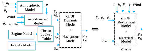
Figure 1.
Block diagram of the missile’s subsystems.
2.5. The Missile/Target Motion
In general, the equations of motion that describe the flight of a missile are equally applicable to an airborne target; however, the equations used to calculate target motion in a missile flight simulation are usually greatly simplified. Here, we are interested only in the kinematic model. The target position is updated using the following equation (see [40]):
is the total acceleration vector of the target, . is the position vector of target, , and is the velocity vector of target center of mass, . The function indicates that the variable is at the current time, . indicates that the variable was at a previous time. computation time step, .
The target acceleration vector is calculated using , where is the angular rate vector of the target flight path, . The weaving flight path can be modeled as a cosine curve: , where is the max-maneuver acceleration. is the commanded target maneuver acceleration. is the period of target wave maneuver, , and is the time since starting the maneuver, . To avoid the discontinuities in the commanded target acceleration, we pass through a first-order transfer function (low-pass filter) before using it in a digital simulation [41]. The following steps summarize the curved path for target maneuver:
Diff-equations of missile velocity yield the components of the missile position vector in the Earth coordinates with . The relative range vector extends from the missile’s center of mass to the target’s center of mass, aligning with the line-of-sight vector if the distances from the missile’s seeker and the track point are negligible. It is calculated in the Earth frame as , where and are the position vectors of the missile and target, respectively. The relative velocity vector is the difference between the target and missile velocities: , representing the target’s velocity relative to the missile. Normalizing this relative vector gives the unit vector , indicating the direction of . The miss distance is often used as a measure of missile system performance (see Figure 2). In general, the smaller the miss distance, the greater the probability of killing the target. The missile kill probability is a function of many factors, including the fuse, warhead characteristics, and target vulnerability [2,8]. An acceptable (sufficiently small) is the first criterion of a successful engagement.
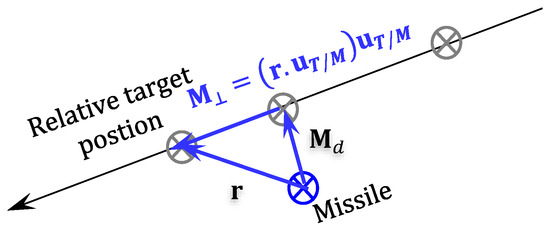
Figure 2.
Representation of the miss distance vector diagram.
3. Autopilot Model and Control
3.1. Different Types of Homing Guidance
A guidance system is called homing (see all types in Figure 3) if the missile detects the target and tracks it thanks to the energy emitted by the latter. If the source of the energy is the target , e.g., radio transmissions, acoustic noise, or heat, the homing is called passive. If reflects energy beamed at it by , then this is active homing. In semi-active systems, homes onto energy reflected by , the latter being “illuminated” by a source I external to both (see [19,33,47]). The expression homing guidance is used to describe a missile system that can sense the target by some means and then guide itself to the target by sending commands to its own control surfaces. Homing is useful in tactical missiles where considerations such as autonomous operation usually require sensing of the target motion to be performed from the interceptor (pursuer) itself [48].
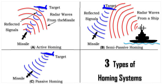
Figure 3.
Block diagram of different types of homing systems (passive, semi-passive, and active).
3.2. The Autopilot and the Control Systems
The autopilot is a link between the function that indicates a change of heading is needed (guidance processor) and the mechanism that can change the heading (control system). The “autopilot” receives guidance commands and processes them to the controls such as deflections or rates of deflection of control surfaces or jet controls. The control subsystem transfers the autopilot commands to aerodynamic or jet control forces and moments to change the position of the airframe and to attain the commanded maneuver by rotating the body of a missile to a desired angle of attack [42] (see Figure 4). The design of the autopilot depends on the aerodynamics and the type of controls employed.
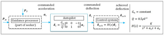
Figure 4.
Block diagram of the autopilot function.
3.3. The Deflection Commands
Autopilot in a missile has two basic functions: to ensure stable flight and to translate the guidance law into control-surface deflection commands (Figure 5). It is assumed that the studied missile has four control surfaces in a cruciform pattern and that commanded control-surface deflections are proportional to commanded lateral accelerations for maneuver commands and proportional to commanded roll rates for roll commands. In the six-degree-of-freedom model, the pitch and yaw channels can be considered as decoupled SISO systems; this simplifies their design. A constant roll position creates normal working conditions for missile components.
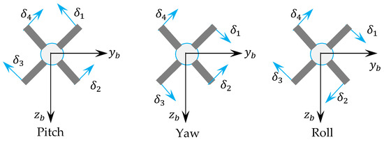
Figure 5.
Convention for the direction of control-surface rotation.
The relationship between the actuator commands and the individual fin deflections is given for this model as , , and , where the deflection is the autopilot pitch fin command, is the autopilot yaw fin command, and is the autopilot roll fin command. is the deflection angle of the control surface, i = 1, 2, 3, 4. In the five-degree-of-freedom (5DOF) model, the pitch and yaw channels are coupled and the roll rate is set to zero; thus, the actuator commands are . The restrictions related to the fin deflections are transformed into the autopilot limits , which, in turn, impose constraints on missile acceleration [40,43].
3.4. Commanded Signals
The designs of the control system actuators of diff-missiles may vary considerably, but all have a common purpose, i.e., to convert autopilot commands into fin deflections. The input to the model is the control-surface deflection command; the output is the control-surface defection achieved. The commanded lateral acceleration vector is an essential design parameter and is computed by one type of known guidance control law, such as the LOS (or beam rider) control or proportional navigation control. The vector is transformed to the body ref-frame by . The actuator piston pressure for control surfaces 1 and 2 are given by and , where is the actuator pressure for the pitch channel and is the actuator pressure for the yaw channel. is the gain factor relating the actuator pressure to acceleration command . For a given actuator pressure , then the actuator hinge moment is , where is the actuator piston area and is the bell crank lever arm. The hinge moment is balanced by an aerodynamic moment on the control surface about the hinge axis, given by , where is a surface aerodynamic coefficient derivative, is the aerodynamic reference length of the control surface, is the reference surface area, and is the control-surface angle of attack. The angle of attack that causes the two moments to be balanced is determined by equating the moments and solving for (i.e., ). If we define the constant and combine those equations, we can derive the control-surface angles of attack. The control-surface angles of attack that result from the actuator pressures commanded by autopilot are given by and , where is a gain factor relating the angle of attack to acceleration command per unit dynamic pressure . is the commanded angle of attack of the pitch-channel control surface. is the commanded of yaw-channel control surface [39]. The direct relationship between the commanded accelerations and the commanded deflections can be captured by the matrix equation , where is the autopilot gain matrix and is the commanded deflections . When , then the actual missile roll rate is known to be small enough to have a negligible effect on the missile guidance and dynamics, and so the rotation model can be simplified considerably by setting . Simplifications are sometimes made in the missile model by approximating or neglecting altogether the degree of freedom that represents missile roll; this results in a 5-DOF model. In such case, the roll deflection is negligible.
Note: In some simulations, the roll of the missile is not explicitly taken into account, or it can be calculated by other means and thus eliminates the need for the body axes to roll with the missile. In these applications, the body coordinate system translates, yaws, and pitches with the missile but does not roll. If the missile roll rate is rapid enough to affect missile performance significantly, six degrees of freedom may be required.
To clarify things more, an illustration is shown in Figure 6 that presents the cascade function of the three essential parts of missile control.
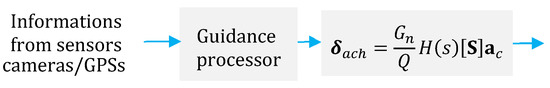
Figure 6.
Functional Architecture of Missile Control: Guidance, Autopilot, and Control System.
and is the transfer function of the linear servomechanism.
3.5. Signal Processing and Data Filtering
The seeker LOS vector is assumed to be identical with the range vector . The angular rate of the seeker head lags the angular rate of the line-of-sight vector. This lag is taken into account when calculating the guidance commands. This lag is assumed to be represented by a first-order transfer function, and the seeker-head rate is calculated by
There are assumed to be delays involved in processing the seeker head angular rate signal. The filtered seeker head angular rate signal is given by the following relation:
where
- is the seeker tracking loop constant.
- is the seeker signal processing time constant.
The dynamic response of the autopilot–control system is described by a first-order system with time constant . The achieved angles of attack of the fins will lag those given in and as given by
is the achieved angle of attack of pitch channel control surface . is the achieved angle of attack of yaw channel control surface . The fin angles of incidence are calculated using the equations and . The absolute values of and are tested against the maximum fin deflection angle ; if the absolute value of a fin angle of incidence exceeds , it is reset to and retains its original sign (see [43,46]).
3.6. Servo System Modeling
The designs of the control system components—power sources, power transmission media, servos, and actuators of different missiles—may vary considerably, but all have a common purpose, i.e., to convert autopilot commands into fin deflections [49]. The input to the closed loop servo system is the control-surface deflection command; the output is the control-surface defection achieved. The relationship between the output and the input is defined mathematically by appropriate transfer functions and logical elements, such as limits on the magnitudes of control-surface defections (Figure 7).
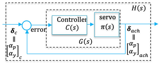
Figure 7.
Block diagram of the used servo system.
Generally, the servomotors are modeled by the first-order transfer function given by . The closed-loop transfer function is given by , where is the control system time constant depending on the type of motors and is some proportionality constant. Figure 8 illustrates the missile guidance and control loop depicting the interaction between the guidance system, control laws, and the missile’s dynamics. This closed-loop system ensures that the missile follows the desired trajectory to intercept the target effectively.
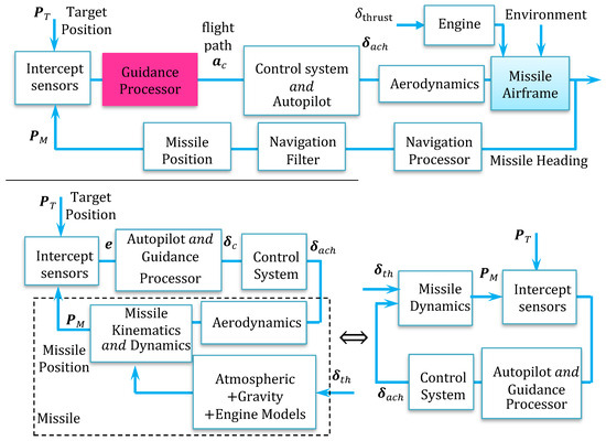
Figure 8.
The guidance, navigation, and control loops (an overview of missile flight control).
In control systems for aircraft and missiles, a limiter is often used between the servo (or actuator) model and the aerodynamic model to ensure that the control-surface deflections remain within physically feasible and aerodynamically safe limits. Using a limiter between the servo and aerodynamic model ensures that the deflections fed into the aerodynamic model are within safe, effective, and physically realizable limits. This prevents damage, ensures accurate modeling of the missile’s response, maintains stability, and ensures safety during operation. , where the limiter (or the clamp) function is written as
4. Overview of the Existing Guidance Laws
Guidance can be defined as the strategy for how to steer the missile to intercept, while control can be defined as the tactics of using the missile control actuators to implement the strategy. The most fundamental, most commonly used, guidance laws are as follows:
- Pure pursuit (and velocity pursuit);
- Proportional navigation and all of its variations;
- Command-to-line-of-sight and beam riding.
There are many other types of target interception, but here we explain graphically a few of them (Figure 9), namely, true pure pursuit, deviated pursuit, and the PN navigation.
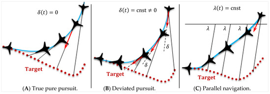
Figure 9.
Graphical representations of the different types of target interception guidance.
is the deviation angle between the line of sight and the interceptor’s velocity vector and is the angle of LOS to the reference line. All of these guidance laws date back to the first guided missiles developed in the 1940s–1950s. The reasons that they have been so successful are mainly that they are simple to implement and that they give robust performance. Before proceeding to the development of the proposed algorithm, we highlight some well-established guidance laws, as presented in [1,39,40]. These include the PN navigation, beam rider guidance, and the zero-effort-miss guidance law.
4.1. Proportional Navigation
Proportional navigation is the most widely known and used guidance law for short- to medium-range homing missiles because of its inherent simplicity and ease of implementation. Proportional navigation is so robust, however, that acceptable miss distances can be achieved even against targets that perform relatively severe evasive maneuvers if the missile response time is short enough and if the missile is capable of sufficient acceleration in a lateral maneuver [6,18]. The parallel navigation rule stats that the direction of the line of sight (LOS) is kept constant relative to inertial space, i.e., the LOS is kept parallel to the initial LOS. Proportional navigation (PN) is the guidance law that implements parallel navigation, but it kept the line-of-sight rate to be zero rather than of constant direction (see Figure 10). Therefore, in PN, the line of sight may change direction but with a zero rate. PN dictates that the missile velocity vector should rotate at a rate proportional to the rotation rate of the line of sight (LOS rate), and in the same direction (see [49,50]).
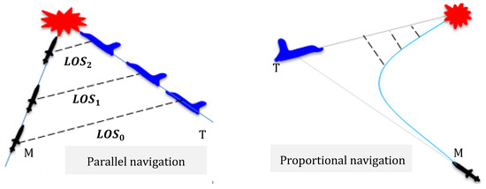
Figure 10.
PN guidance implements parallel navigation.
The main idea behind proportional navigation is that at the end of the course, the missile should keep a constant bearing on the target at all times (see Figure 11). As most sailors know, this strategy will result eventually in inevitable collision. The guidance law that is used to implement this concept is , where is the direction of the missile’s velocity vector, is the bearing of the missile to the target, and is a constant. Both and are measured relative to some fixed reference [6,22]. In mechanics, it is well-known that the normal acceleration is of the form . In light of this rule, it can be established that the commanded normal acceleration is given by
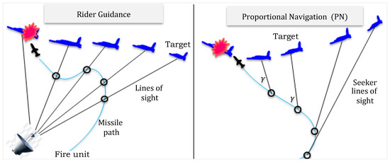
Figure 11.
Block diagram of beam rider guidance vs. proportional navigation guidance.
Here are some forms of the proportional guidance law.
Alternates of the Prop-Navigation guidance law are as follows:
where and .
For instance, in flying a proportional navigation course, the missile attempts to null out any line-of-sight rate that may be developing. The missile does this by commanding wing deflections to the control surfaces. Consequently, these deflections cause the missile to execute accelerations normal to its instantaneous velocity vector. Thus, the missile commands wing deflections to null out the measured rate [8,20]. A practical implementation of PN for RF seekers (see Figure 12) is obtained by calculating the commanded acceleration , where is the navigation constant (also known as navigation ratio, effective navigation ratio, and navigation gain), a positive real number; is the unit vector in the direction of centerline axis (from the tile to the nose of the missile); the missile centerline is given by the Euler angles as ; and is the filtered seeker-head angular rate signal .
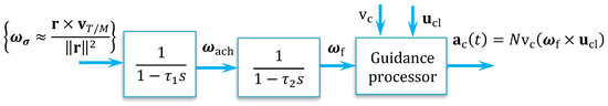
Figure 12.
Practical implementation of PN for RF seekers.
So, classical PN guidance is based on recognition of the fact that if two bodies are closing on each other, they will eventually intercept if the between the two does not rotate relative to the inertial space [10,12]. It is based on the fact that two vehicles are on a collision course when their direct does not change direction as the range closes.
4.2. Line of Sight (and/or Beam Rider) Guidance
A guided missile engagement is a highly dynamic process. The conditions that determine how close the missile comes to the target are continuously changing, sometimes at a very high rate. A guidance sensor measures one or more parameters of the path of the missile relative to the target. A logical process is needed to determine the required flight path corrections based on the sensor measurements. This logical process is called a guidance law. The objective of a guidance law is to cause the missile to come as close as possible to the target. Command-to-line-of-sight guidance is similar to beam rider guidance (see Figure 13) in that both forms attempt to keep the missile within a guidance beam transmitted from the ground. As shown in the figure, the vector represents the error in missile position relative to the guidance beam at any given instant. This error is defined as the perpendicular distance from the missile to the centerline of the guidance beam. Notice that the missile guidance commands generated by beam rider and command-to-line-of-sight systems are proportional to the error vector and the rate of change of that vector . The proportionality with causes the missile to be steered toward the center of the guidance beam; the proportionality with provides rate feedback, which causes the missile flight path to maneuver smoothly onto the centerline of the guidance beam without large overshoots.
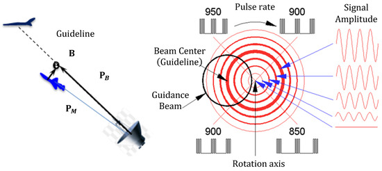
Figure 13.
Line of sight (and/or beam rider) guidance.
A third parameter, the Coriolis acceleration , may be included in the guidance equation. This Coriolis acceleration results from the angular rotation of the guidance beam. The Coriolis component of missile acceleration is required in order to allow the missile to keep up with the rotating beam as the missile flies out along the beam. In surface-to-air missile applications, the angular rate of the guidance beam is typically great enough to cause this parameter to be significant. The error vector is , where is the vector of error in missile position relative to the guideline, . = position vector of a point on the guideline at the point of intercept with the error vector , . = position vector of the missile, . The vector should be written in terms of the guideline and the missile position vector. , where is a unit vector that represents the direction of the guideline. The error rate vector is calculated as with , where is the angular rate vector of the guideline, . The Coriolis acceleration term is calculated by where the magnitude of the argument vector [51,52]. Finally, using the terms calculated in , and , the commanded lateral acceleration vector to guide the missile onto the centerline of the guide beam, is
where , and , and are proportionality constants (gains). unit vector in the direction of the component of that is perpendicular to the missile centerline. The equation of represents the commanded lateral acceleration vector that is fed to the control system to produce the convenient deflection to minimize the error . The choice of the proportionality constants , , and is usually computed using optimization methods such as the algorithm to minimize the miss distance (see [2,50]).
4.3. Zero-Effort Miss Guidance Law
We can define the zero effort miss to be the distance the missile would miss the target if the target continued along its present course and the missile made no further corrective maneuvers. The zero-effort miss can be expressed in terms of the relative quantities as , where is the time to go until intercept . Thus, we can see that in this case, the zero-effort miss is just a simple prediction. The normal miss distance can be obtained from [1,53]
If we assume that the relative separation between the missile and target and closing velocity are approximately related to the time to go by , then the proportional navigation guidance command can be expressed in terms of the zero-effort miss perpendicular to the line sight as follows:
This is a planar case, and in space we have
Thus, we can see that the proportional navigation acceleration command that is perpendicular to the line of sight is not only proportional to the line-of-sight rate and closing velocity but is also proportional to the zero-effort miss and inversely proportional to the square of time to go. Now, let us summarize the Algorithm 1 as follows:
| Algorithm 1: Zero-Effort Miss Guidance Law |
 |
Engagement Scenarios for ZEM: In this simulation (Figure 14), the initial conditions for the target and seeker are set to represent a standard space engagement scenario with simplified parameters for clarity and efficiency. The target’s maneuver is defined by a constant acceleration profile and a rotational frequency , simulating orbital dynamics. Its initial conditions, and , reflect common missile engagement values. The missile is launched at and velocity , which correspond to a realistic scenario where the missile is launched from a ground station at a certain altitude (e.g., from a hill). The missile’s initial speed is chosen to represent a common launch velocity, assuming a trajectory with initial velocity components in the horizontal and vertical directions. The missile’s initial altitude of is within the range of typical surface-to-air missile engagements in a simplified space environment. A time step of ensures high-resolution dynamics, while the velocity and the acceleration capture the target’s motion. These parameters balance realism with computational efficiency, providing insights into the system’s robustness, precision, and tracking capabilities. The seeker is equipped with an infrared sensor (Lynx 640) for thermal tracking, Raytheon AN/APG-79 AESA radar for distance and velocity measurements, a HG9900-IMU high performance navigation-grade inertial measurement unit for precise motion tracking and orientation, and an IRST21 electro-optical sensor for fine guidance. But, in order to simplify the analysis, the seeker is assumed to operate under ideal conditions, with no sensor noise and an unrestricted field of view, ensuring an emphasis on guidance system performance rather than hardware limitations. The simulation is run in MATLAB R2023 on a processor, offering sufficient power for real-time complex dynamic processing.
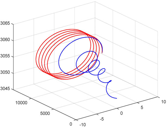
Figure 14.
Missile/target engagement in space (by ZEM).
Proportional navigation is effective, but the reason is not immediately clear. Geometric logic supports issuing acceleration commands based on line-of-sight rates, with a zero rate indicating a collision course. The concept of zero-effort miss helps explain and clarifies this method and aids in developing advanced guidance laws.
5. The Proposed 3D Pure Pursuit Guidance Law
5.1. The Proposed 3D Pure Pursuit Navigation
In this section, we propose an improved version of 3D pure pursuit navigation against a maneuvering target. Unlike traditional 3D pure pursuit, the proposed guidance algorithm adapts the direction but maintains the magnitude of the commanded acceleration proportional to the target acceleration. Let us start by computing the missile acceleration from the classical pure pursuit navigation , which means that
Therefore, the missile acceleration will be
The term . Here, there is some complexity in the formula of because in computing , we need first to evaluate , which is not yet computed; so, in order to overcome such a problem, we assume that the proportional to the target acceleration: , where is a proportionality constant and can be determined by the method proposed by Junaid Farooq in [2].
The validity and performance of the proposed guidance algorithm are investigated through theoretical analysis and numerical simulations. Missiles are controlled by self-contained automatic devices called accelerometers. Accelerometers are inertial devices that measure accelerations. In missile control, they measure the vertical, lateral, and longitudinal accelerations of the controlled missile. But, the problem here is how to calculate the acceleration of the target. Target acceleration in guided missile systems is calculated using a set of integrated techniques and tools that work in parallel to achieve high accuracy in tracking and hitting. These techniques include
- Search and track radar (computational techniques);
- Inertial sensors and Kalman filters;
- Artificial intelligence/machine learning techniques.
In some cases, inertial sensors (such as gyroscopes and accelerometers) mounted on the target itself, if such information is accessible, are used to obtain precise acceleration data. All of these tools and techniques work together to enable the guided missile system to accurately calculate the target’s acceleration, which helps to improve guidance effectiveness and increase the probability of successfully hitting the target.
Engagement Scenarios for 3D PP Navigation (see Algorithm 2): In this simulation (Figure 15), the goal is to assess the performance of various guidance laws under a typical missile–target engagement scenario. The missile is launched with an initial velocity vector aligned toward the target direction from the initial position , aiming to intercept a target initially at , moving with velocity . The target’s acceleration profile is , where and are selected to simulate realistic orbital dynamics. The simulation models the missile’s ability to intercept the target while ensuring computational efficiency. It uses realistic initial conditions for positions and velocities, assuming a perfect seeker that operates under ideal conditions, with no sensor noise and an unrestricted field of view, ensuring an emphasis on guidance system performance rather than hardware limitations. A time step of ensures high-resolution simulation, with control gain selected for realistic performance. The simulation is run in MATLAB R2023 on an processor, offering sufficient computational power for real-time missile dynamic processing.
| Algorithm 2: The Proposed 3D Pure Pursuit Navigation |
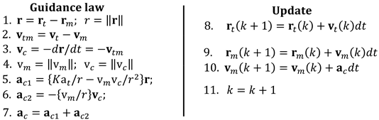 |
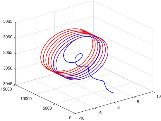
Figure 15.
Missile/target engagement in space (by 3D-PP).
The proposed guidance law’s strength lies in using the target’s speed and acceleration, improving the hit accuracy. Integrating previous methods of data collection, it ensures that the proposed method will pursuit perfectly the target and is also applicable to drones and UAVs. As we can observe, the path is somewhat smooth, without any jerks, unlike the previous example.
5.2. Pure Pursuit Sliding Mode Guidance
As a sliding mode strategy, let us select the manifold as a sliding surface, and then the derivative of this surface concerning time is , but the pure pursuit guidance impose therefore,
The convergence is guaranteed if the states of the dynamic system approach the sliding surface. In order to obtain this condition, we defined the following positive definite function as a Lyapunov function candidate for which its time derivative is . By the Lyapunov theorem, a system is said to be stable if so . If we choose the sliding surface such that with positive definite matrix , then the derivative of is means that which is always satisfied. Next, we aim to select the input acceleration in such a way as to drive to the desired form . To achieve this, we decompose the acceleration into three terms: , where is selected to cancel and the term is selected to nullify the cross product so that we have , and the last term is selected as . Collecting the above accelerations, we obtain
To enhance the convergence of the proposed method, we put
The controller parameters can be determined by the method proposed by Nguyen Xuan-Mung in [54]. Now, let us summarize the proposed algorithm in Algorithm 3.
| Algorithm 3: The Proposed 3D Pure Pursuit Sliding Guidance |
Engagement Scenarios for the PP Sliding Mode (see Algorithm 3): Now, we repeat the same experiment as before, but this time with some realistic sensor noise added to the seeker’s data (e.g., in the form of Brownian noise or Poisson noise). This allows us to assess the method’s robustness against disturbances and evaluate the efficiency of the proposed algorithm.
The results (Figure 16) demonstrate that the guidance algorithm effectively minimizes the miss distance, reducing it from 0.457 m to 0.0132 m, ensuring high accuracy in intercepting the target. The time of closest approach is very short (7.32 s), showcasing the system’s ability to rapidly compute and execute interception trajectories, which is critical in dynamic scenarios. The guidance system also exhibits excellent precision, maintaining accurate tracking and interception even with sensor noise, ensuring a reliable target lock-on. Additionally, it achieves near-perfect tracking by aligning the missile’s trajectory with the target’s path, compensating for target maneuvers, and maintaining course throughout the engagement. This performance reflects advanced control strategies capable of quickly adapting to real-world conditions, ensuring optimal engagement and robust target interception.
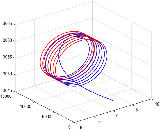
Figure 16.
Missile/target engagement in space (by the proposed 3D-PP sliding mode).
6. Full Simulation Study
6.1. Overall Program Structure
In a digital simulation, processing occurs in discrete time steps, which must be carefully sized to accurately capture the highest frequency components of the missile system (performed in MATLAB R2023 with a step size and solver). At each step, tasks are executed to calculate changes within that interval. Once all tasks for a time increment are completed, the program moves to the next increment and repeats the process. The following flowchart diagram (as illustrated in Figure 17) illustrates this task-to-task processing flow.

Figure 17.
Top-level flow diagram of a flight simulation.
Each block in the diagram represents a major function, group of functions, or a major logic process in the computer program (see Figure 17). The direction of the processing flow is indicated by arrows. One cycle through the flow diagram represents an incremental time step. Missile and target position and velocity vectors and are used to calculate the relative position and velocity vectors with respect to the target. A test is performed to determine whether the missile has reached its closest approach to the target, which of course will not occur until the end of the engagement. If the test shows that the closest approach has been reached, the program sequence is diverted to a routine that calculates miss distance and the program ends. Otherwise, the program continues into the guidance routine.
6.2. The Overall Pseudocode
The presented pseudocode (see Algorithm 4) provides a clear representation of the algorithmic approach employed in this research.
6.3. Optimization Using the PSO Algorithm
Optimization methods are extensively used across various fields to select the best or a satisfactory solution from feasible options. Mathematically, an optimization problem can be expressed as minimizing an objective function , where is an -dimensional vector of decision variables. Swarm intelligence (SI) algorithms simulate systems of individuals using decentralized control and self-organization, inspired by natural groups like ant colonies and bird flocks. These algorithms focus on collective behaviors arising from local interactions. Particle Swarm Optimization (PSO) is an SI algorithm developed by Kennedy and Eberhart in 1995 that is a population-based optimization technique where each particle is defined by its position, velocity, and personal best position , and it identifies the global best particle among all individuals.
- The velocity vector denotes the increment of the current position. It is given for each agent or (particle) by
- = the current velocity of agent at the iteration;
- = inertia weight, takes a value between 0 and 1;
- = inertia weight factor (learning parameters);
- = random vectors, entries take a value of [0, 1];
- = the current position of agent at the kth iteration;
- = the ith agent’s best position;
- = the group’s best position.
- Inertia weight (Function) is given as follows:The inertia can be taken as a constant, typically . This is equivalent to introducing a virtual mass to stabilize the motion of particles, and thus the algorithm is expected to converge more quickly.
- The position vector is modified according to the equationwhere and are the agent’s current and modified positions, and = the agent’s modified velocity [43,50].
Particles should be uniformly distributed initially to sample various regions, which is crucial for multimodal problems. Initial velocities can be set to zero (i.e., ).
6.4. Example of a Simulation
A simulation relies on mathematical models of the missile, target, and environment using equations that describe physical laws and logical sequences. The missile model includes mass, thrust, aerodynamics, guidance, and control, along with equations for calculating its attitude and flight path. The target model, though less detailed, provides data to determine its flight path. The environmental model incorporates atmospheric characteristics and gravity. For illustration, a specific missile configuration with torque-balanced canard control surfaces and cruciform-arranged canards and tail fins is studied. The missile’s description for the simulation model is as follows: is the missile mass at launch, . is the missile mass at burnout, . is the moment of inertia about all axes at launch, , and is the moment of inertia about all axes at burnout, .
is the distance “from the nose to the center of the missile” at the launch moment. is the distance “from the nose to the center of the missile” at the burnout moment. is the distance “from the nose to the ref-station”.
- is the aerodynamic ref length (Missile’s diameter).
- is the fuselage length (from the tile of the missile to the center of mass).
- is the time of burnout.
- is the ref-ambient pressure.
- is the specific impulse and is the lapse rate.
- is the exit area of rocket nozzle.
- is the sound speed in elastic medium.
- is the gas constant.
- is the missile aerodynamic ref area.
- is the air density at sea level.
- is the temperature at sea level.
The aerodynamic forces and moments are computed based on a predefined set of coefficients (see Table 1) that vary as functions of the Mach number.

Table 1.
(Lookup table) Aerodynamic coefficients as functions of .
The thrust force is calculated based on a predefined dataset (see Table 2), where the thrust varies as a function of time.
Table 2.
The ref-thrust produced by a missile motor.
To obtain , we use a numerical interpolation of . The initial missile speed is assumed to apply the instant the missile leaves the launcher. The direction of missile velocity will be calculated in the fire-control routine. (All are in the Earth coordinates)
- is the
- .
- ,
- ,
The initial missile inertial velocity vector expressed in Earth coordinates is transformed into body coordinates using the Earth-to-body reference frame transformation matrix given in subroutine
transformation from Earth to body frame, are components of in the body frame, . inertial velocity vector in the Earth frame,
At the start of the simulation , we put , , and . The initial Euler angles are based on the initial missile centerline vector , and .
- Seeker: time constants , and ,
- Autopilot:
- , ,
- , and
- and
In this study, the missile guidance and control simulation has been conducted to include real-world environmental factors such as sensor noise and wind disturbances. These factors are modeled using turbulence models for wind, with wind gusts having peak speeds up to and turbulence scales of , and more realistic sensor noise models (e.g., ). The target’s path is adjusted by adding random deviations of of the target’s velocity to simulate real-world uncertainties such as wind effects and sensor errors, improving the robustness of the guidance system. Additionally, the simulation has been adapted to account for real-world hardware constraints. The missile’s guidance system has been optimized for embedded systems, taking into consideration size, weight, and power () limitations. Computational loads are reduced by optimizing the guidance algorithm to run efficiently on high-performance CPUs (e.g., ) and GPUs (e.g., ) to handle real-time missile–target engagement with minimal latency. The system is also designed to integrate seamlessly with Hardware-in-the-Loop () simulations, ensuring real-time validation on actual hardware. These improvements make the missile guidance and control system more realistic, operationally feasible, and ready for deployment in real-world scenarios.
For this example of the simulation, it is assumed that the missile altitude at the launch position is at sea level; therefore, a missile altitude above sea level, for use in the atmosphere tables, is given by which is the 3rd component of in the Earth frame. The target is flying at an altitude of and a speed of , and the target flight path is curved and offset laterally from the missile launch site. At the instant of missile launch, the target is inbound at a downrange distance of from the launch site. The time of simulation is limited at , because we need at most to destroy the target.
- The Optimal Proportional Navigation by ZEM:
Figure 18 (left-hand side) shows the missile/target trajectories during the flight, and their interception in 3D. As we see in this figure, the launcher is aimed directly at the target at the time of launch, and the ZEM-PN guidance causes the missile to turn in a direction to lead the target, as is required to strike a moving target. This missile maneuver is initiated when guidance is turned on (0.5 s). At this early time in the flight, the missile speed is slow, which causes the amount of lead, and, therefore, the amount of the maneuver to be overestimated. As the missile gains speed, the missile flight path is corrected until intercept with the target at t = 7.4275 s with a miss-dist = 0.1612 m, as we see in the simulation result. The commanded acceleration (as illustrated in right-hand of Figure 18) is acceptable and starts at a reasonable values and stays close to such demand; this reflects the less energy requirement for the missile guidance. Figure 19 (left-hand side) illustrates the lift and drag variations in ZEM-PN-guided missile engagement. Initially, sharp lift oscillations indicate aggressive maneuvers for trajectory correction, stabilizing as the missile locks onto the target. Drag increases mid-flight due to a high maneuvering effort before decreasing in the terminal phase, reflecting optimized energy management. The results confirm ZEM-PN’s effectiveness in balancing control and aerodynamics for precise interception. Figure 19 (right-hand side) shows the variation in control-surface deflection during flight. Guidance begins after a short “time to go on ”, allowing the missile to gain sufficient speed for control. Afterward, the autopilot commands maneuvers based on the seeker head’s angular rate, with the control system adjusting the surfaces accordingly. Initially, the fins deflect sharply as the seeker locks onto the line of sight and then stabilize for smoother adjustments.
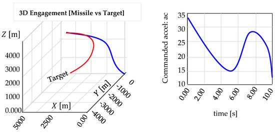
Figure 18.
Missile-Target trajectories and the commanded for optimal ZEM-PN.

Figure 19.
Lift and drag forces with the command inputs for optimal ZEM-PN.
- B.
- The Proposed Optimal 3D Pure Pursuit Guidance:
From the flight path figure (as illustrated in the left-hand side of Figure 20), we can see that the line of sight is tangential to the missile’s path at each instant during the flight until the interception point (or at closet approach), where the miss distance = 0.1497 m at a time t = 7.5070 s. This is the geometry of pure pursuit guidance where the missile’s velocity is always pointing toward the target. In the right-hand side of Figure 20, we notice that the commanded acceleration at the beginning of the pursuit has an acceptable value of 25 ; then, at the end, it increases to a very large value of 150 . This is a worrying matter because it requires very large energy and the missile body may not be able to handle these requirements. To solve this problem, we will see the response of the improved algorithm.
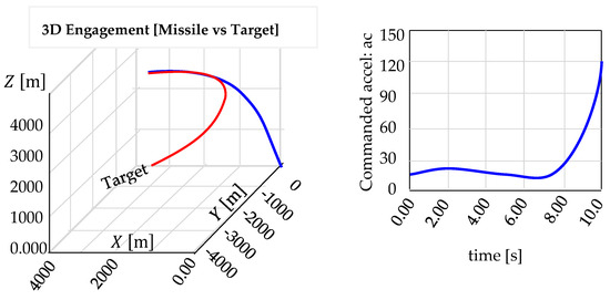
Figure 20.
Missile/Target Trajectories and the commanded for optimal 3D-PP.
The results in Figure 21 highlight the missile’s aerodynamic and control behaviors under the 3D pure pursuit (3D-PP) guidance law. The lift force exhibits oscillations, indicating frequent trajectory adjustments, while drag increases steadily, reflecting a sustained maneuvering effort. Toward the final phase, lift peaks as the missile executes terminal corrections for interception. Command inputs show rapid initial variations, stabilizing mid-flight before increasing again near impact, demonstrating the adaptive nature of 3D-PP in maintaining target pursuit. These results confirm the effectiveness of 3D-PP in achieving dynamic tracking and control while managing aerodynamic forces efficiently.
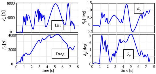
Figure 21.
Lift and drag forces with the command inputs for optimal 3D PP.
- C.
- The Proposed Optimal 3D Sliding Pure Pursuit:
Through the above simulation figures, we have illustrated the effect of the proposed command on the evolution of the flight path during the time of simulation. This method is easily implemented and the optimal desired tracking performance can be obtained by suitably selecting the controller gains using the PSO algorithm.
The use of the or functions instead of in the lateral acceleration equation served to minimize oscillations, reducing chattering and improving system stability and performance in sliding mode control systems. The first figure (left-hand side of Figure 22) shows the two paths of the missile and target, and their interception point at time with a miss distance = 0.1598 m. From the right-hand side of Figure 22, we can also observe that the required acceleration is not excessively high. It starts relatively elevated and then decreases toward the end of the pursuit, stabilizing at a value of . This indicates that the controller does not require a significant amount of energy. On the other hand, we notice that the noise does not affect the control at all.

Figure 22.
M/T trajectories with the commanded for 3D Sliding PP.
Comparison of the Above Simulation Results: Now, let us perform the comparison between the three results in terms of the time of the closest approach and the miss distance.
The proposed 3D-pure pursuit sliding command shows good tracking (even in a noisy environment), and records the lowest miss distance in the shortest time; thus, it is the most robust guidance law. The command to line of sight has also good results for the miss distance, even if it took more time than the other two methods. The 3D-PP command marked acceptable results due to the utilization of optimized gains (it is effective in its control strategy but consumes more energy compared to other methods). Table 3 also shows that the ZEM scored the lowest miss distance, while the 3D-PP sliding guidance scored the shortest time of closest approach.
Table 3.
Comparison of the simulation results.
6.5. Simulation of Interception Under Varying Conditions
In order to understand all the aspects and circumstances surrounding the proposed method (sliding pure pursuit), we conducted several simulations, as shown in Figure 23 (the most left and the middle ones), where we launched the missile toward a moving, maneuvering target in a spiral motion (the middle Figure 23); from different initial positions toward a maneuvering target in a curved motion with some disturbances (right-hand side of Figure 23); and launched it from the same place, under the same conditions, and with different guidance laws (the most left side of Figure 23). Each time, we recorded the basic parameters (as illustrated in Table 4 and Table 5) of the shortest approach time, the maximum speed upon collision, the maximum acceleration, the path angle, the impact angle, the load factor, and other parameters in order to discover the strength and effectiveness of the proposed control.
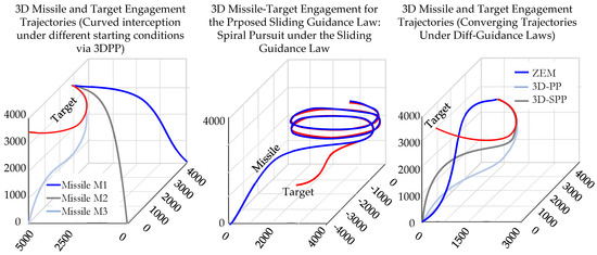
Figure 23.
3D engagement trajectories of M-T under various guidance laws and initial conditions.
Table 4.
The test of different guidance laws with a curved path and the same initial conditions.
Table 5.
The test of different starting points with the same guidance law (3D-SPP guidance).
The tests in Figure 23 demonstrate that 3D-SPP guidance consistently outperforms the other methods. It achieves a relatively small miss distance, the fastest time to closest approach, and the highest approach speed, ensuring quick and precise interception. While the spiral trajectory in Figure 23 is smoother, it results in slower engagement and less optimal acceleration. In contrast, sliding pursuit shows superior maneuverability, lower energy dissipation, and a more efficient flight path, ensuring better targeting and impact angles for a lethal strike. In light of the following considerations,
- A lower ensures precise interception.
- A shorter leads to rapid convergence.
- A higher supports successful interception but requires efficient control.
- A higher acceleration provides maneuverability but adds structural stress.
- The load factor measures the missile’s ability to withstand G-forces.
- The flight path and impact angles affect trajectory efficiency and lethality.
- Control effort impacts actuator demand and precision.
From these factors, we deduce that 3D sliding pursuit guidance outperforms other methods by achieving small miss distances, fast convergence, and high maneuverability. It optimizes energy usage and ensures effective engagement angles, making it the most efficient guidance law for precise, rapid, and lethal interception.
To implement the proposed 3D sliding pursuit guidance in real-world missile systems, the hardware must be carefully selected and optimized to meet stringent computational performance, SWaP constraints, and sensor integration requirements. The system should rely on high-performance embedded processors (e.g., multi-core CPUs, GPUs, and FPGAs), efficient low-power electronics, and robust sensor and actuator systems. By optimizing these hardware aspects, the proposed guidance law can be effectively deployed in operational missile systems, ensuring rapid, precise, and reliable target interception.
7. Conclusions
The proposed 3D SPP guidance demonstrated significant improvements over conventional methods, showing faster interception times and higher precision in tracking moving targets. Compared with established algorithms like ZEM and 3D-PP, it achieved the shortest time to closest approach and the lowest miss distance. The algorithm’s robustness to noise and efficient energy usage were key highlights, confirming its effectiveness for real-world applications. Additionally, it outperformed other methods in dynamic tracking and handling uncertainties such as wind disturbances. The use of an optimized control strategy based on PSO further enhanced its performance, making it both efficient and suitable for real-world applications. This work gives a foundation for future research in guidance systems and control, promising enhanced accuracy and reliability. Future work can extend this approach to multi-agent systems, enhancing guidance in more complex operational scenarios.
Author Contributions
B.B., conceptualization, data curation, formal analysis, investigation, methodology, project administration, resources, software, visualization, writing—original draft. G.F.F., conceptualization, funding acquisition, investigation, supervision, resources, writing—original draft. M.R., project administration, validation, writing—review and editing. K.H., data curation, methodology, validation, writing—review and editing. All authors have read and agreed to the published version of the manuscript.
Funding
This research received no external funding.
Institutional Review Board Statement
Not applicable.
Informed Consent Statement
Not applicable.
Data Availability Statement
All data supporting the findings are included within the article.
Conflicts of Interest
The authors declare that they have no known competing financial interests or personal relationships that could have appeared to influence the work reported in this paper.
Abbreviations
The following abbreviations are used in this manuscript:
| ZEM | Zero-Effort Miss Distance |
| PP | Pure Pursuit |
| PN | Proportional Navigation |
| LOS | Line of Sight |
| CLOS | Command to Line of Sight |
| 3D | Three-Dimensional |
| SAM | Surface-to-Air Missiles |
| PNG | Proportional Navigation Guidance |
| BTT | Bank-to-Turn |
| LQG | Linear Quadratic Gaussian |
| RF | Radio Frequency |
| RTD | Radians To Degrees |
| PSO | Particle Swarm Optimization |
| SI | Swarm Intelligence |
Appendix A
Planer Motion (Rigid Bodies): Let be a vector position of a body located at time , at point . The polar coordinates of the body are , where and . From Euler identity, we have ; so, . The complex exponential represents a radial vector of a unit length in the Cartesian plan. The velocity and acceleration vectors can be written in polar forms
with
Keeping in mind that is a unit radial vector, we can understand why is called a unit transverse vector— rotates counterclockwise by . Notice that , , and . The Cartesian and polar forms are as follows:
Relative Planer Motion: When the body moves in a fixed frame , then the polar frame will be in motion with respect to the fixed one. If we define the rotational vector of the body to be with , then
The index stands for the Cartesian frame. From the fact
we obtain
And, by using , , , and ,
Notice that
Then, we obtain
Now, let us interpret the acceleration in relative frames
Using the facts that , , and
we obtain
Now, assume that the missile position is denoted by and the target position is ; then, we have , which means that
Using the fact , we obtain
Finally, we obtain the fundamental diff-equation of the navigation problem
Now, let us compute the acceleration of the missile
Relative Motion in 3D Space: In such a case, you have
References
- Paul, Z. Tactical and Strategic Missile Guidance. In Progress in Astronautics and Aeronautics AIAA, 4th ed.; American Institute of Aeronautics & Astronautics Inc.: Reston, VR, USA, 2019. [Google Scholar] [CrossRef]
- Farooq, J. Hybrid Deep Neural Network for Data-Driven Missile Guidance with Maneuvering Target. Def. Sci. J. 2023, 73, 602–611. [Google Scholar] [CrossRef]
- He, S. Three-Dimensional Optimal Impact Time Guidance for Antiship Missiles. J. Guid. Control Dyn. 2019, 42, 941–948. [Google Scholar] [CrossRef]
- Wang, C.; Yan, J.; Lyu, R.; Liang, Z.; Chen, Y. Optimal Guidance Law for Critical Safe Miss Distance Evasion. Aerospace 2024, 11, 1041. [Google Scholar] [CrossRef]
- Jeon, I.S. Optimality of P-Navigation based on Nonlinear Formulation. IEEE Trans. Aerosp. Electron. Syst. 2010, 46, 2051–2055. [Google Scholar] [CrossRef]
- Cho, N.; Kim, Y. Optimality of Augmented Ideal Proportional Navigation for Maneuvering Target Interception. IEEE Trans. Aerosp. Electron. Syst. 2016, 52, 948–954. [Google Scholar] [CrossRef]
- Kim, H.-G. Integrated Autopilot Guidance Based on Zero-Effort-Miss Formulation for Tail-Controlled Missiles. Appl. Sci. 2022, 12, 7120. [Google Scholar] [CrossRef]
- Gutman, S. 3D-Nonlinear Vector Guidance and Exo-Atmospheric Interception. IEEE Trans. Aerosp. Electron. Syst. 2015, 51, 4. [Google Scholar] [CrossRef]
- Zhang, G. Structure Synchronized Dynamic Event-Triggered Control for Marine Ranching AMVs via the Multi-Task Switching Guidance. IEEE Trans. Intell. Transp. Syst. 2024, 25, 20295–20308. [Google Scholar] [CrossRef]
- Li, J. Integrating Dynamic Event-Triggered and Sensor-Tolerant Control: Application to USV-UAVs Cooperative Formation System for Maritime Parallel Search. IEEE Trans Intell. Transp. Syst. 2024, 25, 3986–3998. [Google Scholar] [CrossRef]
- Wang, W.; Wu, M.; Chen, Z.; Liu, X. Integrated Guidance-and-Control Design for Three-Dimensional Interception Based on Deep-Reinforcement Learning. Aerospace 2023, 10, 167. [Google Scholar] [CrossRef]
- Yan, T.; Liu, C.; Gao, M.; Jiang, Z.; Li, T. A Deep Reinforcement Learning-Based Intelligent Maneuvering Strategy for the High-Speed UAV Pursuit-Evasion Game. Drones 2024, 8, 309. [Google Scholar] [CrossRef]
- Choi, W.-J.; Lee, J.-S. A Balanced Path-Following Approach to Course Change and Original Course Convergence for Autonomous Vessels. J. Mar. Sci. Eng. 2024, 12, 1831. [Google Scholar] [CrossRef]
- Zhao, J. Cooperative guidance of seeker-less missile considering localization error. Chin. J. Aeronaut. 2019, 32, 1933–1945. [Google Scholar] [CrossRef]
- Chen, C.-H. Design of Midcourse Guidance Laws via a Combination of Fuzzy and SMC Approaches. Int. J. Control Autom. Syst. 2010, 8, 272–278. [Google Scholar] [CrossRef]
- Liu, X. Target Tracking Enhancement by Three-Dimensional Cooperative Guidance Law Imposing Relative Interception Geometry. Aerospace 2021, 8, 6. [Google Scholar] [CrossRef]
- Tahk, M.J.; Shim, S.W.; Hong, S.M.; Choi, H.L.; Lee, C.H. Impact Time Control Based on Time-to-Go Prediction for Sea-Skimming Antiship Missiles. IEEE Trans. Aerosp. Electron. Syst. 2018, 54, 2043–2052. [Google Scholar] [CrossRef]
- Hodžić, M. Missile Guidance using Proportional Navigation and Machine Learning. J. Eng. Res. Sci. 2024, 3, 19–26. [Google Scholar] [CrossRef]
- Scott, B. Guidance of a homing missile via nonlinear geometric control methods. J. Guid. Control Dyn. 1995, 18, 441–448. [Google Scholar]
- Rusnak, I. Optimal Guidance for High-Order and Acceleration Constrained Missile. J. Guid. Control Dyn. 1991, 14, 383–391. [Google Scholar] [CrossRef]
- Liang, H. Optimal Guidance Laws for a Hypersonic Multiplayer Pursuit-Evasion Game Based on a Differential Game Strategy. Aerospace 2022, 9, 97. [Google Scholar] [CrossRef]
- Yang, C.D. Analytical Solution of Three-Dimensional Realistic True Proportional Navigation. J. Guid. Control Dyn. 1996, 19, 7504–7509. [Google Scholar] [CrossRef]
- Li, Z. Field-to-View Constrained Integrated Guidance and Control for Hypersonic Homing Missiles Intercepting Supersonic Maneuvering Targets. Aerospace 2022, 9, 640. [Google Scholar] [CrossRef]
- Alibani, M. A Fuzzy Guidance System for Rendezvous and Pursuit of Moving Targets. Robotics 2020, 9, 110. [Google Scholar] [CrossRef]
- Shinar, J. Robust pursuit of a hybrid evader. Appl. Math. Comput. 2010, 217, 1231–1245. [Google Scholar] [CrossRef]
- Shinar, J. Three Dimensional Optimal Pursuit and Evasion with Bounded Control. IEEE Trans. Autom. Control 1980, 25, 492–496. [Google Scholar] [CrossRef]
- Shinar, J. Solution Techniques for Realistic Pursuit-Evasion Games. In Advances in Control and Dynamic Systems; Leondes, C.T., Ed.; Academic Press: Amsterdam, The Netherlands, 1981; Volume 17. [Google Scholar]
- Berglund, E. Guidance and Control Technology, Defense Technical Information Center Compilation Part Notice ADP010953; Defense Technical Information Center: Fort Belvoir, VA, USA, 2001. [Google Scholar]
- Oleg, M.; Zhang, K. Pursuit Problem of Unmanned Aerial Vehicles. Mathematics 2023, 11, 4162. [Google Scholar] [CrossRef]
- Sui, Y. A Fuzzy Pure Pursuit for Autonomous UGVs Based on Model Predictive Control and Whole-Body Motion Control. Drones 2024, 8, 554. [Google Scholar] [CrossRef]
- Su, Z. Evade Unknown Pursuer via Pursuit Strategy Identification and Model Reference Policy Adaptation (MRPA) Algorithm. Drones 2024, 8, 655. [Google Scholar] [CrossRef]
- Li, Z. Research on Head Pursuit Interception Strategy for Hypersonic Target. Appl. Sci. 2023, 13, 4772. [Google Scholar] [CrossRef]
- Shima, T. Optimal Cooperative Pursuit and Evasion Strategies Against a Homing Missile. J. Guid. Control. Dyn. 2011, 34, 414–425. [Google Scholar] [CrossRef]
- Shima, T. Head Pursuit Guidance. J. Guid. Control. Dyn. 2007, 30, 1437–1444. [Google Scholar] [CrossRef]
- Yamasaki, T. Sliding mode-based pure pursuit guidance for unmanned aerial vehicle rendezvous and chase with a cooperative aircraft. Proc. IMechE Part G J. Aerosp. Eng. 2010, 224, 1057–1067. [Google Scholar] [CrossRef]
- Kumar, S.R. Finite-Time Impact Time Guidance using Deviated Pursuit against Maneuvering Targets. In Proceedings of the American Control Conference Denver, Denver, CO, USA, 1–3 July 2020. [Google Scholar]
- Don, L. Hommertzheim. Training an artificial neural network the pure pursuit maneuver. Comput. Oper. Res. 1991, 18, 343–353. [Google Scholar]
- Jerger, J.J. Systems Preliminary Design; U.S. Naval Air Development Center, Inc.: Patuxent River, MD, USA, 1960. [Google Scholar]
- U.S. Army Missile Command. Military Handbook: Missile Flight Simulation, Part One Surface-To-Air Missiles; MIL-HDBK-1211(MI); U.S. Government Printing Office: Washington, DC, USA, 1995.
- Siouris, G.M. Missile Guidance and Control Systems; Springer: New York, NY, USA, 2004. [Google Scholar]
- Hawley, P.A.; Blauwkamp, R.A. Six-Degree-of-Freedom Digital Simulations for Missile Guidance, Navigation, and Control. Johns Hopkins APL Tech. Dig. 2010, 29, 71–84. [Google Scholar]
- Özkan, B. Modeling of dynamics, guidance, and control systems of air-to-surface missiles. J. Def. Model. Simul. Appl. Methodol. Technol. 2012, 9, 101–112. [Google Scholar] [CrossRef]
- Belkacem, B. Advanced Strategies for Guidance & Control of SAM Missiles; Lambert Academic Publishing: Chisinau, Moldova, 2024. [Google Scholar]
- Yanushevsky, R. Modern Missile Guidance; Kiev Polytechnic Institute: Kyiv, Ukraine; Taylor, Francis: Abingdon, UK, 2019. [Google Scholar]
- Arthur, S.L. Principles of Guided Missile Design; Naval Air Development Center: Warminster Township, PA, USA; D. Van Nostrand Company, Inc.: New York, NY, USA, 1955. [Google Scholar]
- Mohan, R.S. Fundamentals of Guided Missiles; Defense Research and Development Organization: New Delhi, India, 2016. [Google Scholar]
- Palumbo, N.F. Basic Principles of Homing Guidance. Johns Hopkins APL Tech. Digest 2010, 29, 25–41. [Google Scholar]
- Shneydor, N.A. Missile Guidance and Pursuit: Kinematics, Dynamics and Control; Israel Institute of Technology: Chichester, UK, 1998. [Google Scholar]
- Jackson, P.B. Overview of Missile Flight Control Systems. Johns Hopkins APL Tech. Digest 2010, 29, 9–24. [Google Scholar]
- Chen, Y.-W. Dynamic interception point guidance algorithm based on particle swarm optimization. Meas. Control 2022, 55, 983–995. [Google Scholar] [CrossRef]
- Yamasaki, T. Modified Command to Line-of-Sight Intercept Guidance for Aircraft Defense. J. Guid. Control. Dyn. 2013, 36, 898–902. [Google Scholar] [CrossRef]
- Ahi, B. Novel command to line of sight guidance with practical limitations. Asian J. Control 2021, 24, 1426–1436. [Google Scholar] [CrossRef]
- Turetsky, V. Minimum Effort Pursuit Guidance with Delayed Engagement Decision. J. Guid. Control Dyn. 2019, 42, 1310–1319. [Google Scholar] [CrossRef]
- Xuan-Mung, N.; Nguyen, N.P.; Pham, D.B.; Dao, N.N.; Nguyen, H.T.; Ha Le Nhu Ngoc, T.; Vu, M.T.; Hong, S.K. Novel gain-tuning for sliding mode control of second-order mechanical systems: Theory and experiments. Sci. Rep. 2023, 13, 10541. [Google Scholar] [CrossRef] [PubMed]
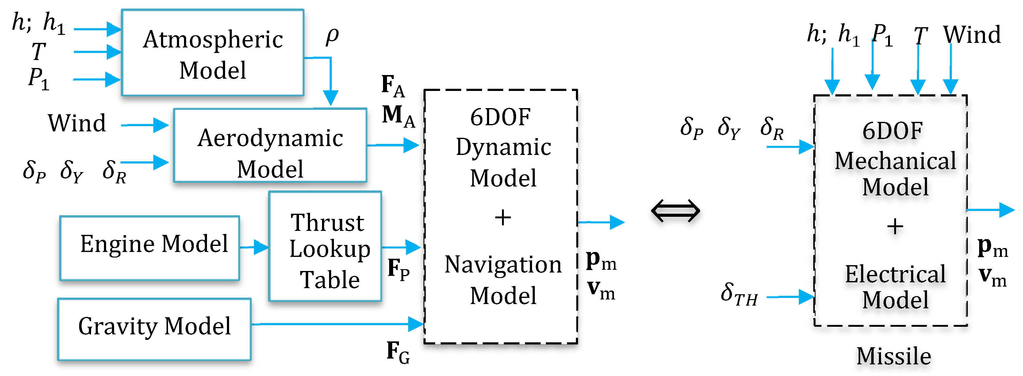
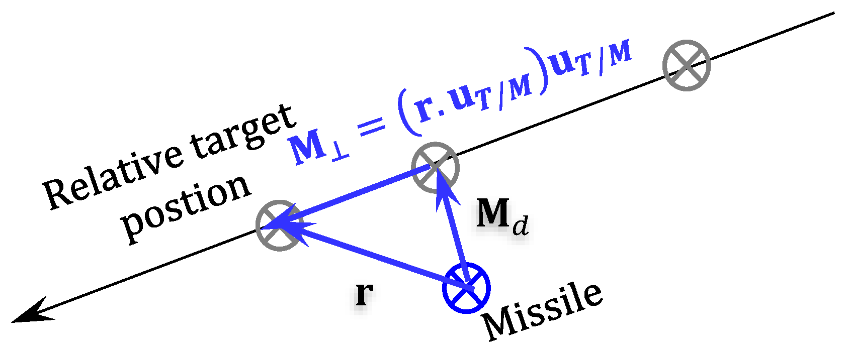

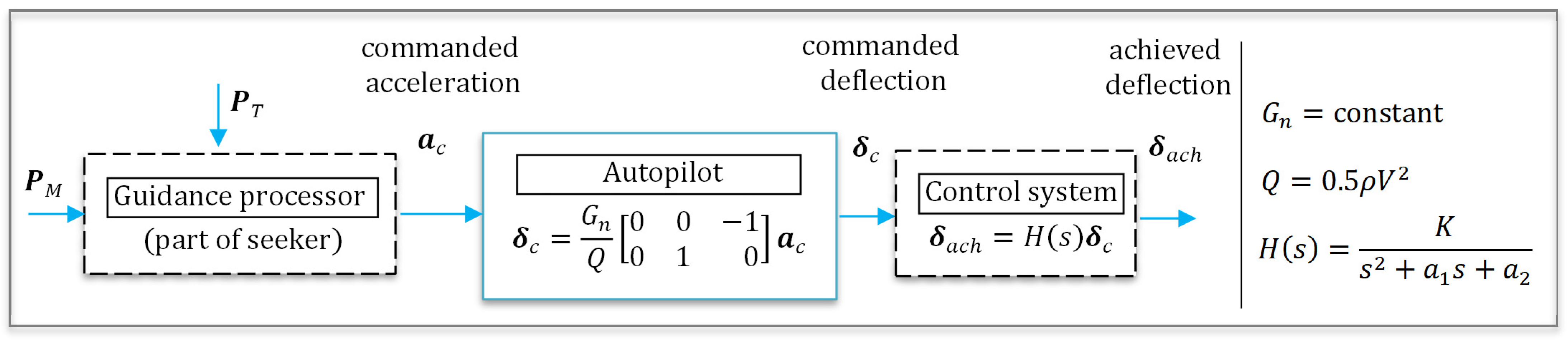
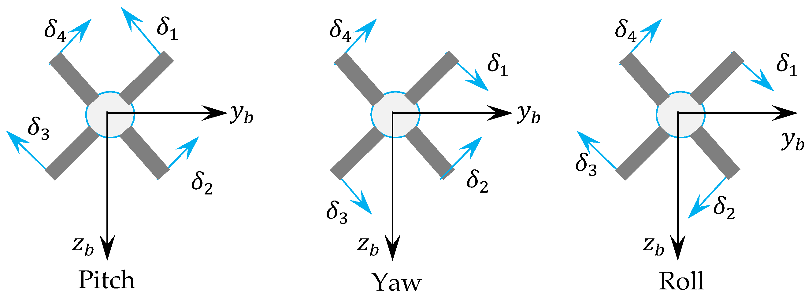
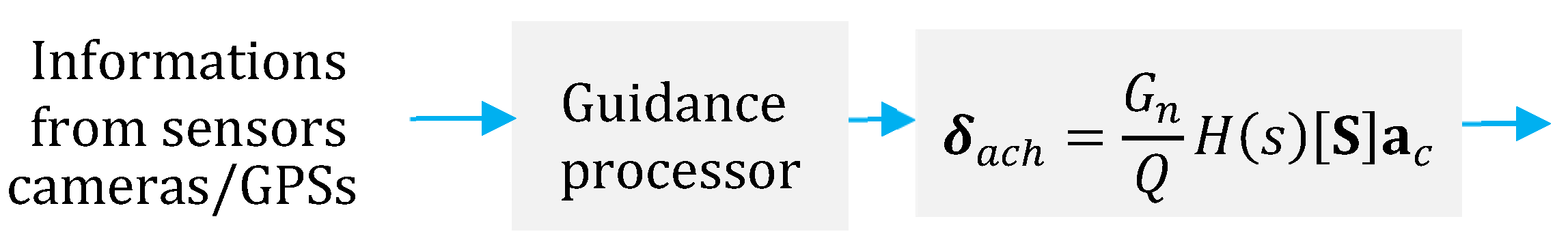

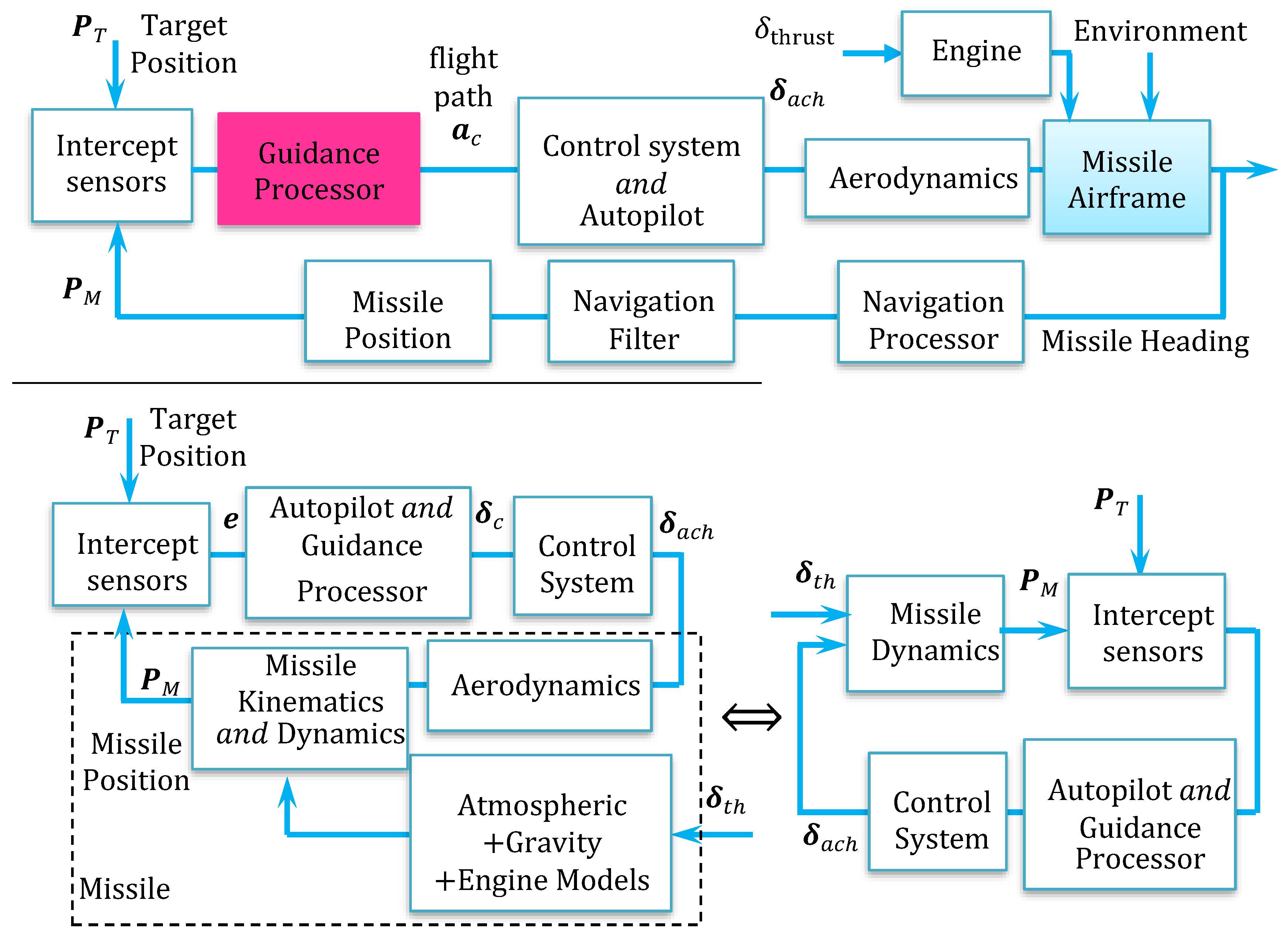
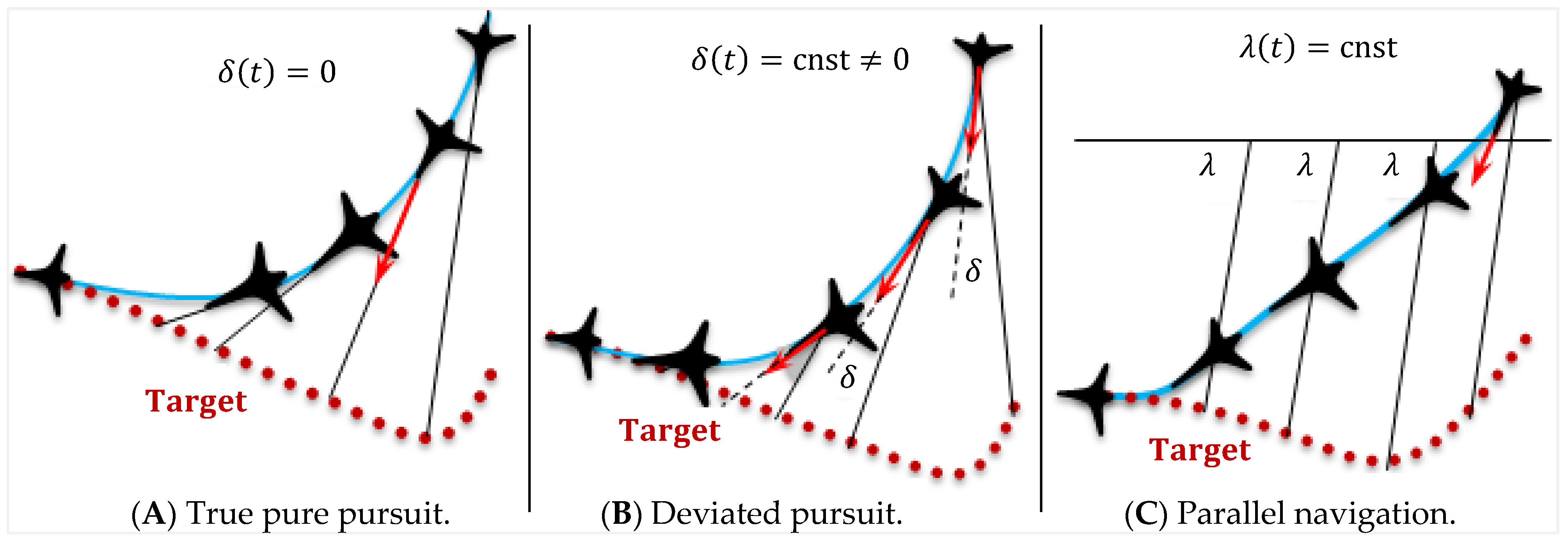

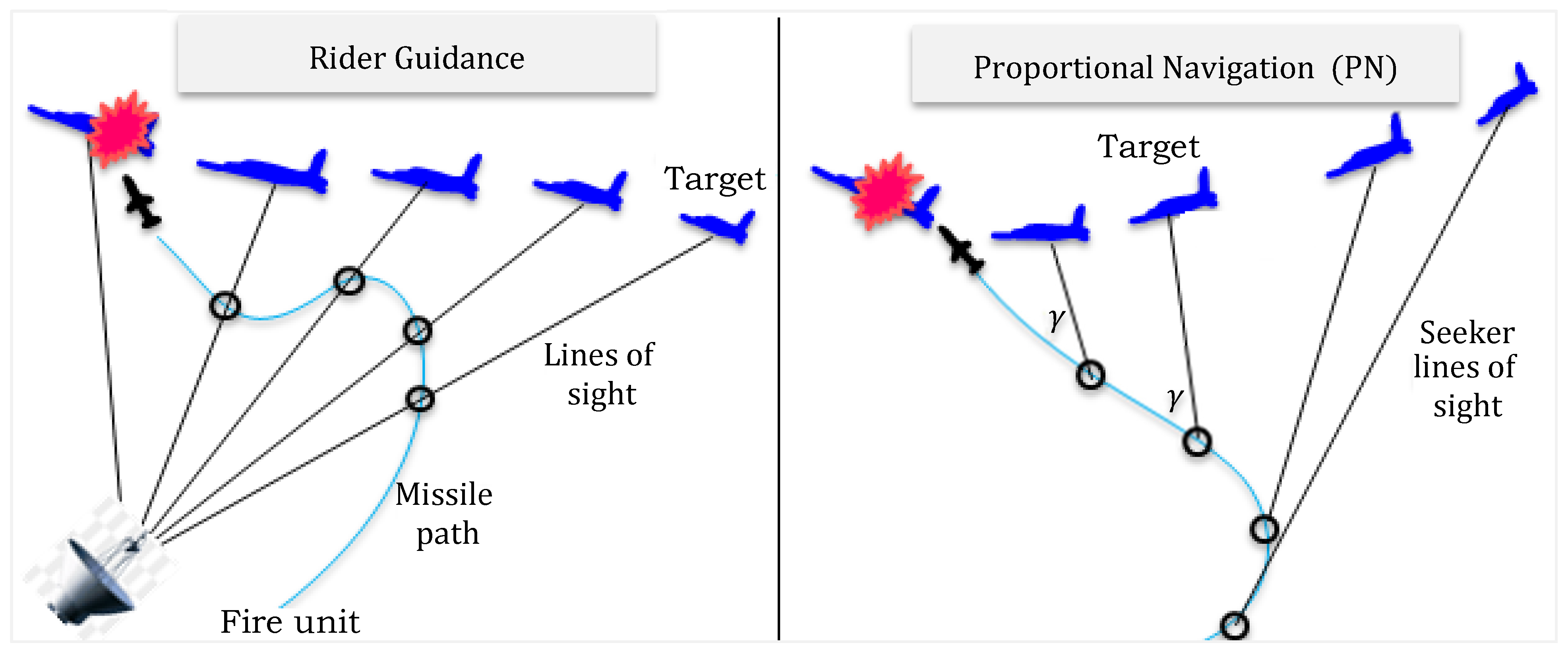
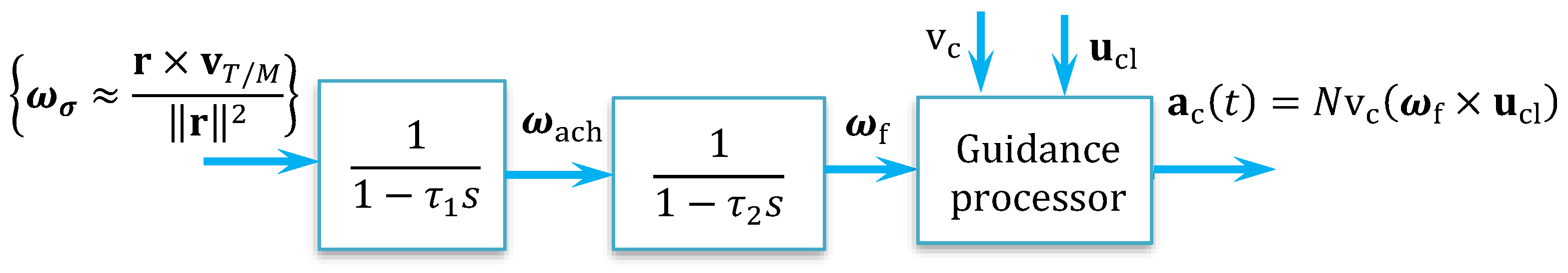

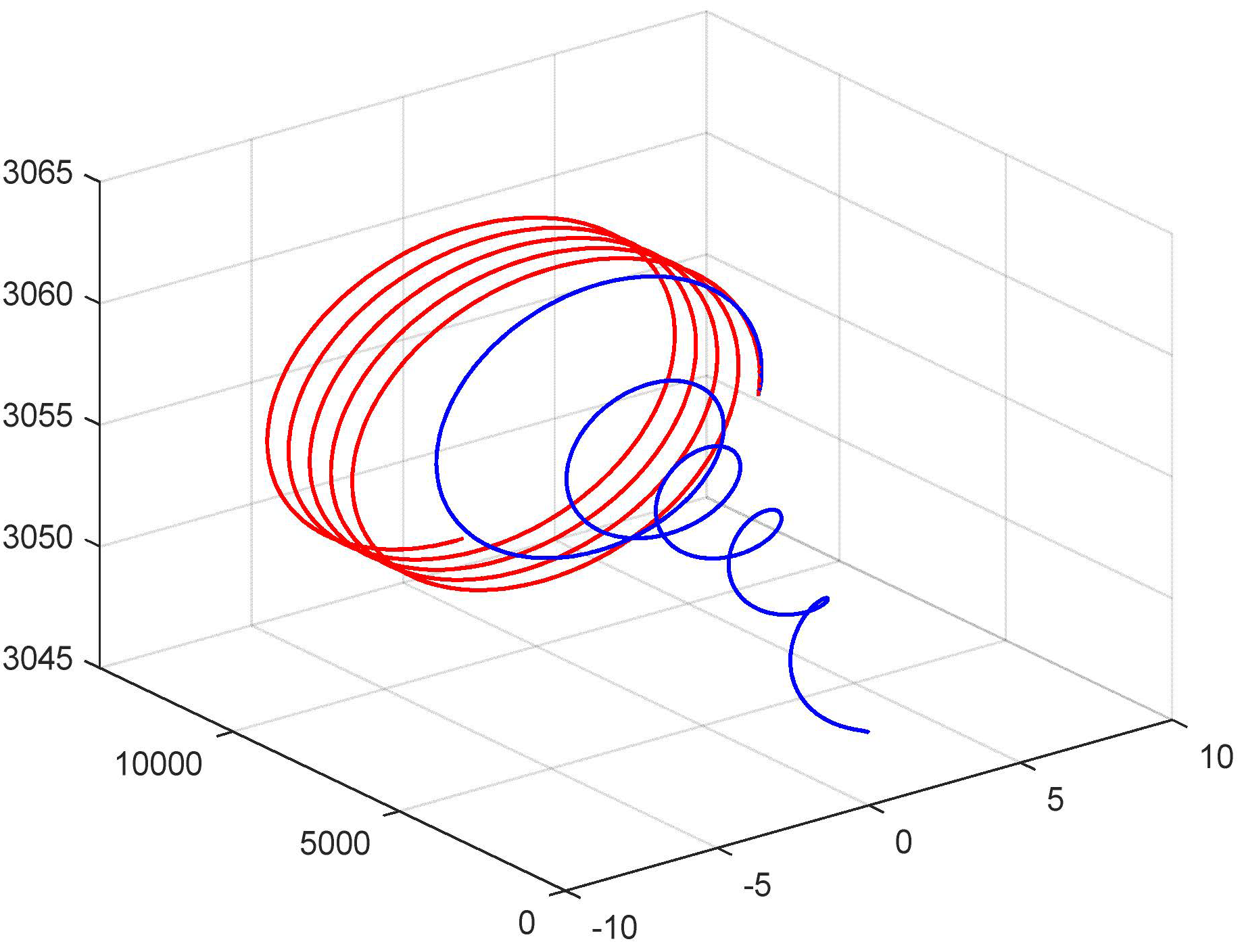
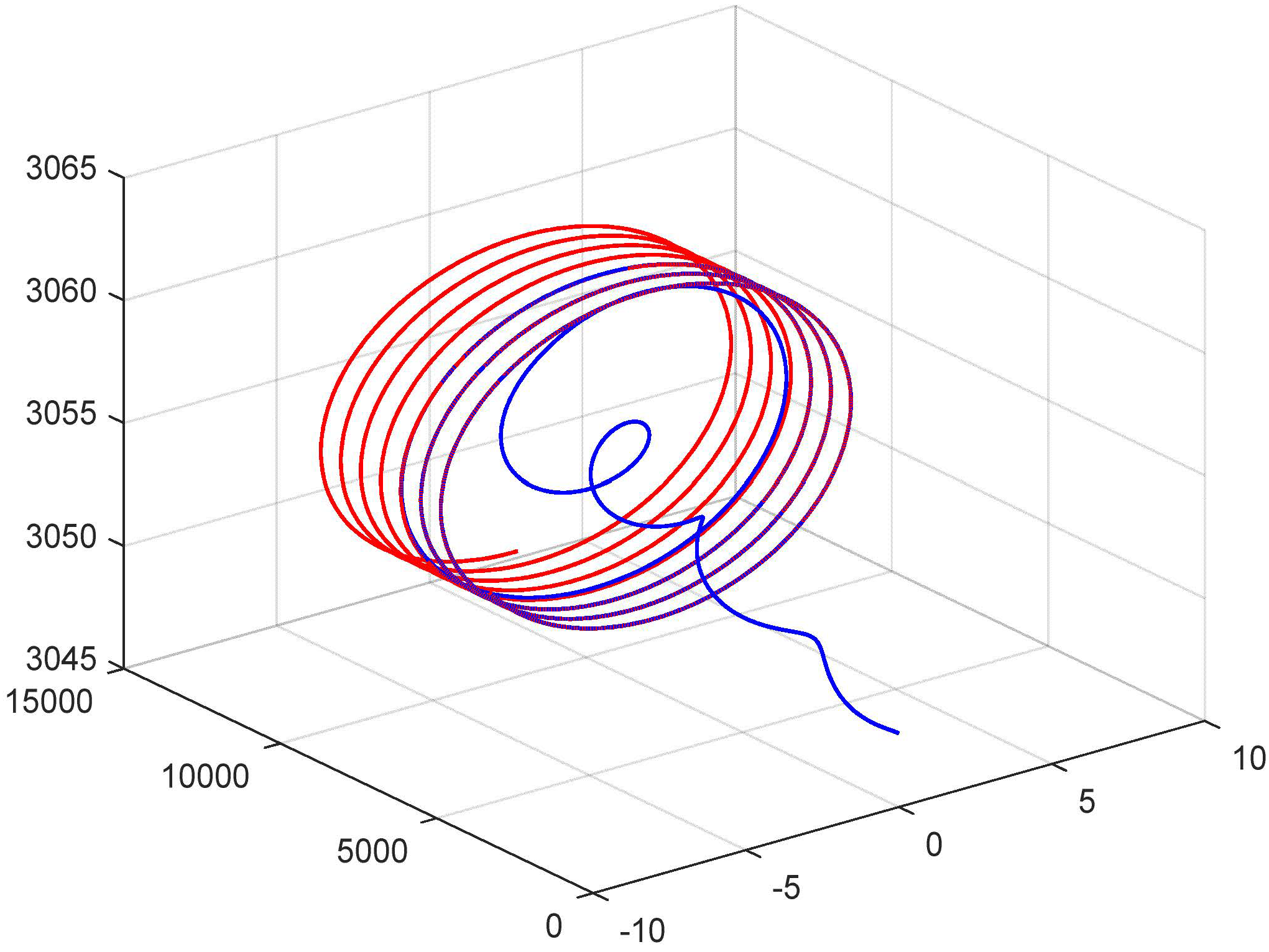
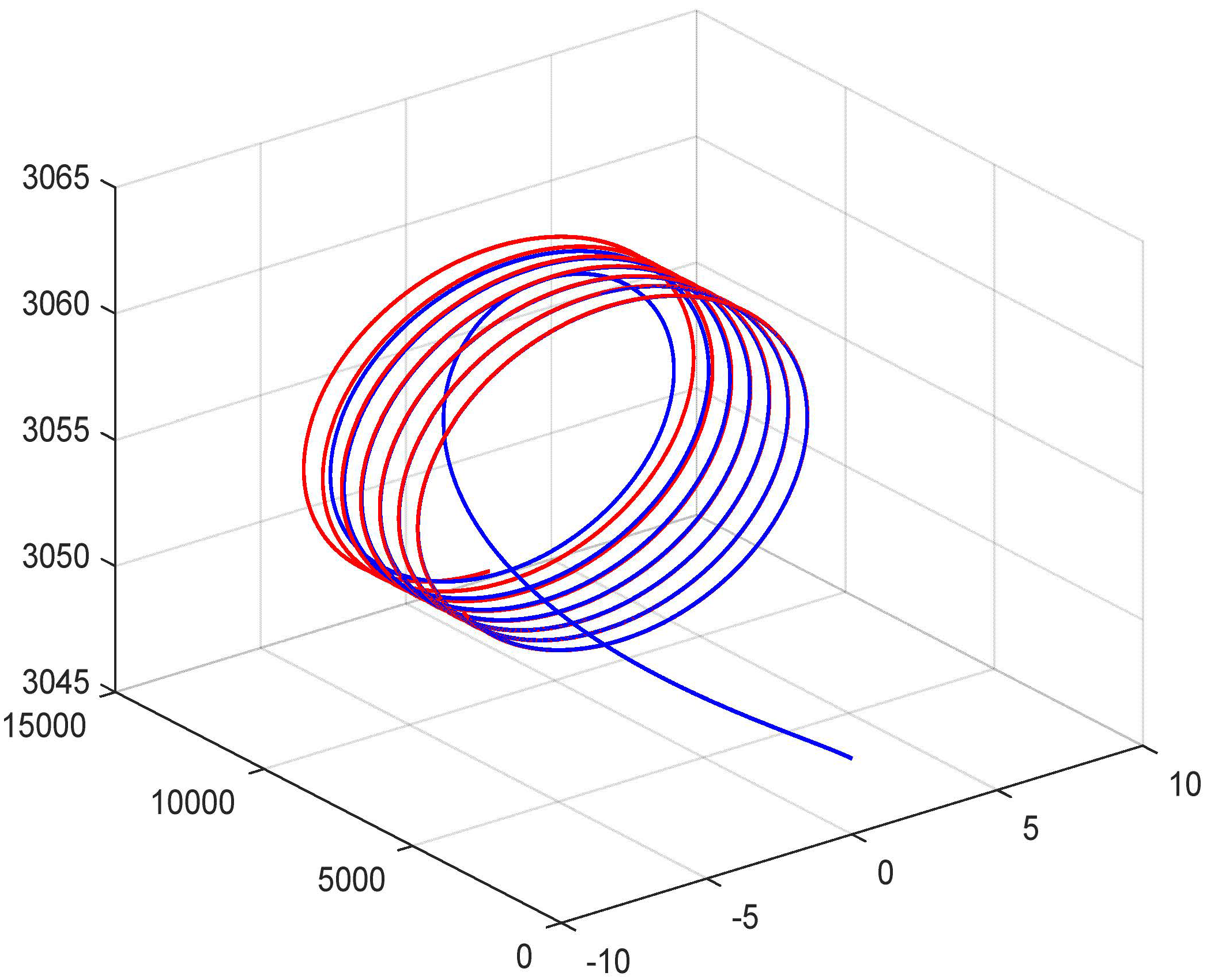
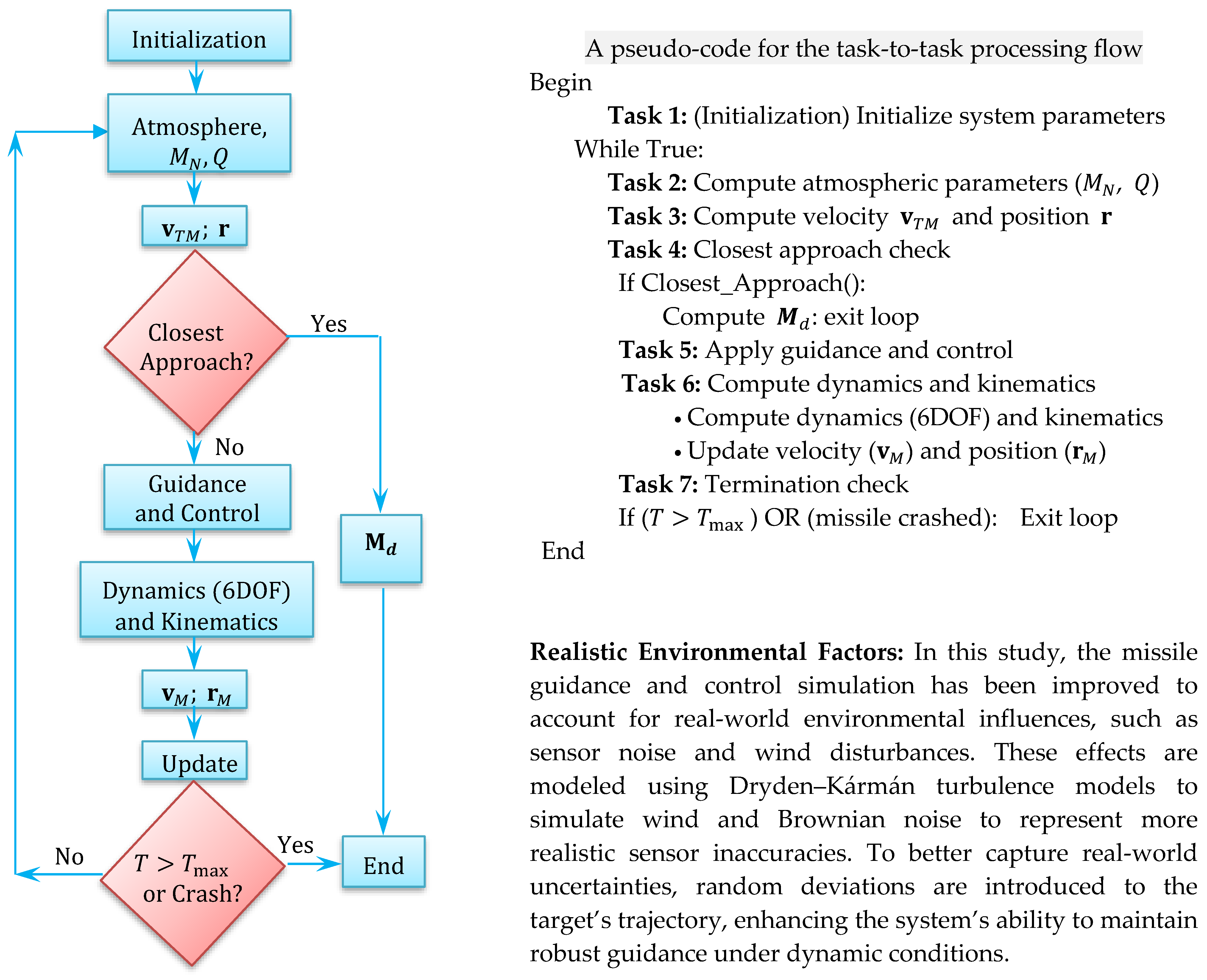
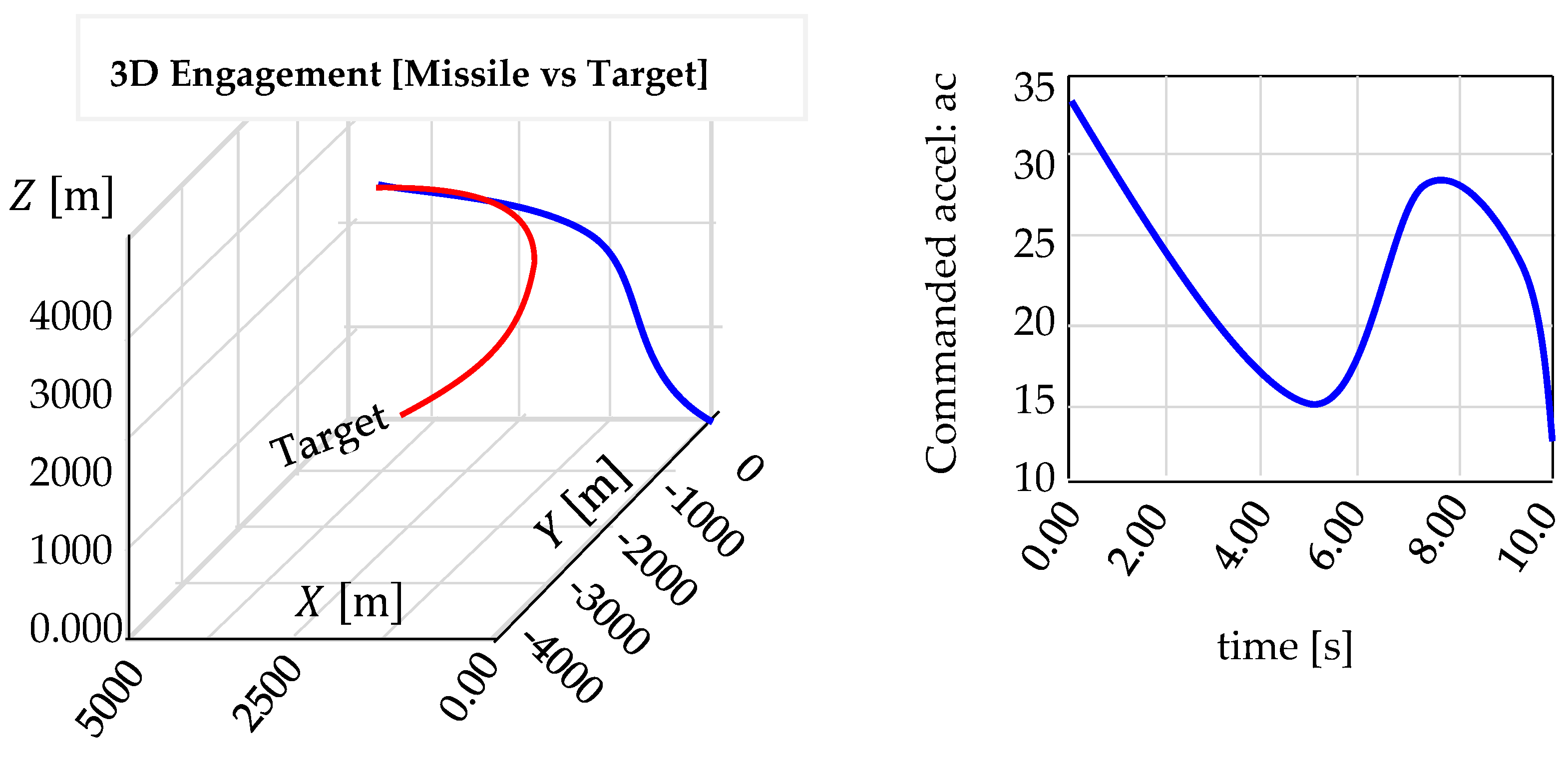
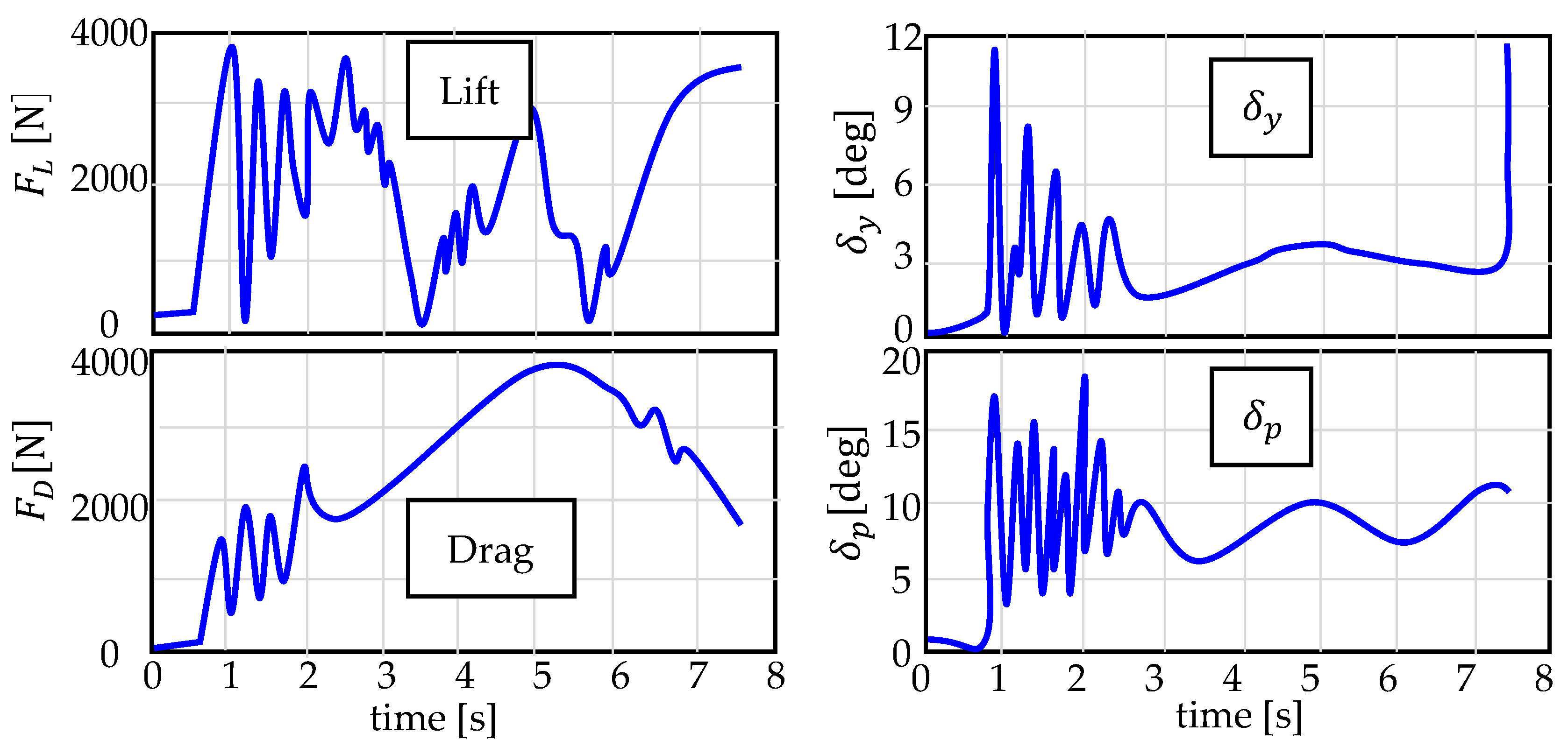
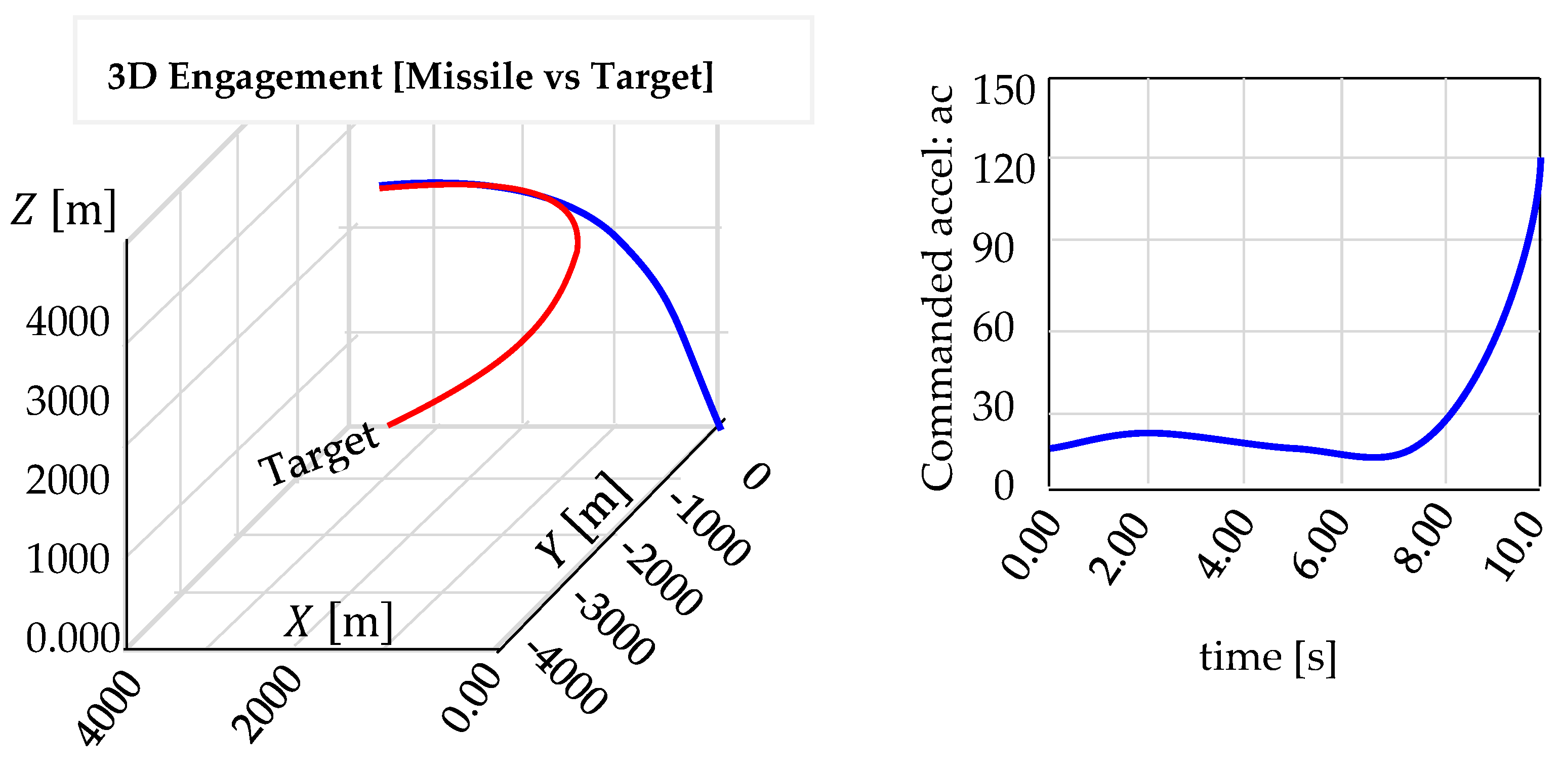
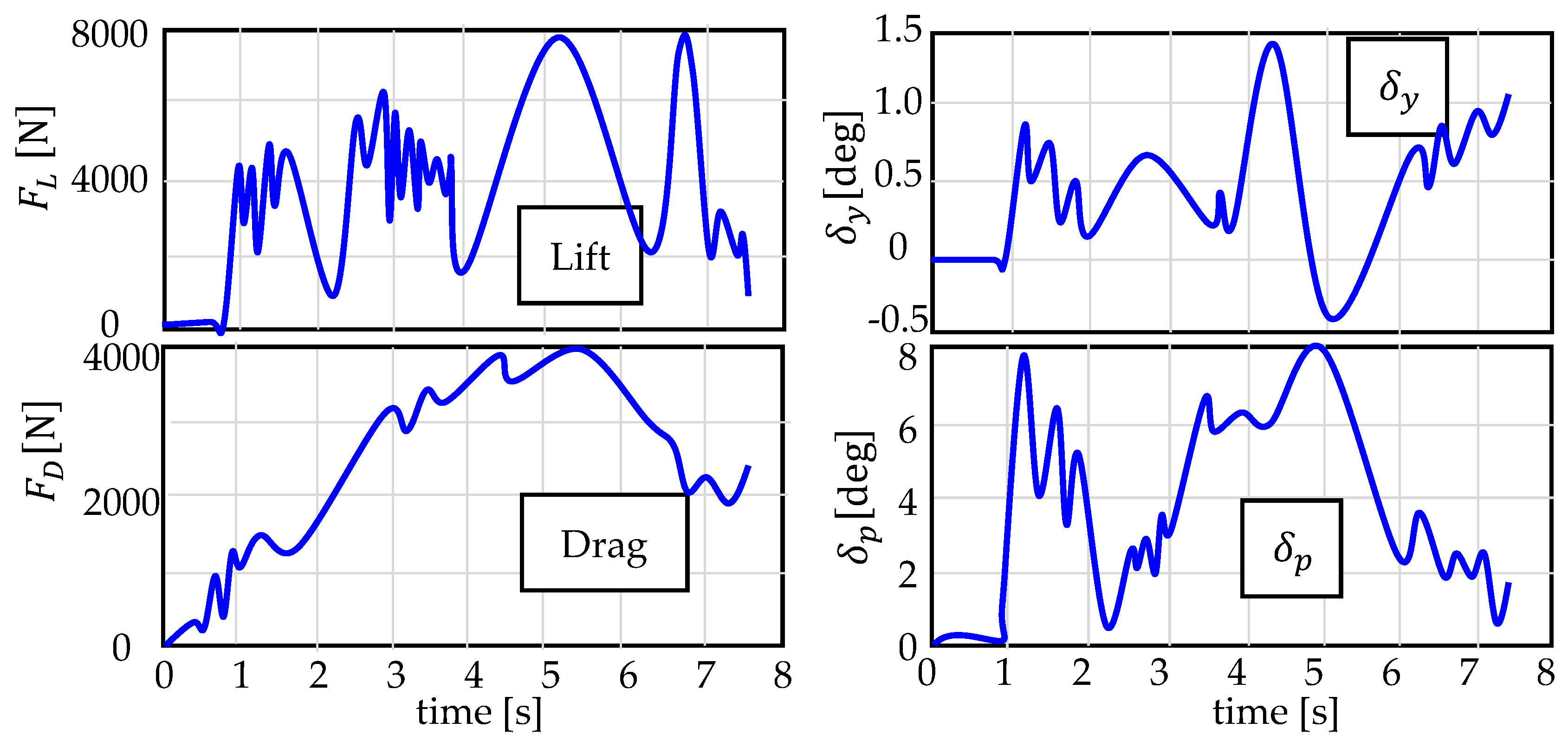
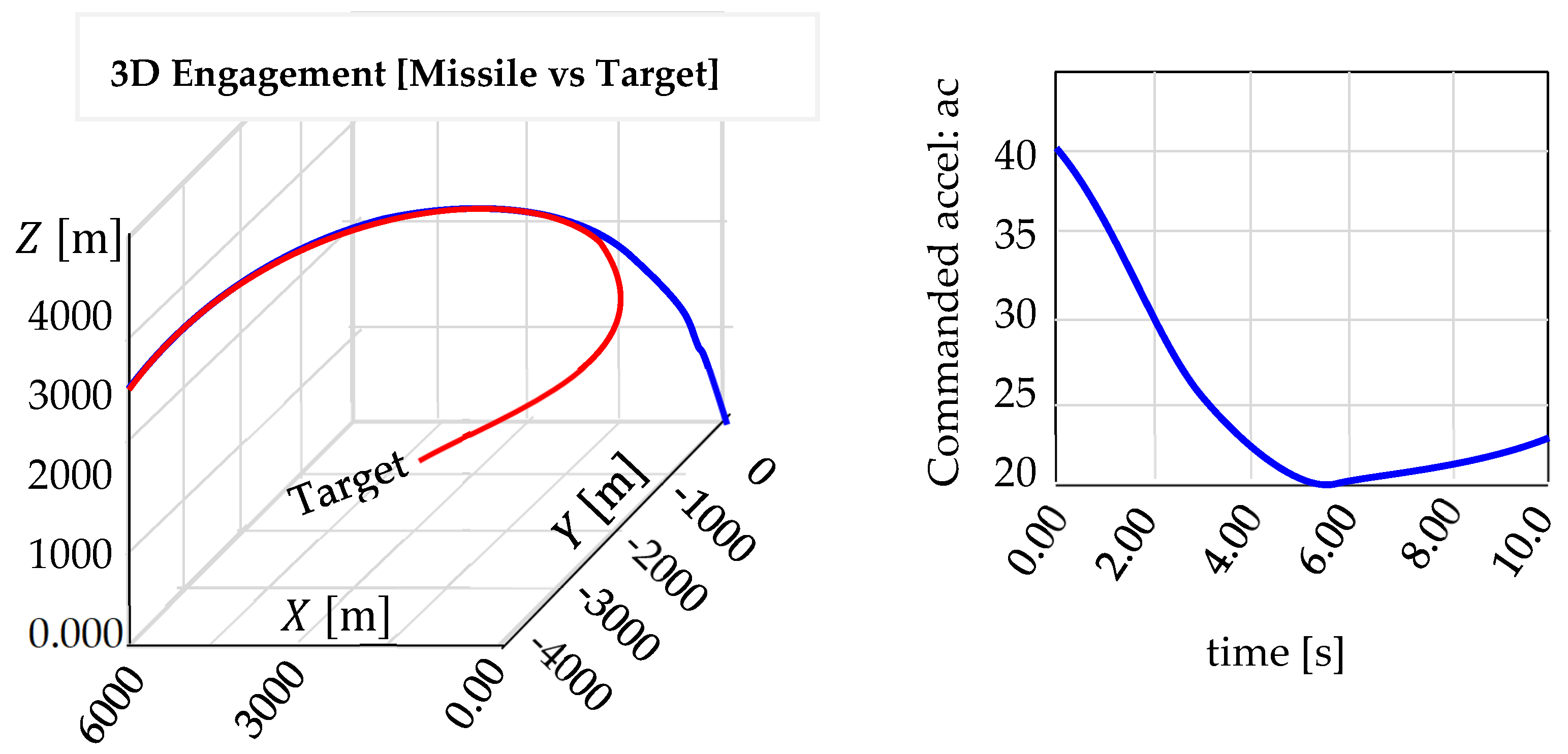
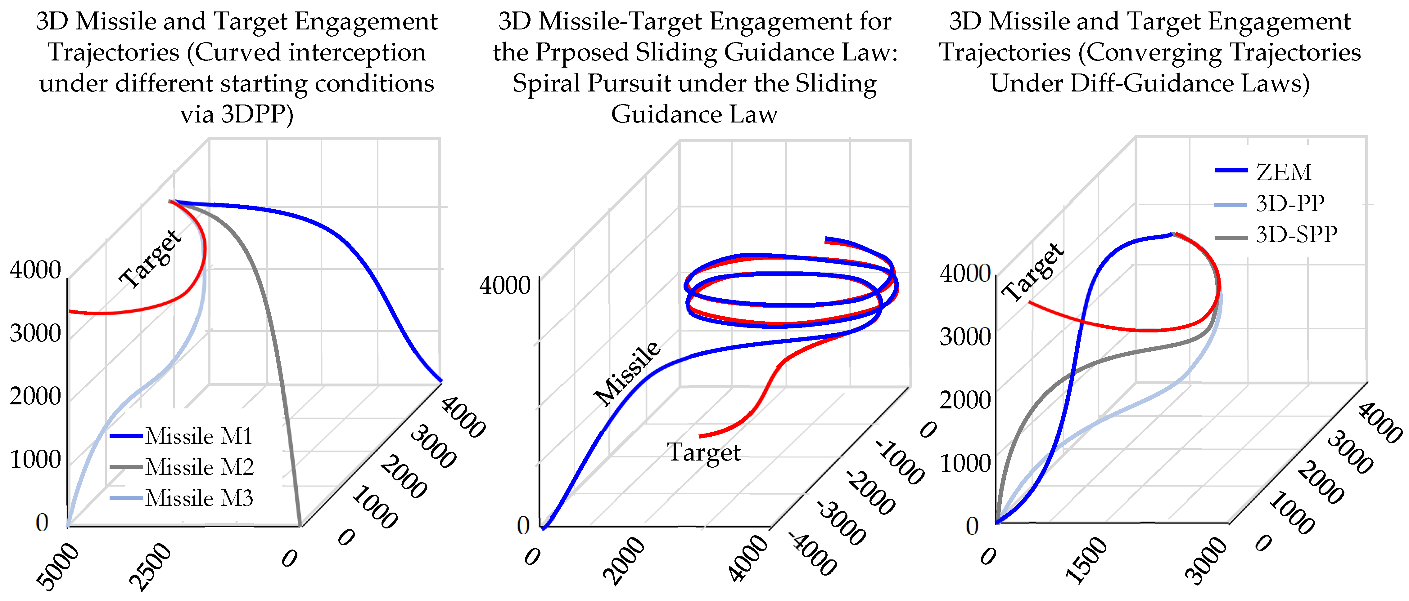
Disclaimer/Publisher’s Note: The statements, opinions and data contained in all publications are solely those of the individual author(s) and contributor(s) and not of MDPI and/or the editor(s). MDPI and/or the editor(s) disclaim responsibility for any injury to people or property resulting from any ideas, methods, instructions or products referred to in the content. |
© 2025 by the authors. Licensee MDPI, Basel, Switzerland. This article is an open access article distributed under the terms and conditions of the Creative Commons Attribution (CC BY) license (https://creativecommons.org/licenses/by/4.0/).