Abstract
Image compression is a critical area of research aimed at optimizing data storage and transmission while maintaining image quality. This paper explores the application of clustering techniques as a means to achieve efficient and high-quality image compression. We systematically analyze nine clustering methods: K-Means, BIRCH, Divisive Clustering, DBSCAN, OPTICS, Mean Shift, GMM, BGMM, and CLIQUE. Each technique is evaluated across a variety of parameters, including block size, number of clusters, and other method-specific attributes, to assess their impact on compression ratio and structural similarity index. The experimental results reveal significant differences in performance among the techniques. K-Means, Divisive Clustering, and CLIQUE emerge as reliable methods, balancing high compression ratios and excellent image quality. In contrast, techniques like Mean Shift, DBSCAN, and OPTICS demonstrate limitations, particularly in compression efficiency. Experimental validation using benchmark images from the CID22 dataset confirms the robustness and applicability of the proposed methods in diverse scenarios.
Keywords:
image compression; clustering techniques; K-Means; BIRCH; divisive clustering; DBSCAN; OPTICS; mean shift; GMM; BGMM; CLIQUE 1. Introduction
Image compression is a critical field in computer science and digital communication, playing a vital role in reducing the storage and transmission requirements of digital images without significantly compromising their quality [1]. With the proliferation of multimedia applications, the demand for efficient compression techniques has increased exponentially. From social media platforms and cloud storage services to real-time video streaming [2] and medical imaging systems [3], the ability to store and transmit high-resolution images efficiently is paramount. Traditional compression methods have served well over the years; however, as technology evolves, so does the need for innovative techniques that address modern challenges, such as scalability, adaptability to different image types, and the ability to preserve essential details in various contexts [4].
Clustering techniques have emerged as a promising solution in the realm of image compression [5]. These methods leverage the inherent structure and patterns within an image to group similar pixel blocks into clusters. Each cluster is represented by a centroid, significantly reducing the amount of data needed to reconstruct the image [6]. Unlike traditional approaches that rely on predefined transformations or quantization schemes, clustering-based methods are data-driven and adaptive, making them well-suited for diverse image types and resolutions [7]. By analyzing and exploiting the spatial and spectral redundancies within images, clustering techniques can achieve high compression ratios while maintaining acceptable visual fidelity [8].
This paper explores the application of nine clustering techniques to image compression: K-Means, Balanced Iterative Reducing and Clustering using Hierarchies (BIRCH), Divisive Clustering, Density-Based Spatial Clustering of Applications with Noise (DBSCAN), Ordering Points to Identify the Clustering Structure (OPTICS), Mean Shift, Gaussian Mixture Model (GMM), Bayesian Gaussian Mixture Model (BGMM), and Clustering In Quest (CLIQUE). Each method offers unique advantages and challenges, depending on the characteristics of the image and the specific parameters used. One of the critical research questions is the importance of parameter tuning in achieving optimal results. For example, the choice of block size significantly impacts the performance of each technique [9]. Smaller block sizes often yield higher SSIM values (structural similarity index), preserving fine details in the image, but they also result in lower compression ratios due to the increased granularity [10]. Conversely, larger block sizes improve compression efficiency at the expense of detail retention, leading to pixelation and reduced visual fidelity. Similarly, clustering-specific parameters, such as the grid size in CLIQUE or the epsilon value in DBSCAN, play a pivotal role in determining the quality and efficiency of compression [11]. This underscores the need for a tailored approach when applying clustering techniques to image compression, taking into account the specific requirements of the application [12].
Several studies have demonstrated the effectiveness of K-Means in image compression. For example, Afshan et al. [13] compared K-Means with other clustering-based approaches and found it to be computationally efficient, particularly for images with distinct color regions. Similarly, a study by Baid and Talbar [14] highlighted that K-Means-based image compression significantly reduces file sizes while maintaining good image quality, as measured by metrics like PSNR and SSIM.
Divisive clustering has been explored in image compression research for its ability to adaptively determine cluster structures. Fradkin et al. [15] found that Divisive Clustering outperformed K-Means in preserving fine-grained details in images with complex textures. Additionally, it has been used to improve vector quantization techniques by dynamically determining cluster sizes.
DBSCAN has been applied in image compression, particularly for segmenting images with irregular regions. A study by Jaseela and Ayaj [16] showed that DBSCAN-based compression achieved better edge preservation compared to K-Means, particularly for medical and satellite images. Since DBSCAN identifies noise pixels separately, it is also useful for removing redundant details in noisy images.
GMM-based clustering is widely used in image compression due to its ability to model complex data distributions. According to Fu et al. [17], GMMs outperform K-Means in handling overlapping clusters and representing natural images with smooth transitions. Moreover, GMM-based compression has been successfully used in medical imaging, where subtle variations in intensity need to be preserved.
This paper provides a comprehensive exploration of clustering techniques for image compression, analyzing their performance in balancing image quality and compression efficiency. The major contributions of this paper are as follows:
- It includes an in-depth review of nine clustering techniques: K-Means, BIRCH, Divisive Clustering, DBSCAN, OPTICS, Mean Shift, GMM, BGMM, and CLIQUE.
- A comparative analysis highlights the key characteristics, strengths, and limitations of each technique. This includes insights into parameter sensitivity, handling of clusters with varying densities, overfitting tendencies, computational complexity, and best application scenarios.
- The paper outlines a universal framework for image compression using clustering methods, including preprocessing, compression, and decompression phases.
- Each clustering technique was implemented to achieve image compression by segmenting image blocks into clusters and reconstructing them using cluster centroids.
- The implementations are adapted for diverse clustering methods, ensuring consistency in the preprocessing, compression, and decompression phases.
- The paper provides detailed analysis and interpretation for each clustering technique, addressing trade-offs between compression and quality.
- Rigorous experiments were conducted using benchmark images from CID22 to validate compression efficiency and image quality for all clustering techniques.
- The results are synthesized into a clear discussion, ranking the techniques based on their effectiveness in achieving a balance between CR (compression ratio) and SSIM.
- Custom visualizations demonstrate the impact of varying block sizes and parameters for each technique, offering intuitive insights into their performance characteristics.
The remainder of this paper is organized as follows. Section 2 presents the vector quantization approach and its use in image compression. Section 3 provides a detailed review of various clustering techniques, categorized into partitioning, hierarchical, density-based, distribution-based, and grid-based methods, along with a comparative analysis of their strengths and weaknesses. Section 4 presents the implementation and experimental evaluation of these clustering techniques, focusing on their performance across diverse datasets and configurations. Section 5 explains the compression and decompression processes facilitated by clustering methods, highlighting the role of clustering in achieving efficient image compression. Section 6 discusses the quality assessment metrics used to evaluate compression performance. Section 7 delves into the performance analysis of clustering techniques for image compression, providing insights into their efficiency and effectiveness. Section 8 validates the results using the CID22 dataset, demonstrating the practical applicability of the methods in real-world scenarios. Finally, Section 9 concludes the paper by summarizing the findings and proposing directions for future work.
2. Vector Quantization and Its Use in Image Compression
2.1. Fundamentals of Vector Quantization
VQ is a quantization technique that represents large datasets using a finite set of representative vectors. Unlike scalar quantization, which processes individual pixel values independently, VQ groups multiple pixel values into vectors and maps them to the closest representative vector from a predefined codebook. The primary components of VQ are:
- Codebook: A collection of representative vectors;
- Encoding: The process of mapping input vectors to the closest codebook vector;
- Decoding: The reconstruction of the original data using the codebook indices.
Mathematically, VQ operates by partitioning an N-dimensional vector space into K regions, each associated with a codeword. Given an input vector x, the closest codeword c is selected based on a distance metric, typically the Euclidean distance. The codebook is generated using clustering techniques such as K-Means, which iteratively refine the codewords to minimize the distortion error [18].
2.2. Vector Quantization in Image Compression
Image compression aims to reduce the amount of data required to represent an image while preserving its perceptual quality. VQ plays a crucial role in this process through the following steps:
- Training Phase: The codebook is created by selecting a representative set of image blocks (e.g., 4 × 4 or 8 × 8 pixel blocks) from a collection of training images. These blocks are clustered to form the codebook [19].
- Encoding Phase: Each image block in the input image is mapped to the closest codeword in the codebook, and its index is stored instead of the original block.
- Decoding Phase: The compressed image is reconstructed by replacing each stored index with the corresponding codeword from the codebook.
The key advantage of VQ in image compression is that it significantly reduces the bit rate required for storage and transmission while maintaining a visually acceptable image quality. Moreover, it exploits the spatial redundancy inherent in images by grouping similar patterns together [20].
3. Overview of Clustering Techniques
3.1. Partitioning Techniques
Partitioning clustering techniques divide a dataset into a set number of clusters by optimizing a specific objective function, such as minimizing the distance between data points and their assigned cluster centers [21]. These methods require the user to specify the number of clusters in advance and are generally efficient for large datasets where a clear partitioning structure is desired [22].
3.1.1. K-Means
K-Means clustering is a widely used technique in data analysis that seeks to partition a dataset into a specified number of distinct groups, known as clusters [23]. The process begins by randomly selecting a set of initial centroids, each representing the center of a potential cluster. These centroids serve as starting points for the clustering process [24].
The algorithm then enters an iterative phase where each data point in the dataset is assigned to the nearest centroid, effectively grouping the data points into clusters based on their proximity to these central points [25]. The assignment for the i-th data point to the j-th centroid is given by:
Once all points are assigned, the centroids are recalculated by taking the mean of all data points within each cluster, ensuring that the centroids move to the center of their respective clusters:
where is the set of data points assigned to the j-th cluster and is the number of data points in that cluster.
This process of assignment and centroid recalculation repeats until convergence, which occurs when the centroids no longer shift significantly between iterations [25]. At this stage, the clusters are considered stable, and the algorithm halts. The final output is a partitioning of the dataset into clusters, with each data point assigned to one of the clusters based on its distance to the centroids.
K-Means is particularly effective for datasets with spherical clusters of similar size and density, and it is valued for its simplicity and efficiency [26]. However, it does have limitations, such as sensitivity to the initial placement of centroids and difficulties in handling clusters of varying shapes and densities [27]. Despite these challenges, K-Means remains a foundational tool in the field of cluster analysis, widely used in applications ranging from market segmentation to image compression [28].
3.1.2. BIRCH
Balanced Iterative Reducing and Clustering using Hierarchies, commonly known as BIRCH, is a hierarchical clustering algorithm designed for large datasets [29]. It aims to create compact summaries of data through a multi-phase process that efficiently builds clusters while minimizing memory usage and computational time.
The process begins with the construction of a Clustering Feature (CF) Tree, a height-balanced tree structure that summarizes the dataset [30]. The CF Tree is composed of Clustering Features, which are tuples representing subclusters. Each Clustering Feature stores essential information about a subcluster, including the number of points, the linear sum of points, and the squared sum of points. This compact representation allows BIRCH to handle large datasets efficiently.
As data points are sequentially inserted into the CF Tree, the algorithm identifies the appropriate leaf node for each point [31]. If the insertion of a point causes the diameter of a leaf node to exceed a predefined threshold, the node splits, and the tree adjusts to maintain its balance. This dynamic insertion process ensures that the CF Tree remains balanced and compact.
Once the CF Tree is built, BIRCH proceeds to the clustering phase. It can use various clustering algorithms, such as agglomerative clustering or K-Means, to further refine the clusters [32]. The leaf nodes of the CF Tree, which contain compact summaries of the data, serve as input for this phase. By clustering these summaries instead of the entire dataset, BIRCH significantly reduces the computational complexity.
BIRCH’s strength lies in its ability to handle large datasets with limited memory resources [31]. The CF Tree structure enables incremental and dynamic clustering, making it well-suited for data streams and situations where the entire dataset cannot be loaded into memory simultaneously. The algorithm efficiently adjusts to changes in the dataset, maintaining its performance even as new data points are added.
However, BIRCH has some limitations. The initial phase, which involves building the CF Tree, is sensitive to the choice of the threshold parameter that controls the diameter of the leaf nodes [32]. An inappropriate threshold value can lead to suboptimal clustering results. Additionally, while BIRCH handles large datasets efficiently, it may not perform as well with very high-dimensional data, where the curse of dimensionality affects the clustering quality.
3.2. Hierarchical Techniques
Hierarchical clustering techniques build a tree-like structure of nested clusters by either iteratively merging smaller clusters into larger ones (agglomerative) or splitting larger clusters into smaller ones (divisive) [33]. These methods do not require a predetermined number of clusters and are well-suited for exploring the hierarchical relationships within the data.
Divisive Clustering
Divisive Clustering, also known as top-down hierarchical clustering, is a method that begins with the entire dataset as a single, all-encompassing cluster and progressively splits it into smaller and more refined clusters [34]. This approach is fundamentally different from its counterpart, agglomerative clustering, which starts with individual data points and merges them into larger clusters.
The process is initiated by treating the whole dataset as one large cluster. The algorithm then identifies the most appropriate way to divide this cluster into two smaller clusters :
where and are the centroids of the sub-clusters and , respectively.
This is typically performed by finding the split that maximizes the dissimilarity between the resulting sub-clusters while minimizing the dissimilarity within each sub-cluster [34]. Various techniques, such as K-Means clustering or other splitting criteria, can be employed to determine the optimal division. Once the initial split is made, the algorithm treats each of the resulting clusters as separate entities and recursively applies the same splitting procedure to each cluster. This recursive division continues, creating a hierarchical tree structure, until each cluster contains only a single data point or a predefined number of clusters is reached.
Divisive Clustering excels at identifying global cluster structures because it starts with the entire dataset [35]. This holistic perspective allows it to make large-scale divisions that might be missed by methods that build up clusters from individual points. However, this approach can be computationally intensive, as each split requires considering all possible ways to partition the data.
Despite its computational demands, Divisive Clustering is particularly effective for datasets with a clear hierarchical structure or when the goal is to uncover large, distinct groupings within the data [34]. It is a powerful tool in the data analyst’s arsenal, capable of revealing deep insights into the underlying patterns and relationships within complex datasets.
3.3. Density-Based Techniques
Density-based clustering techniques identify clusters by locating regions in the data space where data points are denser compared to the surrounding areas [36]. These methods do not require a predefined number of clusters, making them particularly effective in discovering clusters of arbitrary shapes and handling noise within the data.
3.3.1. DBSCAN
Density-Based Spatial Clustering of Applications with Noise, commonly known as DBSCAN, is a clustering technique that groups together data points that are closely packed while marking outliers as noise [37]. Unlike traditional clustering methods that focus on distance to centroids, DBSCAN identifies clusters based on the density of data points.
The process begins by defining two key parameters: (epsilon), the maximum distance between two points for one to be considered in the neighborhood of the other, and , the minimum number of points required to form a dense region (a cluster). With these parameters set, the algorithm starts with an arbitrary point in the dataset [38]. If this point has at least points within a radius of , it is marked as a core point, and a new cluster is initiated. The algorithm then iteratively examines all points within the radius of the core point. If these neighboring points meet the criterion, they are added to the cluster, and their neighborhoods are also explored. This process continues until no more points can be added to the cluster.
Points that do not have enough neighbors to form a dense region but are within distance of a core point are labeled as border points and are included in the nearest cluster. Points that do not fall within the radius of any core point are considered noise and are left unclustered.
DBSCAN excels at identifying clusters of arbitrary shapes and sizes, making it particularly effective for datasets with irregular or non-spherical clusters [39]. Moreover, it automatically determines the number of clusters based on the data’s density structure, eliminating the need for a pre-specified number of clusters.
One of DBSCAN’s key strengths is its robustness to outliers. Since noise points are explicitly marked and excluded from clusters, the presence of outliers does not significantly affect the clustering results [40]. However, the algorithm’s performance is sensitive to the choice of and , which require careful tuning to achieve optimal clustering.
3.3.2. OPTICS
OPTICS, which stands for Ordering Points to Identify the Clustering Structure [41], is an advanced clustering technique that extends the capabilities of DBSCAN by addressing some of its limitations (Table 1). Unlike traditional clustering methods that require a predetermined number of clusters, OPTICS is designed to discover clusters of varying densities and sizes within a dataset.

Table 1.
Major differences between DBSCAN and OPTICS.
The algorithm begins by defining the same parameters as in DBSCAN ( and ). The process starts with an arbitrary point in the dataset [42]. If this point has at least points within its radius, it is marked as a core point. The algorithm then calculates the core distance, which is the distance from the point to its nearest neighbor. Additionally, the reachability distance is computed for each point, representing the minimum distance at which a point can be reached from a core point.
OPTICS proceeds by iteratively visiting each point, expanding clusters from core points. Points within the neighborhood of a core point are added to the cluster, and their reachability distances are updated accordingly. This process creates an ordering of points based on their reachability distances, forming a reachability plot that visually represents the clustering structure.
One of OPTICS’ strengths lies in its ability to handle datasets with clusters of varying densities [43]. By examining the reachability plot, one can identify clusters as valleys in the plot, where points are closely packed. Peaks in the plot represent sparse regions or noise. This approach allows OPTICS to detect clusters of different densities and sizes without a fixed eps value, offering greater flexibility compared to DBSCAN.
OPTICS also excels in handling noise and outliers. Points that do not fit well into any cluster are marked as noise, ensuring that the presence of outliers does not distort the clustering results [44]. This robustness to noise makes OPTICS particularly useful for real-world datasets where data may be imperfect or contain anomalies.
Despite its advantages, OPTICS can be computationally intensive, especially for large datasets. The algorithm’s complexity arises from the need to calculate distances between points and maintain the reachability plot.
3.3.3. Mean Shift
Mean Shift is a versatile and non-parametric clustering technique that is particularly effective for identifying clusters in datasets without requiring the user to specify the number of clusters in advance [45]. Unlike many other clustering algorithms, which rely on distance-based metrics or predefined parameters, Mean Shift seeks to find clusters by iteratively shifting data points towards areas of higher density, effectively identifying the modes (peaks) of the data distribution.
The process begins with a set of data points distributed across a multidimensional space [45]. Each point is initially considered as a potential centroid, and the algorithm proceeds by defining a neighborhood around each point, determined by a kernel function. The most commonly used kernel is the Gaussian kernel, which assigns weights to points based on their distance from the center of the neighborhood, giving more influence to closer points.
In each iteration, the algorithm calculates the mean of the data points within the neighborhood:
where is the kernel function and is the bandwidth parameter. The current point is then shifted towards this mean , effectively “shifting” it towards a region of higher density. This process of calculating the mean and shifting the points continues iteratively until convergence, meaning the points stop moving significantly, indicating that they have reached the mode of the distribution.
As this process is repeated for all points in the dataset, points that converge to the same mode are grouped together, forming a cluster. The key strength of Mean Shift lies in its ability to automatically determine the number of clusters based on the underlying data distribution. Clusters are identified as regions where points converge to the same mode, while points that do not converge to a common mode are treated as noise or outliers.
One of the most notable advantages of Mean Shift is its ability to handle clusters of arbitrary shapes and sizes [46]. Since the algorithm is based on the density of data points rather than the distance from a centroid, it is particularly effective for clustering datasets where the clusters are not necessarily spherical or even sized. This makes Mean Shift a powerful tool for applications where data often exhibits complex, non-linear structures.
However, Mean Shift does have some limitations. The choice of bandwidth, which determines the size of the neighborhood around each point, is crucial for the algorithm’s performance. A bandwidth that is too large may result in merging distinct clusters, while a bandwidth that is too small may lead to excessive fragmentation of clusters or failure to identify meaningful patterns. Additionally, Mean Shift can be computationally intensive, especially for large datasets, as the iterative shifting process requires multiple passes over the data [47].
3.4. Distribution-Based Techniques
Distribution-based clustering techniques assume that the data are generated from a mixture of underlying probability distributions [48]. These methods identify clusters by fitting the data to these distributions, typically optimizing the fit using statistical or probabilistic models.
3.4.1. GMM
The Gaussian Mixture Model (GMM) is a sophisticated clustering technique that represents data as a mixture of several Gaussian distributions [49]. Unlike traditional clustering methods that assign each data point to a single cluster, the GMM adopts a probabilistic approach, allowing each data point to belong to multiple clusters with certain probabilities.
The process begins with the assumption that the data are generated from a mixture of Gaussian distributions, each characterized by its mean and covariance matrix [41,42]. Each Gaussian component is characterized by a mean vector , a covariance matrix , and a mixing coefficient .
where
The probability density function of the k-th Gaussian component is given by:
where is the dimensionality of the data. The number of Gaussian components (clusters) is predefined, and the goal is to estimate the parameters of these Gaussian distributions that best fit the data.
The GMM utilizes the Expectation–Maximization (EM) algorithm to iteratively estimate the parameters [41,42]. The EM algorithm consists of two main steps: the Expectation (E) step and the Maximization (M) step. In the E step, the algorithm calculates the probability (responsibility ) that each data point belongs to each Gaussian component based on the current parameter estimates. These probabilities reflect the degree to which each data point is associated with each cluster.
In the M step, the algorithm updates the parameters of the Gaussian components (means, covariances, and mixture weights) to maximize the likelihood of the data given these responsibilities.
where is the effective number of data points assigned to the k-th component. The updated parameters are then used in the next E step, and this iterative process continues until convergence, where the changes in the parameter estimates become negligible.
The result of the GMM clustering process is a probabilistic partitioning of the data [50]. Each data point is associated with a probability distribution over the clusters rather than a hard assignment to a single cluster. The centroids of the clusters are the means of the Gaussian components, and the shapes of the clusters are determined by the covariance matrices.
GMM’s probabilistic nature provides several advantages. It can model clusters of different shapes and sizes, making it more flexible than methods that assume spherical clusters. The algorithm also handles overlapping clusters well, as data points near the boundaries can belong to multiple clusters with different probabilities. This characteristic is particularly useful in applications where data points do not clearly belong to a single cluster.
However, the GMM has some limitations. It requires the number of clusters to be specified in advance, which may not always be known. The algorithm can also be sensitive to the initial parameter estimates, and poor initialization can lead to suboptimal clustering results [51]. Additionally, the GMM assumes that the data follows a Gaussian distribution, which may not be appropriate for all datasets.
3.4.2. BGMM
The Bayesian Gaussian Mixture Model (BGMM) extends the GMM framework by incorporating Bayesian inference, offering a more flexible and probabilistically grounded approach to clustering [52]. BGMMs introduce a prior distribution over the parameters of the Gaussian components, allowing for more robust modeling, particularly in situations where the number of clusters is uncertain or where the data may not fit well within the strict assumptions of the traditional GMM.
The process begins similarly to the GMM, where the data are assumed to be generated from a mixture of Gaussian distributions, each characterized by a mean and covariance matrix [53]. However, unlike the GMM, where the number of clusters is fixed, BGMM places a prior distribution over the mixture weights, allowing the model to infer the optimal number of clusters from the data (see Table 2). This is achieved through a technique known as the Dirichlet Process (), which introduces a prior over the distribution of the mixture components:
where is the concentration parameter. For the mean and covariance , the Normal-Inverse-Wishart Prior (NIW) is applied:
where is the prior mean, is the scaling factor, is the scale matrix, and is the degrees of freedom. The posterior distribution of the parameters is updated using the observed data :
Table 2.
Major differences between GMM and BGMM.
Then, a variational inference is used to approximate the posterior distribution with a simpler distribution q:
The BGMM employs a variational inference approach to estimate the parameters rather than the Expectation–Maximization algorithm used in the GMM [54]. Variational inference approximates the posterior distribution of the parameters by optimizing a lower bound on the model evidence, iteratively refining the parameter estimates. This process not only updates the means and covariances of the Gaussian components but also adjusts the mixture weights according to the data, allowing the model to naturally determine the most likely number of clusters.
One of the key strengths of the BGMM lies in its ability to automatically select the number of clusters based on the data [52]. The model does not require the user to specify the number of clusters in advance; instead, it infers this from the data by adjusting the mixture weights. Clusters that are not well-supported by the data will have their mixture weights driven to near zero, effectively eliminating them from the model. This feature makes the BGMM particularly useful in situations where the true number of clusters is unknown or where there is uncertainty about the cluster structure.
Another advantage of the BGMM is its ability to incorporate prior knowledge into the clustering process [52]. By placing priors on the parameters, the BGMM allows the user to encode domain-specific knowledge or assumptions about the data, leading to more meaningful and interpretable clusters. This is particularly beneficial in applications where prior information is available, such as in medical diagnosis, where certain patterns or clusters are expected based on prior research.
The BGMM also handles overlapping clusters and varying cluster shapes with greater flexibility than the traditional GMM [55]. The incorporation of Bayesian inference allows the model to account for uncertainty in the data, leading to more robust clustering, especially in noisy or complex datasets. This probabilistic approach ensures that the model can adapt to the data’s underlying structure, providing a more accurate representation of the clusters.
However, the BGMM is computationally more intensive than the GMM due to the variational inference process and the need to optimize a more complex objective function [54]. This can lead to longer runtimes, particularly for large datasets. Additionally, the choice of priors can influence the clustering results, and careful consideration is needed to ensure that the priors reflect the true nature of the data.
3.5. Grid-Based Techniques
Grid-based clustering methods divide the data space into a finite number of cells that form a grid structure and then perform clustering based on the density of data points in these grid cells [56].
CLIQUE
CLIQUE, or Clustering In Quest, is a density-based clustering technique specifically designed to handle the challenges of high-dimensional data [56]. Unlike traditional clustering algorithms that operate in the full data space, CLIQUE focuses on finding clusters in subspaces of the data. This is crucial for high-dimensional datasets, where clusters may only exist in certain combinations of dimensions and not in the full-dimensional space.
The process begins by dividing the data space into a grid of non-overlapping rectangular cells [57]. Each cell represents a specific region in the multidimensional space, and the density of data points within each cell is calculated. For each grid cell , the density is defined as the number of data points within the grid cell. A grid cell is considered dense if exceeds a specified density threshold .
What sets CLIQUE apart is its ability to automatically discover the subspaces where clusters exist. The algorithm searches through all possible subspaces, detecting clusters in each one by merging adjacent dense cells. This approach allows CLIQUE to uncover clusters that might be invisible when looking at the data in the full-dimensional space, making it particularly powerful for high-dimensional data mining.
The result of CLIQUE’s clustering process is a set of clusters that can be represented as unions of dense cells within various subspaces [58]. This flexibility and ability to handle high-dimensional data make CLIQUE an essential tool for applications where the relevant features of the data may not be immediately apparent and where clusters are likely to exist in lower-dimensional subspaces rather than across the full dimensionality of the data.
3.6. Comparative Analysis of Clustering Techniques
Table 3 provides a comprehensive comparison of the presented clustering techniques (k: number of clusters, n: number of data points, d: number of dimensions or features of each data point). Each method is evaluated across multiple criteria, such as parameter requirements, sensitivity, handling of varying cluster densities, and computational complexity. This comparative analysis aims to highlight the strengths and weaknesses of each approach, offering insights into their suitability for different types of data and clustering scenarios. By examining these key characteristics, the table serves as a guide to selecting the most appropriate clustering technique for specific applications.
Table 3.
Comparative overview of clustering techniques based on key characteristics.
4. Implementation and Experimental Evaluation of Clustering Techniques
This section explores the application and testing of various clustering techniques to evaluate their performance in partitioning datasets into distinct clusters. The analysis is performed independent of compression objectives, focusing on how effectively each method segments data and adapts to varying configurations. By examining how these techniques respond to changes in parameter values, the study reveals their strengths and limitations in adapting to data patterns.
Figure 1 demonstrates the performance of the K-Means clustering algorithm across varying numbers of clusters, ranging from 1 to 9. The legend assigns distinct colors to each cluster (Cluster 1 through Cluster 10) and includes additional markers for centroids (red stars), noisy data points (black dots), and unclustered points (black solids).

Figure 1.
Visualization of clustering results on a complex dataset using K-Means.
In the first panel, with a single cluster, all data points are grouped together, resulting in a simplistic representation with limited separation between different regions. As the number of clusters increases to 2 and 3, a more distinct segmentation emerges, reflecting K-Means’ ability to partition the data into groups that minimize intra-cluster variance.
At 4 and 5 clusters, the algorithm begins to capture finer structures in the dataset, effectively separating points based on their proximity and density. This segmentation reflects the algorithm’s ability to balance between over-simplification and over-segmentation. As the number of clusters increases further to 6, 7, and beyond, the algorithm divides the data into smaller, more granular groups. This results in more localized clusters, potentially overfitting if the dataset does not naturally support such fine granularity.
Figure 2 illustrates the performance of the BIRCH algorithm as the number of clusters increases from 1 to 9. With a single cluster, all data points are aggregated into one group, offering no segmentation and overlooking the underlying structure of the data. As the number of clusters increases to 2 and 3, the algorithm begins to create more meaningful separations, delineating regions of the data based on density and distribution.
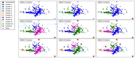
Figure 2.
Visualization of clustering results on a complex dataset using BIRCH.
With 4 and 5 clusters, the segmentation becomes more refined, capturing the natural groupings within the dataset. BIRCH effectively identifies cohesive regions, even in the presence of outliers, as indicated by isolated points in the scatterplot. The hierarchical nature of BIRCH is evident as it progressively organizes the data into clusters, maintaining balance and reducing computational complexity.
At higher cluster counts, such as 7, 8, and 9, the algorithm demonstrates its capacity to detect smaller, more localized clusters. However, this can lead to over-segmentation, where naturally cohesive groups are divided into sub-clusters. The presence of outliers remains well-managed, with some points clearly designated as noise. Overall, BIRCH shows its strength in clustering data hierarchically, balancing efficiency and accuracy, especially for datasets with varying densities and outliers.
Figure 3 demonstrates the progression of the Divisive Clustering algorithm as it separates the data into an increasing number of clusters, from 1 to 9. Initially, with a single cluster, all data points are grouped together, ignoring any inherent structure in the data. This provides no meaningful segmentation and highlights the starting point of the divisive hierarchical approach.
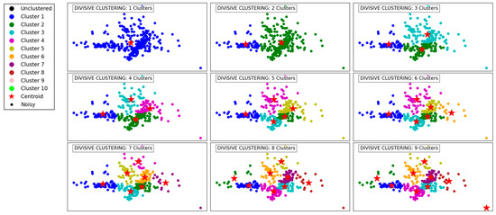
Figure 3.
Visualization of clustering results on a complex dataset using Divisive Clustering.
As the number of clusters increases to 2 and 3, the algorithm begins to partition the data into distinct groups based on its inherent structure. These initial divisions effectively segment the data into broad regions, capturing the overall distribution while maintaining cohesion within the clusters.
With 4 to 6 clusters, the algorithm refines these groupings further, identifying smaller clusters within the larger ones. This refinement captures finer details in the dataset’s structure, ensuring that densely populated areas are segmented appropriately. At this stage, Divisive Clustering demonstrates its ability to split clusters hierarchically, providing meaningful separations while maintaining a logical hierarchy.
At higher cluster counts, such as 7 to 9, the algorithm continues to divide existing clusters into smaller subgroups. This leads to a granular segmentation, effectively capturing subtle variations within the data. However, as the number of clusters increases, there is a risk of over-segmentation, where cohesive clusters are fragmented into smaller groups. Despite this, the algorithm handles outliers effectively, ensuring that isolated points are not erroneously grouped with larger clusters. Overall, Divisive Clustering effectively balances granularity and cohesion, making it well-suited for hierarchical data exploration.
Figure 4 illustrates the performance of the DBSCAN algorithm under varying eps and min_samples parameter configurations. DBSCAN’s ability to detect clusters of varying densities and its handling of noise is evident in the results.

Figure 4.
Visualization of clustering results on a complex dataset using DBSCAN.
With a small eps of 0.05 and min_samples set to 1, the algorithm identifies a large number of clusters (214), as the tight neighborhood criterion captures even minor density variations. This leads to over-segmentation and a significant amount of noise classified as individual clusters, reducing the interpretability of the results. Increasing min_samples to 3 under the same eps reduces the number of clusters (24) by merging smaller groups, though many data points remain unclustered. At min_samples 9, no clusters are identified, as the eps is too restrictive to form valid clusters.
When eps is increased to 0.1, the algorithm becomes less restrictive, capturing larger neighborhoods. For min_samples 1, the number of clusters decreases to 126, reflecting better grouping of data points. At min_samples 3, the results improve further, with fewer clusters (20) and more cohesive groupings. However, at min_samples 9, only 4 clusters are detected, with many points treated as noise.
With the largest eps value of 0.3, the algorithm identifies very few clusters, as the larger neighborhood radius groups most points into a few clusters. At min_samples 1, only 17 clusters are found, indicating over-generalization. For min_samples 3, the clusters reduce to 3, with most noise eliminated. Finally, at min_samples 9, only 2 clusters remain, demonstrating high consolidation but potentially missing finer details.
In summary, DBSCAN’s clustering performance is highly sensitive to eps and min_samples. Smaller eps values capture local density variations, leading to over-segmentation, while larger values risk oversimplifying the data. Higher min_samples values improve robustness by eliminating noise but can under-cluster sparse regions. The results highlight DBSCAN’s flexibility but emphasize the importance of parameter tuning for optimal performance.
Figure 5 demonstrates the performance of the OPTICS algorithm under varying min_samples and eps parameters. OPTICS, known for its ability to detect clusters of varying densities and hierarchical structures, shows its versatility and sensitivity to parameter adjustments.
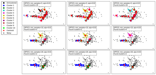
Figure 5.
Visualization of clustering results on a complex dataset using OPTICS.
For min_samples set to 5 and eps varying from 0.01 to 0.03, the algorithm identifies a relatively large number of clusters. At eps = 0.01, 19 clusters are detected, capturing fine density variations. As eps increases to 0.02 and 0.03, the number of clusters decreases slightly to 18 and 16, respectively. This reflects OPTICS’ tendency to merge smaller clusters as the threshold for cluster merging becomes more lenient. Despite this reduction, the algorithm still captures intricate cluster structures and maintains a high level of detail.
When min_samples increases to 10, the number of clusters decreases significantly. At eps = 0.01, only 5 clusters are found, reflecting stricter density requirements for forming clusters. As eps increases to 0.02 and 0.03, the cluster count further decreases to 5 and 4, respectively, with some finer details being lost. This highlights the impact of min_samples in reducing noise sensitivity but at the cost of losing smaller clusters.
For min_samples set to 20, the clustering results are highly simplified. Across all eps values, only 2 clusters are consistently detected, indicating a significant loss of detail and overgeneralization. While this reduces noise and improves cluster compactness, it risks oversimplifying the dataset and merging distinct clusters.
Overall, the results show that OPTICS performs well with low min_samples and small eps values, capturing fine-grained density variations and producing detailed cluster structures. However, as these parameters increase, the algorithm shifts towards merging clusters and simplifying the structure, which may lead to a loss of critical information in datasets with complex density variations. These findings emphasize the importance of careful parameter tuning to balance detail retention and noise reduction.
Figure 6 illustrates the performance of the Mean Shift clustering algorithm applied to the dataset, with varying bandwidth values from 0.1 to 5. Mean Shift is a non-parametric clustering method that groups data points based on the density of data in a feature space. The bandwidth parameter, which defines the kernel size used to estimate density, plays a critical role in determining the number and quality of clusters.
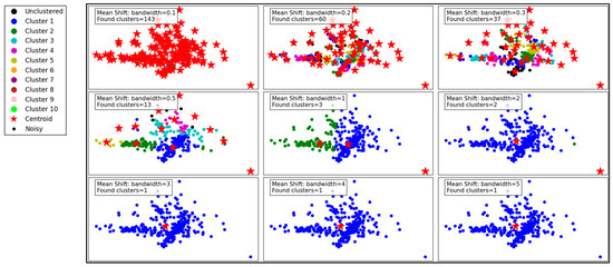
Figure 6.
Visualization of clustering results on a complex dataset using Mean Shift.
At a small bandwidth of 0.1, the algorithm detects 143 clusters, indicating a high sensitivity to local density variations. This results in many small clusters, capturing fine details in the dataset. However, such granularity may lead to over-segmentation, with clusters potentially representing noise rather than meaningful groupings. As the bandwidth increases to 0.2 and 0.3, the number of clusters decreases to 60 and 37, respectively. The algorithm begins merging smaller clusters, creating a more structured and meaningful segmentation while still retaining some level of detail.
With a bandwidth of 0.5, the cluster count drops sharply to 13, showing a significant reduction in granularity. The clusters become larger and less detailed, which may improve computational efficiency but risks oversimplifying the dataset. As the bandwidth continues to increase to 1 and beyond (e.g., 2, 3, 4, and 5), the number of clusters reduces drastically to 2 or even 1. At these high bandwidths, the algorithm generalizes heavily, resulting in overly simplistic cluster structures. This can lead to the loss of critical information and may render the clustering ineffective for datasets requiring fine-grained analysis.
In summary, the Mean Shift algorithm’s clustering performance is highly dependent on the bandwidth parameter. While smaller bandwidths allow for detailed and fine-grained clustering, they may result in over-segmentation and sensitivity to noise. Larger bandwidths improve generalization and computational efficiency but at the cost of significant loss of detail and potential oversimplification. Optimal bandwidth selection is essential to balance the trade-off between capturing meaningful clusters and avoiding over-generalization.
Figure 7 demonstrates the performance of the GMM clustering algorithm, evaluated across different numbers of components, ranging from 1 to 9. The GMM is a probabilistic model that assumes data are generated from a mixture of several Gaussian distributions, making it flexible for capturing complex cluster shapes. For the purpose of compression and vector quantization, each data point must be assigned to a single cluster, whether in the GMM or BGMM. To accomplish this, we adopt a hard assignment approach, where each point is assigned to the cluster with the highest probability, effectively selecting the most likely cluster based on maximum likelihood estimation.
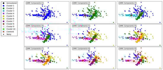
Figure 7.
Visualization of clustering results on a complex dataset using the GMM.
With a single component, the GMM produces a single, undifferentiated cluster, resulting in poor segmentation. All data points are grouped together, reflecting the model’s inability to distinguish underlying structures in the dataset. As the number of components increases to 2 and 3, the algorithm begins to form meaningful clusters, capturing distinct groupings in the data. However, overlapping clusters are still evident, indicating limited separation.
At 4 components, the clustering becomes more refined, and distinct patterns start emerging. The data points are grouped more accurately into cohesive clusters, demonstrating the ability of the GMM to model underlying structures. As the number of components increases to 5, 6, and 7, the algorithm continues to improve in capturing finer details and separating overlapping clusters. This results in a more accurate representation of the dataset, as observed in the clearer segmentation of the clusters.
By 8 and 9 components, the clustering is highly granular, with minimal overlap between clusters. However, the increased number of components may lead to overfitting, where the algorithm begins to model noise as separate clusters. This trade-off highlights the importance of carefully selecting the number of components to balance accuracy and generalizability.
In summary, the GMM effectively models the dataset’s underlying structure, with improved clustering performance as the number of components increases. However, excessive components can lead to overfitting, underscoring the need for optimal parameter selection. This makes the GMM a versatile and robust choice for applications requiring probabilistic clustering.
Figure 8 illustrates the clustering performance of the BGMM clustering algorithm across a range of component counts from 2 to 10. The BGMM, unlike GMM, incorporates Bayesian priors to determine the optimal number of components, providing a probabilistic framework for clustering. This makes the BGMM robust to overfitting, as it naturally balances the trade-off between model complexity and data representation.
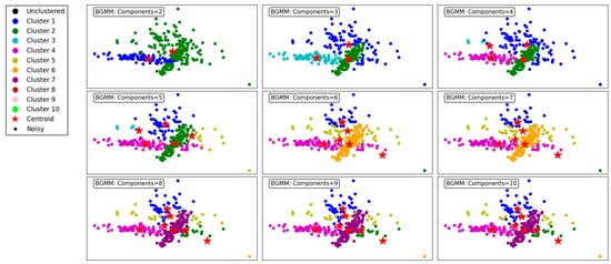
Figure 8.
Visualization of clustering results on a complex dataset using the BGMM.
At the lower component counts (2 to 3 components), the BGMM effectively identifies broad clusters in the dataset. For 2 components, the algorithm forms two distinct clusters, offering a coarse segmentation of the data. Increasing the components to 3 enhances granularity, with the addition of a third cluster capturing finer details within the dataset.
As the number of components increases to 4, 5, and 6, the BGMM achieves progressively finer segmentation, forming clusters that better align with the underlying data structure. Each additional component introduces greater specificity in capturing subgroups within the data, reflected in well-defined clusters. The transitions between clusters are smooth, indicating the algorithm’s ability to probabilistically assign points to clusters, even in overlapping regions.
From 7 to 9 components, the BGMM continues to refine the clustering process, but the benefits of additional components start to diminish. At 9 and 10 components, the model begins to overfit, with some clusters capturing noise or forming redundant groups. Despite this, the clusters remain relatively stable, showcasing the BGMM’s ability to avoid drastic overfitting compared to the GMM.
In conclusion, the BGMM demonstrates robust clustering performance across varying component counts. While the algorithm effectively captures complex data structures, it benefits from the Bayesian prior that discourages excessive components. This makes the BGMM particularly suited for scenarios where a balance between precision and generalizability is crucial. Figure 8 emphasizes the importance of selecting an appropriate number of components to maximize clustering efficiency and accuracy.
Figure 9 demonstrates the clustering results of the CLIQUE algorithm under varying grid sizes, showcasing its performance and adaptability. At a grid size of 1, no clusters are detected, which indicates that the granularity is too coarse to capture meaningful groupings in the dataset. As the grid size increases to 2 and 3, the algorithm begins to detect clusters, albeit sparingly, with 1 and 4 clusters identified, respectively. This improvement in cluster detection shows that a finer grid allows the algorithm to better partition the space and identify denser regions.
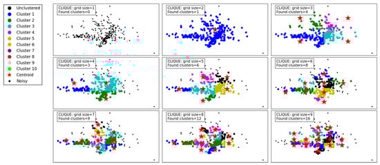
Figure 9.
Visualization of clustering results on a complex dataset using CLIQUE.
From grid size 4 to 6, there is a steady increase in the number of clusters found, reaching up to 8 clusters. The results reveal that moderate grid sizes provide a balance between capturing meaningful clusters and avoiding excessive noise or fragmentation in the data. Notably, the identified clusters at these grid sizes appear well-separated and align with the data’s inherent structure.
For larger grid sizes, such as 7 to 9, the number of clusters continues to grow, with up to 16 clusters detected. However, these finer grids risk over-partitioning the data, potentially splitting natural clusters into smaller subgroups. While the increase in clusters reflects a more detailed segmentation of the data, it might not always represent the most meaningful groupings, especially in practical applications.
Overall, the CLIQUE algorithm demonstrates its ability to adapt to different grid sizes, with the grid size playing a critical role in balancing cluster resolution and interpretability. Lower grid sizes result in the under-detection of clusters, while excessively high grid sizes may lead to over-fragmentation. Moderate grid sizes, such as 4 to 6, seem to strike the optimal balance, capturing the data’s underlying structure without overcomplicating the clustering.
5. Compression and Decompression Framework Using Clustering Techniques and Vector Quantization
Image compression using clustering techniques leverages the principle of grouping similar data points (pixels or blocks of pixels) into clusters, each represented by a centroid. The process is divided into two main phases: compression and decompression, each involving several steps.
5.1. Compression Phase
The compression phase aims to reduce the image’s size by representing groups of similar pixel values with a representative centroid (Figure 10). This phase involves the following detailed steps:

Figure 10.
Image compression using clustering techniques.
- ○
- The input image is first converted into a numerical format, typically a three-dimensional array for RGB images. If needed, the image can be converted to grayscale for simplicity (channels’ separation). To ensure compatibility with clustering algorithms, the image is divided into non-overlapping blocks of a predefined size (e.g., 2 × 2 or 4 × 4).
- ○
- Images whose dimensions are not divisible by the block size are zero-padded to ensure uniform block processing. Then, each block is flattened into a one-dimensional vector, forming the dataset for clustering.
- ○
- The data from different image channels are not concatenated into a single vector. Instead, clustering is performed independently for each channel, ensuring that color information is processed separately to preserve the structural integrity of the image.
- ○
- A suitable clustering algorithm is selected (e.g., K-Means, DBSCAN, GMM, etc.). The number of clusters or other algorithm-specific parameters (e.g., grid size for CLIQUE, eps for DBSCAN, etc.) are defined. The goal is to minimize intra-cluster differences and maximize inter-cluster differences.
- ○
- Each block vector is assigned to the nearest cluster based on a similarity metric (e.g., Euclidean distance). The cluster is represented by its centroid, which is a vector that minimizes the distance to all members of the cluster. In techniques like K-Means, centroids are iteratively updated until convergence. Grid-based methods (e.g., CLIQUE) use predefined grid structures to group blocks.
- ○
- The centroids, which represent the compressed version of the blocks, are quantized into a fixed range (e.g., 0–255 for image pixel values). This step ensures compatibility with image reconstruction.
- ○
- Each block in the original image is replaced with the index of the centroid to which it belongs. This mapping is saved in an index table. Together, the centroid values and index table form the compressed representation of the image.
- ○
- The compressed file consists of two main components: the centroid table and the index table, both stored in a binary format. To further reduce the size, the compressed data (centroid table and index table) are processed using LZMA (Lempel–Ziv–Markov Chain Algorithm), a high-ratio lossless compression method. LZMA effectively compresses repetitive patterns in the index table and centroid values by utilizing dictionary-based compression and advanced entropy coding. The output is a highly compact binary file that contains the LZMA-compressed centroid and index data.
5.2. Decompression Phase
The decompression phase reconstructs the original image (or its approximate version) from the compressed data (Figure 11). It involves the following steps:
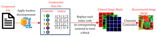
Figure 11.
Image decompression using centroids of clustering techniques.
- ○
- The compressed file is read and passed through LZMA to extract the centroid and index tables. These represent the core information required for reconstruction.
- ○
- Each block in the decompressed image is reconstructed by replacing the index in the index table with the corresponding centroid vector from the centroid table. The centroid vector is reshaped back to its original block dimensions (e.g., 2 × 2 or 4 × 4).
- ○
- The reconstructed blocks are reassembled into their original positions to form the decompressed image. This step restores the spatial structure of the image.
- ○
- Any artifacts introduced during compression (e.g., boundary mismatches between blocks) may be reduced using optional smoothing or filtering techniques. However, this step is not always necessary, depending on the clustering method used.
6. Quality Assessment Metrics for Image Compression
Evaluating the quality of image compression is critical to balancing the trade-off between reducing file size and preserving visual fidelity. This section provides a detailed explanation of three key metrics: compression ratio (CR), bits per pixel (BPP), and structural similarity index (SSIM). Each metric quantifies different aspects of compression performance, including file size reduction, efficiency, and perceived image quality.
6.1. Compression Ratio (CR)
The compression ratio (CR) measures how much the original image has been compressed [8]. It is the ratio of the original image size to the compressed image size, expressed mathematically as:
where
- : Size of the original image file (in bytes);
- : Size of the compressed image file (in bytes).
A higher CR indicates a greater reduction in file size, which is desirable for applications where storage or bandwidth constraints are a priority.
6.2. Bits per Pixel (BPP)
Bits per pixel (BPP) quantifies the average number of bits used to represent each pixel in the compressed image [8]. It reflects the efficiency of compression in terms of information density and is calculated as:
where
- : Size of the compressed image file (in bytes);
- : Height of the image (in pixels);
- : Width of the image (in pixels);
- The factor 8 converts bytes to bits.
BPP is inversely proportional to CR, meaning that as the compression ratio increases, the bits per pixel decrease. A lower BPP signifies a higher degree of compression efficiency, meaning fewer bits are used to encode the image without significantly degrading its quality.
6.3. Structural Similarity Index (SSIM)
SSIM is a perceptual metric that quantifies the visual similarity between the original and compressed images [8]. Unlike pixel-wise comparisons (e.g., Mean Squared Error or Peak Signal-to-Noise Ratio), SSIM considers structural information, luminance, and contrast. It is defined as:
where
- and : Corresponding image patches from the original and compressed images, respectively;
- and : Mean intensities of and ;
- and : Variances of and ;
- : Covariance of and ;
- and : Small constants to stabilize the division when the denominator is close to zero.
To obtain the SSIM for the entire image, a sliding window approach is used, where SSIM is calculated over multiple overlapping patches across the image. The final SSIM value is then determined by averaging the SSIM scores of all patches. A higher SSIM value, closer to 1, indicates greater similarity between the original and compressed images, suggesting minimal perceptual degradation.
7. Comprehensive Performance Analysis of Clustering Techniques in Image Compression
This section presents the performance evaluation of various clustering-based image compression techniques. Each method was applied to compress images using the proposed framework, followed by quantitative and qualitative assessments of the reconstructed images. Metrics such as CR, BPP, and SSIM were calculated to gauge the trade-offs between compression efficiency and image quality. Block sizes of 2 × 2, 4 × 4, 8 × 8, and 16 × 16 were applied across different clustering techniques to evaluate their impact on compression performance. However, some methods, such as BIRCH, DBSCAN, OPTICS, and CLIQUE, were only experimented with smaller block sizes (2 × 2, 4 × 4) due to the significant memory resources they require, which were not available on our hardware. The results highlight the strengths and limitations of each method, offering insights into their suitability for different compression scenarios. The findings are summarized and analyzed in the subsequent subsections.
The initial experimental results for image compression presented in this section utilized the widely recognized “Peppers” image (Figure 12) obtained from the Waterloo dataset [59], a benchmark resource for image processing research.
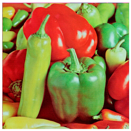
Figure 12.
Peppers image from the Waterloo dataset (512 × 512).
7.1. K-Means Clustering for Compression
Figure 13 illustrates the results of image compression using the K-Means clustering algorithm with different block sizes and numbers of clusters. We have implemented K-Means++ as an optimized strategy for centroid initialization to enhance clustering efficiency and improve convergence stability. Starting with the smallest block size of 2 × 2 pixels, the images exhibit high SSIM values, close to 1, indicating a strong similarity to the original image. This high SSIM is expected because the small block size allows for finer granularity in capturing image details. However, as the number of clusters increases from 31 to 255, there is a noticeable trade-off between CR and BPP. When the number of clusters is low, the CR is relatively high (14.14), but the BPP is low (1.70), indicating efficient compression. As the number of clusters increases, the CR decreases significantly (6.13), while the BPP increases to 3.91. This indicates that the image quality is maintained at the cost of compression efficiency, as more clusters mean more distinct pixel groups, which reduces the compression ratio.
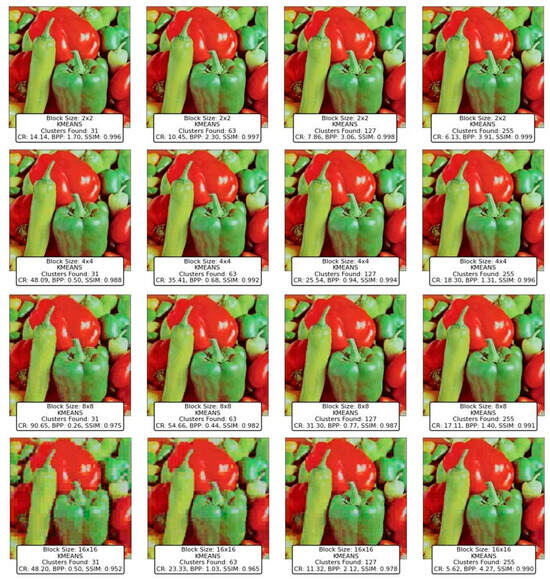
Figure 13.
Results of K-Means clustering for compressing the Peppers image with varying numbers of clusters and block sizes.
When the block size is increased to 4 × 4 pixels, the reconstructed images still maintain high SSIM values, though slightly lower than with the 2 × 2 block size. This decrease in SSIM is due to the larger block size capturing less fine detail, making the reconstruction less accurate. The compression ratio improves significantly, reaching as high as 48.09 when using 31 clusters. However, as with the 2 × 2 block size, increasing the number of clusters leads to a reduction in the compression ratio (down to 18.30 with 255 clusters) and an increase in BPP, indicating that more data are needed to preserve the image quality. The images with 4 × 4 blocks and a higher number of clusters show a good balance between compression and quality, making this configuration potentially optimal for certain applications where moderate image quality is acceptable with better compression efficiency.
The 8 × 8 block size introduces more noticeable artifacts in the reconstructed images, particularly as the number of clusters increases. Although the compression ratio remains high, the SSIM values start to drop, especially as we move to higher cluster counts. The BPP values are also lower compared to smaller block sizes, indicating higher compression efficiency. However, this comes at the expense of image quality, as larger blocks are less effective at capturing the fine details of the image, leading to a more pixelated and less accurate reconstruction. The trade-off is evident here: while the compression is more efficient, the image quality suffers, making this configuration less desirable for applications requiring high visual fidelity.
Finally, the largest block size of 16 × 16 pixels shows a significant degradation in image quality. The SSIM values decrease noticeably, reflecting the loss of detail and the introduction of more visible artifacts. The compression ratios are very high, with a maximum CR of 48.25, but the images appear much more pixelated and less recognizable compared to those with smaller block sizes. This indicates that while large block sizes are highly efficient for compression, they are not suitable for scenarios where image quality is a priority. The BPP values also vary significantly, with lower cluster counts resulting in very low BPP, but as the number of clusters increases, the BPP rises, indicating that the image quality improvements come at the cost of less efficient compression.
In summary, Figure 13 demonstrates that the K-Means clustering algorithm’s effectiveness for image compression is highly dependent on the choice of block size and the number of clusters. Smaller block sizes with a moderate number of clusters offer a good balance between image quality and compression efficiency, making them suitable for applications where both are important. Larger block sizes, while more efficient in terms of compression, significantly degrade image quality and are less suitable for applications requiring high visual fidelity. The results highlight the need to carefully select these parameters based on the specific requirements of the application, whether it prioritizes compression efficiency, image quality, or a balance of both.
7.2. BIRCH Clustering for Compression
Figure 14 displays a series of reconstructed images using the BIRCH clustering algorithm applied to image compression. Starting with the block size of 2 × 2, the images exhibit varying levels of quality depending on the threshold and branching factor used. For a block size of 2 × 2, with a threshold of 0.1 and a branching factor of 10, the SSIM values range around 0.219 to 0.241, indicating a dissimilarity to the original image. The CR is low, around 1.75 to 1.85, and the BPP is high, ranging from 12.94 to 13.74, reflecting a lower compression efficiency and a higher level of detail retention. However, as the threshold increases to 0.5, while keeping the branching factor constant at 10, the SSIM decreases significantly, with values dropping to as low as 0.163 to 0.184, indicating a deterioration in image quality. Despite this, the CR slightly improves, suggesting that more aggressive compression is taking place at the expense of image quality.
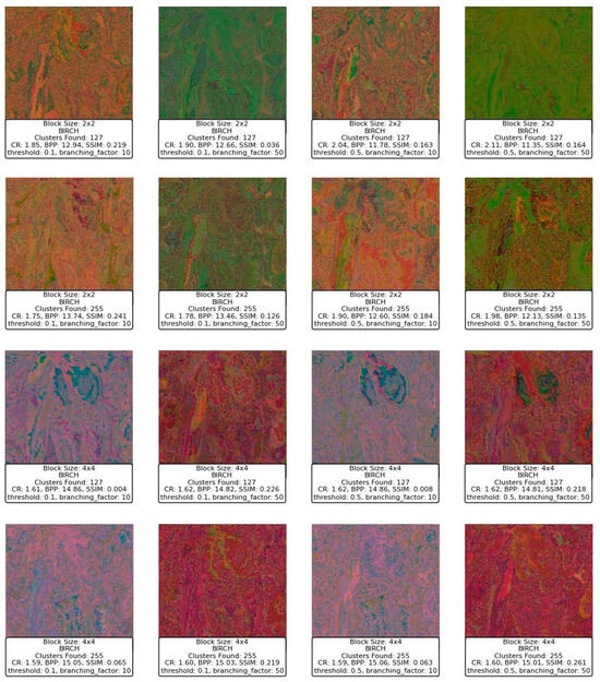
Figure 14.
Results of BIRCH clustering for compressing the Peppers image with varying threshold, branching factor, and block sizes.
When increasing the branching factor to 50, the SSIM values decrease even further, especially for the higher threshold of 0.5, where the SSIM drops to 0.036 and 0.126. This indicates that the reconstructed images lose significant detail and structure, becoming almost unrecognizable. The BPP remains high, suggesting that although a large amount of data are being retained, they are not contributing positively to the image quality. The CR does not show significant improvement, which suggests that the BIRCH algorithm with these parameters might not be efficiently clustering the blocks in a way that balances compression with quality.
Moving to a block size of 4 × 4, the images generally show a deterioration in SSIM compared to the smaller block size, with SSIM values dropping to below 0.1 in several cases, particularly when the threshold is set to 0.5. The BPP shows slight improvements in some cases, but the SSIM remains relatively low, indicating that even though more bits are used per pixel, the quality does not improve and, in some cases, worsens significantly. For example, with a threshold of 0.5 and a branching factor of 50, the SSIM is 0.219, which is slightly better than other configurations with the same block size but still low.
In summary, the BIRCH algorithm appears to struggle with balancing compression and image quality in this context, especially with larger block sizes and higher thresholds. The SSIM values suggest that as the threshold and branching factor increase, the algorithm fails to maintain structural similarity, leading to poor-quality reconstructions. The CR and BPP metrics indicate that while compression is occurring, it is not efficiently capturing the important details needed to reconstruct the image well. This suggests that BIRCH may not be the optimal clustering method for this type of image compression, particularly with larger block sizes and more aggressive parameter settings.
7.3. Divisive Clustering for Compression
Figure 15 presents the results of applying the Divisive Clustering method to compress and reconstruct an image. At a block size of 2 × 2, the method preserves high structural similarity (SSIM close to 1) across different cluster sizes. However, increasing the number of clusters from 31 to 255 leads to a decrease in compression ratio (CR) from 14.22 to 6.58, while the bits per pixel (BPP) increases, indicating a trade-off between compression and quality.

Figure 15.
Results of Divisive Clustering for compressing the Peppers image with varying numbers of clusters and block sizes.
For the 4 × 4 block size, the CR improves significantly, reaching 49.64 with 31 clusters, demonstrating the method’s efficiency in compressing images at larger block sizes. However, increasing the number of clusters to 255 reduces the CR to 18.30, while SSIM remains high, showing that Divisive Clustering can maintain good image quality at this level. The method continues to perform well for 8 × 8 blocks, achieving a peak CR of 93.01, but SSIM slightly drops as clusters increase. At a 16 × 16 block size, the method reaches its highest CR of 48.66 with 31 clusters, but image quality degrades slightly with lower SSIM. However, increasing the number of clusters to 255 partially restores image quality while sacrificing compression efficiency.
Overall, Divisive Clustering and K-Means exhibit similar trends in compression performance and image quality, demonstrating their shared characteristics as partitioning-based clustering techniques.
7.4. DBSCAN and OPTICS Clustering for Compression
Figure 16 and Figure 17 represent the results of image compression using two clustering techniques: DBSCAN and OPTICS. Both methods are designed to identify clusters of varying densities and can handle noise effectively, which makes them particularly suitable for applications where the underlying data distribution is not uniform. However, the results demonstrate distinct differences in how each method processes the image blocks, especially under varying parameter settings. It is important to note that blocks that do not belong to any identified cluster are classified as noise and are assigned unique centroids. This approach accounts for the significantly higher number of clusters observed in certain cases, as each noisy block is treated as an independent entity.
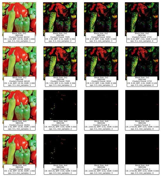
Figure 16.
Results of DBSCAN clustering for compressing the Peppers image with varying eps, min_samples, and block sizes.
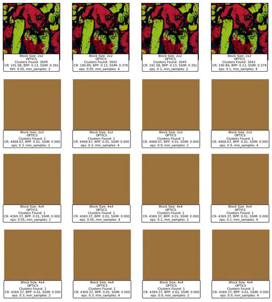
Figure 17.
Results of OPTICS clustering for compressing the Peppers image with varying eps, min-samples, and block sizes.
DBSCAN’s performance across different block sizes and parameter configurations shows a stark contrast in image quality and compression metrics. At smaller block sizes (2 × 2), DBSCAN tends to find a very high number of clusters when the eps parameter is low, such as 0.1, and min_samples is set to 1. This results in an extremely high cluster count (e.g., 46,142 clusters found), but this comes at the cost of poor CR and BPP, as seen in Figure 16. The SSIM value remains high, indicating a good structural similarity, but the practical usability of such a high cluster count is questionable, as it results in high computational overhead and potentially overfitting the model to noise.
As the eps value increases (e.g., from 0.1 to 0.3) and min_samples rises, the number of clusters decreases significantly, which is accompanied by a drop in SSIM and an increase in CR and BPP. For instance, when eps is 0.3 and min_samples is 4, DBSCAN produces far fewer clusters, leading to much more compressed images but with significantly degraded quality, as evidenced by the low SSIM values. At larger block sizes (e.g., 4 × 4), DBSCAN’s performance diminishes drastically, with the number of clusters dropping to nearly zero in some configurations. This results in almost no useful information being retained in the image, reflected in the SSIM dropping to zero, indicating a total loss of image quality.
OPTICS, which is similar to DBSCAN but provides a more nuanced approach to identifying clusters of varying densities, shows a different pattern in image processing. Like DBSCAN, the effectiveness of OPTICS is highly dependent on its parameters (eps and min_samples). Figure 17 shows that, regardless of the block size, OPTICS identifies a very small number of clusters (often just 1), especially when eps is set to 0.3 and min_samples is varied. This leads to extremely high CR and very low BPP, but at the cost of significant image distortion and loss, as seen in the brownish, almost entirely abstract images produced.
One notable observation is that OPTICS tends to retain minimal useful image information even when identifying a single cluster, leading to highly compressed images with very high CR but nearly zero SSIM. This suggests that OPTICS, under these settings, compresses the image to the point of obliterating its original structure, making it less suitable for tasks where preserving image quality is essential.
When comparing DBSCAN and OPTICS, it becomes clear that while both methods aim to find clusters in data, their behavior under similar parameter settings leads to vastly different results. DBSCAN’s flexibility in finding a large number of small clusters can either be an advantage or a hindrance depending on the parameter configuration, whereas OPTICS, in this particular case, consistently produces fewer clusters with more significant compression but at the cost of image quality. For instance, both techniques perform poorly with larger block sizes, but DBSCAN’s sensitivity to eps and min_samples allows for more granular control over the number of clusters and the resulting image quality. On the other hand, OPTICS, while theoretically offering advantages in handling varying densities, does not seem to leverage these advantages effectively in this context, leading to overly aggressive compression. The images produced by DBSCAN with lower eps values and small min_samples show that it can maintain a relatively high SSIM while achieving reasonable compression, although this comes with a high computational cost due to the large number of clusters. In contrast, OPTICS, even with different settings, fails to preserve the image structure, resulting in images that are visually unrecognizable.
7.5. Mean Shift Clustering for Compression
Figure 18 presents the results of image compression using the Mean Shift clustering algorithm across different block sizes and bandwidth parameters. At the smallest block size (2 × 2), the clustering process identifies an extremely high number of clusters, with values exceeding 46,000 clusters for bandwidth values of 0.1 and 0.3. Despite the large number of clusters, the compression ratio (CR) is exceptionally low, around 1.36 to 2.12, which suggests that the method is ineffective at reducing image storage size. However, the SSIM remains at 1.000, indicating an almost perfect reconstruction of the original image. The bits per pixel (BPP) remains high, indicating that the compression is not optimized for efficiency.
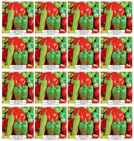
Figure 18.
Results of Mean Shift clustering for compressing the Peppers image with varying bandwidth and block sizes.
As the block size increases to 4 × 4, 8 × 8, and 16 × 16, a similar trend is observed where the number of clusters remains high, with minimal improvement in CR. The CR slightly increases from 1.48 (4 × 4) to 1.62 (16 × 16), but these values remain significantly lower compared to other clustering methods like K-Means or Divisive Clustering. This suggests that Mean Shift fails to provide effective compression because it tends to over-cluster image regions, leading to a high number of unique clusters that prevent substantial data reduction.
In conclusion, while Mean Shift preserves image quality perfectly (SSIM = 1.000), its compression efficiency is extremely poor. The high cluster count results in minimal data reduction, making it impractical for image compression. Unlike other methods that balance quality and compression, Mean Shift fails to achieve a desirable trade-off. Thus, it is not a viable option for practical image compression applications.
7.6. GMM and BGMM Clustering for Compression
Figure 19 and Figure 20 present the results of compressing an image using the GMM and BGMM clustering methods. For a block size of 2 × 2, both the GMM and BGMM achieve high compression ratios at lower cluster counts, with the GMM reaching a CR of 12.63 and BGMM at 12.07 with 31 clusters. As the cluster count increases to 255, the CR drops while SSIM improves, showing a trade-off between compression efficiency and quality. The highest SSIM values for both methods remain above 0.98, indicating strong image fidelity.
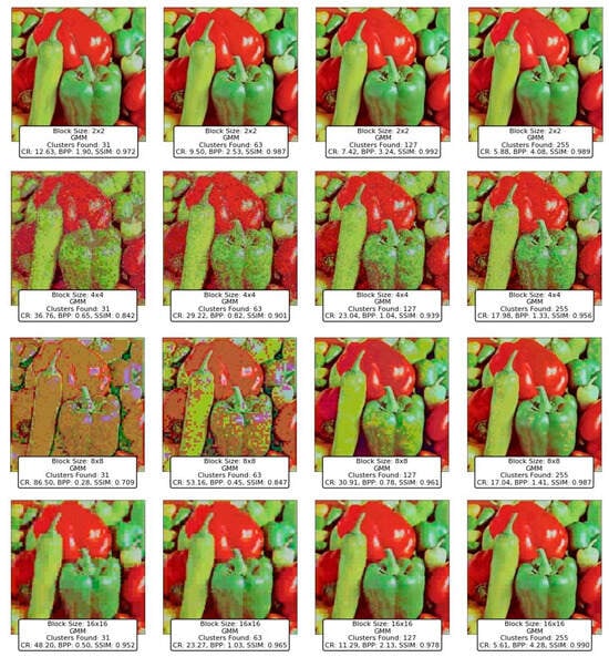
Figure 19.
Results of GMM clustering for compressing the Peppers image with varying numbers of clusters and block sizes.
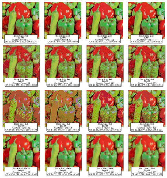
Figure 20.
Results of BGMM clustering for compressing the Peppers image with varying numbers of clusters and block sizes.
With a 4 × 4 block size, compression ratios improve significantly, especially with lower cluster counts. Both methods reach CR values above 30 when using 31 clusters, while higher cluster counts lead to better SSIM at the cost of reduced compression efficiency. At 127 clusters, the GMM achieves a CR of 23.04 and an SSIM of 0.939, while the BGMM records 26.62 and 0.906, respectively.
At an 8 × 8 block size, compression ratios further increase, with the GMM reaching 86.50 and the BGMM 89.99 for 31 clusters. However, the SSIM remains relatively low in this setting. As clusters increase, SSIM improves, peaking at 0.987 for the GMM and 0.921 for BGMM at 255 clusters. This highlights that more clusters are necessary for maintaining image quality when using larger blocks.
For a 16 × 16 block size, maximum compression efficiency is achieved, with CR values exceeding 40 for low cluster counts. However, SSIM is initially lower due to larger data blocks capturing less detail. With 31 clusters, the GMM records a CR of 48.20 and SSIM of 0.952, while the BGMM achieves 49.16 and 0.950. At 255 clusters, both methods reach SSIM values above 0.96, providing high-quality reconstruction but at lower compression efficiency.
Overall, both the GMM and BGMM perform nearly identically, with the BGMM slightly favoring compression efficiency at lower cluster counts. The results confirm that distribution-based methods can maintain strong image fidelity while achieving significant compression, making them suitable for balancing storage efficiency and visual quality.
7.7. CLIQUE Clustering for Compression
Figure 21 presents the results of the CLIQUE clustering method applied for image compression with varying grid sizes, ranging from 1 to 8.5. The block size used in all experiments is fixed at 2 × 2, and the grid size controls the number of clusters and consequently affects compression performance and quality. Since CLIQUE is a grid-based clustering method, unclustered blocks are reassigned to the nearest dense grid cell, ensuring continuity in the compressed representation while minimizing data loss.
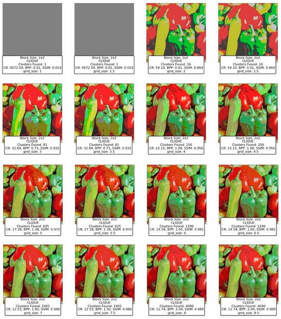
Figure 21.
Results of CLIQUE clustering for compressing the Peppers image with varying grid and block sizes.
For grid sizes 1.5 and 2.0, the algorithm identifies only 1 and 16 clusters, respectively. These settings result in poor visual quality, as evidenced by the low SSIM values (0.014 and 0.864, respectively) and the inability to retain structural details in the image. The CR values are exceptionally high (4572.59 and 59.10), but this comes at the cost of extreme data loss, as depicted by the highly distorted or gray images.
Increasing the grid size from 2.5 to 4.5 results in more clusters (81 to 256), which improves the image’s visual quality. The SSIM steadily increases, reaching 0.956 at a grid size of 4.5, indicating a good retention of structural similarity compared to the original image. Correspondingly, the CR values drop significantly (32.84 to 22.15), reflecting a more balanced trade-off between compression and quality. The images become visually more acceptable as the grid size increases, with better preservation of object edges and colors.
At grid sizes 5.0 to 6.0, the number of clusters increases drastically (625 and 1296), resulting in improved image quality. The SSIM values rise further (0.972 to 0.981), indicating near-perfect structural similarity. The BPP also increases moderately (1.38 to 1.65), demonstrating a slight trade-off in compression efficiency. The images exhibit finer details and color fidelity is well-preserved, making these grid sizes suitable for high-quality compression scenarios.
As the grid size increases from 6.5 to 8.5, the number of clusters grows exponentially (2401 to 4096). The SSIM approaches near-perfection (0.986 to 0.989), and the BPP increases significantly (1.92 to 2.04). These results reflect excellent image reconstruction quality with minimal perceptual differences from the original image. However, the CR values continue to decrease (12.53 to 11.74), highlighting the trade-off between compression efficiency and quality. These grid sizes are ideal for applications requiring minimal quality loss, even at the expense of reduced compression efficiency.
The performance of the CLIQUE method is highly dependent on the grid size, with a direct relationship between grid size and the number of clusters. Lower grid sizes result in fewer clusters, leading to higher compression ratios but significantly compromised image quality, as evidenced by low SSIM values and poor visual results. Medium grid sizes, such as 4.5 to 6.0, strike a balance between compression efficiency and image quality, maintaining good structural integrity while offering reasonable compression ratios. On the other hand, higher grid sizes (e.g., 6.5 to 8.5) generate more clusters, yielding near-perfect SSIM values and visually indistinguishable images from the original but at the cost of reduced compression efficiency.
7.8. Computational Efficiency Analysis
In this evaluation, all image compression techniques were applied using a fixed block size of 4 × 4 pixels. This uniform partitioning ensures consistency across different methods, allowing for a fair comparison of their computational efficiency. The experiments were conducted on a system with the following specifications:
- Processor: 11th Gen Intel® Core™ i7-11800H @ 2.30 GHz;
- Installed RAM: 32.0 GB;
- System Type: 64-bit operating system, x64-based processor;
- Operating System: Windows 11 Pro (Dev Version).
The results of Table 4 indicate significant variations in compression time among the techniques. CLIQUE exhibited the fastest performance, with the lowest processing time, making it the most efficient method in this study. K-Means followed with a relatively low computation time, reinforcing its suitability for real-time applications.
Table 4.
Compression and decompression time of different clustering methods.
Conversely, methods such as Mean Shift, GMM, and BGMM demonstrated considerably higher computational costs, likely due to their iterative nature and probabilistic modeling. OPTICS also showed a substantial runtime, reflecting its density-based approach’s complexity. Meanwhile, BIRCH, Divisive Clustering, and DBSCAN presented moderate execution times, balancing efficiency and effectiveness.
7.9. Discussion
The evaluation of the nine clustering techniques highlights the diverse strengths and limitations of each method in the context of image compression. Each technique offers unique trade-offs between compression efficiency, image quality, and computational complexity, making them suitable for different applications depending on the specific requirements.
K-Means stands out as a robust and versatile method for image compression, demonstrating a good balance between compression efficiency and image quality across various block sizes and cluster configurations. Its ability to produce consistent results with high SSIM values and moderate compression ratios makes it a strong candidate for applications requiring both visual fidelity and reasonable storage savings. However, its performance diminishes slightly with larger block sizes, where fine-grained image details are lost, leading to visible artifacts.
BIRCH, on the other hand, struggles to balance compression and quality, particularly with larger block sizes and higher thresholds. Its tendency to lose structural similarity at higher parameter settings indicates its limitations in preserving critical image features. While BIRCH may excel in other data clustering contexts, its application in image compression appears less effective compared to other techniques.
Divisive Clustering showcases excellent adaptability, particularly with smaller block sizes, where it maintains high SSIM values and reasonable compression ratios. As the block size increases, it achieves impressive compression efficiency with only a slight compromise in image quality. Its hierarchical nature enables it to provide granular control over the clustering process, making it well-suited for scenarios requiring a balance between compression and quality.
Density-based methods like DBSCAN and OPTICS highlight the challenges of applying these techniques to image compression. DBSCAN’s performance varies significantly with its parameters (eps and min_samples), often producing high SSIM values at the cost of computational overhead and impractical cluster counts. OPTICS, while theoretically advantageous for handling varying densities, shows limited effectiveness in this application, often leading to excessive compression at the expense of image structure. Both methods illustrate the importance of parameter tuning and the potential challenges of adapting density-based clustering for image compression.
Mean Shift emerges as a stable technique, particularly for smaller block sizes and lower bandwidth settings. Its non-parametric nature allows it to adapt well to the data, resulting in high SSIM values and low compression ratios. However, as block sizes increase, the sensitivity of Mean Shift to its bandwidth parameter diminishes, leading to less pronounced variations in results. This stability makes it an attractive option for applications where consistency across different settings is desirable.
The GMM and BGMM provide complementary perspectives on probabilistic clustering for image compression. The GMM demonstrates more pronounced changes in performance across block sizes and cluster counts, offering high compression ratios but at the cost of noticeable quality degradation for larger block sizes. In contrast, the BGMM delivers more consistent image quality with slightly higher BPP, making it a reliable choice for scenarios prioritizing visual fidelity over extreme compression efficiency.
Finally, CLIQUE, a grid-based clustering method, demonstrates the importance of balancing grid size with block size to achieve optimal results. While smaller grid sizes lead to significant compression, they often produce highly distorted images. Medium grid sizes strike a balance, maintaining reasonable compression ratios and good image quality, whereas larger grid sizes yield near-perfect SSIM values at the expense of reduced compression efficiency. CLIQUE’s grid-based approach offers a unique perspective, emphasizing the interplay between spatial granularity and compression performance.
In summary, the comparative analysis of these techniques underscores the necessity of selecting a clustering method tailored to the specific requirements of the application. Techniques like K-Means, Divisive Clustering, and BGMM excel in maintaining a balance between compression efficiency and image quality, making them suitable for general-purpose applications. Methods such as CLIQUE and Mean Shift provide specialized advantages, particularly when specific parameter configurations are carefully tuned. On the other hand, techniques like DBSCAN and OPTICS highlight the challenges of adapting density-based clustering to this domain, while BIRCH’s limitations in this context emphasize the importance of evaluating clustering methods in their intended use cases.
8. Validation of Compression Results Using CID22 Benchmark Dataset
The CID22 dataset [60] is a diverse collection of high-quality images specifically designed for evaluating image compression and other computer vision algorithms. It offers a wide range of visual content, including dynamic action scenes, intricate textures, vibrant colors, and varying levels of detail, making it an ideal choice for robust validation.
For this study, eight representative images were selected, as shown in Figure 22, covering diverse categories such as sports, mechanical objects, food, landscapes, macro photography, artwork, and medical images. This selection ensures comprehensive testing across different types of visual data, capturing various challenges like high-frequency details, smooth gradients, and complex patterns. The dataset’s diversity allows for a thorough assessment of the clustering-based compression techniques, providing insights into their performance across real-world scenarios.
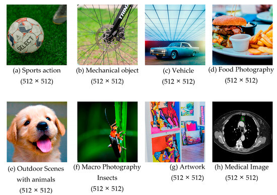
Figure 22.
Benchmark images from the CID22 dataset.
Figure 23a–h and Table 5 show the results of compressing the benchmark images using the nine clustering techniques, in addition to PNG and JPEG compressors. Table 5 highlights the consistently high SSIM values observed at higher compression ratios, demonstrating the effectiveness of the compression method in preserving image quality while achieving significant data reduction.


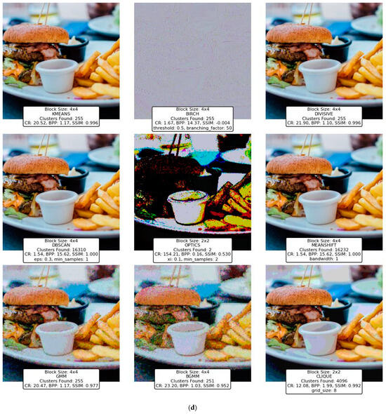


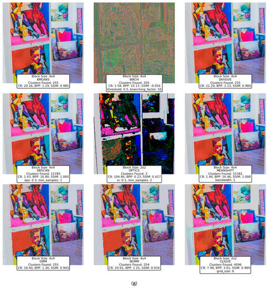
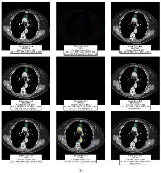
Figure 23.
Results of clustering-based compression for different types of images. (a) Sports action (b). Mechanical objects (c). Vehicle (d). Food photography (e). Outdoor scenes with animals (f). Macro photography (g). Artwork. (h). Medical image.
Table 5.
CR and SSIM metrics for clustering-based compression, PNG and JPEG.
K-Means consistently delivers a balanced performance across all image categories. For instance, in sports and vehicles, it achieves high CR values (27.95 and 27.05, respectively) while maintaining excellent SSIM values (0.996 and 0.997). This indicates its effectiveness in preserving structural details while achieving reasonable compression. However, for more intricate scenes, such as macro photography, the CR increases to 30.58, suggesting its adaptability for detailed data. Overall, K-Means achieves a good balance between compression efficiency and image quality, making it versatile for a variety of image types.
BIRCH exhibits low performance in both CR and SSIM across all image types. For example, in food photography and macro photography, it achieves SSIM values of −0.004 and −0.032, respectively, with CR values of 1.67 and 3.39. These results indicate significant quality loss and inefficiency in compression. The method struggles to adapt to the complexities of natural scenes or high-detail photography. BIRCH’s weak performance suggests it may not be suitable for image compression tasks where quality retention is critical.
Divisive Clustering achieves high CR and SSIM values across most categories, particularly in medical and vehicles, with CR values of 33.39 and 28.34 and SSIM values of 0.991 and 0.994, respectively. These results show that the method preserves image quality effectively while achieving efficient compression. For macro photography, it performs similarly well, achieving an SSIM of 0.996. Divisive Clustering emerges as one of the top-performing techniques, maintaining a balance between efficiency and visual quality.
DBSCAN’s performance is highly dependent on parameter settings and image content. It achieves perfect SSIM values (1.0) for several categories, such as food photography and vehicles, but at the cost of extremely low CR values (e.g., 1.43 for artwork). This indicates over-segmentation, leading to inefficiencies in practical compression. In outdoor scenes and artwork, the method shows reduced CR values but still retains high SSIM, demonstrating its adaptability for specific types of data. However, its tendency to overfit or underperform depending on parameter tuning makes it less reliable overall.
OPTICS performs poorly in terms of compression efficiency and image quality. For most categories, such as sports and food photography, it achieves very high CR values (159.73 and 154.21) but with significantly degraded SSIM values (0.414 and 0.530). The images reconstructed using OPTICS often exhibit severe distortions and fail to retain meaningful structural details. The method’s performance suggests it is not well-suited for image compression tasks where preserving visual quality is important.
Mean Shift shows significant limitations in terms of compression efficiency. Despite achieving perfect SSIM values (1.0) across several categories (e.g., sports, food photography, and vehicles), its CR values are consistently low (e.g., 1.50 to 2.91). This indicates poor compression efficiency, making Mean Shift unsuitable for practical image compression tasks where achieving a high CR is essential. While it preserves image quality well, its limited efficiency renders it a less favorable choice for real-world applications.
The GMM achieves a strong balance between compression and quality, particularly in vehicles and sports, with CR values of 24.44 and 18.21 and SSIM values of 0.978 and 0.981, respectively. However, it struggles slightly with macro photography, where SSIM drops to 0.933. While the GMM performs well overall, its performance is slightly less consistent compared to Divisive Clustering or K-Means. Nonetheless, it remains a strong option for applications requiring good compression and quality balance.
The BGMM exhibits stable performance across all categories, retaining higher CR values than GMM in most cases. For instance, in vehicles and macro photography, the BGMM achieves CR values of 28.88 and 29.27, respectively. The SSIM values are also competitive, with a maximum of 0.968 in vehicles.
CLIQUE emerges as a good-performing method, combining high compression efficiency with excellent quality retention. In sports and vehicles, it achieves CR values of 14.03 and 14.40 and SSIM values of 0.992. In macro photography, it maintains a strong balance, achieving an SSIM of 0.963 while maintaining a reasonable CR of 29.29. CLIQUE adapts well to a wide range of image complexities and demonstrates consistent performance, making it a strong competitor to K-Means and Divisive Clustering.
PNG consistently achieves low CR across all image categories, reinforcing its lossless nature. The CR values for PNG range from 1.38 for outdoor scenes to 4.80 for medical images, confirming that PNG prioritizes image quality preservation over compression efficiency.
JPEG provides significantly better compression than PNG, with a CR of 38.40 for macro photography, making it the most effective method in that category. It also performs well for sports action and outdoor scenes, both at 24.00, and for food photography at 21.33. However, JPEG does not always surpass clustering-based techniques, particularly for medical images, where it has a CR of 24.00 compared to CLIQUE’s 36.30.
In summary, K-Means, Divisive Clustering, and CLIQUE stand out as the most reliable clustering methods for image compression, offering consistent performance across diverse image types. These methods effectively balance compression efficiency (high CR) and image quality (high SSIM), making them suitable for a wide range of applications. GMM and BGMM also provide good results but may require careful parameter tuning to achieve optimal performance. Mean Shift, despite its ability to retain image quality, is limited by poor compression efficiency, making it unsuitable for most compression scenarios. BIRCH, DBSCAN, and OPTICS exhibit significant limitations in either quality retention or compression efficiency, rendering them less favorable for practical applications.
9. Conclusions and Future Research Directions
Image compression is a crucial aspect of digital media management, enabling efficient storage, transmission, and accessibility of large-scale image data. With the growing demand for high-quality visual content in applications ranging from healthcare to entertainment, the development of effective compression methods is more important than ever. Clustering techniques offer a promising approach to image compression by grouping pixel data based on similarity, allowing for reduced storage requirements while maintaining structural fidelity. In this paper, we systematically evaluated nine clustering techniques—K-Means, BIRCH, Divisive Clustering, DBSCAN, OPTICS, Mean Shift, GMM, BGMM, and CLIQUE—for their performance in compressing images.
The findings highlight the versatility and efficacy of clustering-based approaches, with K-Means, Divisive Clustering, and CLIQUE emerging as the most reliable methods. K-Means demonstrated exceptional adaptability, balancing compression efficiency and image quality, making it a go-to technique for various image types and complexities. Divisive Clustering, with its hierarchical methodology, proved adept at preserving structural integrity while achieving substantial compression, particularly for larger block sizes. CLIQUE, leveraging its grid-based strategy, offered a unique combination of high CR and SSIM values, placing it as a strong contender alongside K-Means and Divisive Clustering. While the GMM and BGMM were effective in retaining structural details, their compression efficiency was slightly lower than the top-performing techniques. Mean Shift preserved image quality but suffered from low CR, limiting its practicality. Techniques like BIRCH, DBSCAN, and OPTICS struggled to balance compression and quality, often yielding distorted images or suboptimal CR values.
Building on the findings of this paper, future research can explore several avenues to further enhance clustering-based image compression. One promising direction is the integration of clustering techniques with Discrete Cosine Transform (DCT) in JPEG compression, which presents a promising hybrid approach that leverages the strengths of both methods. Traditional JPEG compression relies on DCT to convert image blocks from the spatial domain to the frequency domain, where high-frequency coefficients can be quantized and discarded to achieve compression. However, this process does not exploit the inherent redundancy in image content effectively. By introducing clustering as a preprocessing step, image blocks with similar patterns can be grouped together before applying DCT, leading to more efficient coefficient encoding and improved compression ratios. Furthermore, combining clustering with adaptive quantization and entropy coding in JPEG could further optimize compression, particularly for complex images with varying textures.
Author Contributions
Conceptualization, M.O.; methodology, M.O. and M.K. software, M.O.; validation, M.O. and M.K.; formal analysis, M.O.; investigation, M.O. and M.K.; resources, K.S. and A.A.; data curation, M.O. and M.K.; writing—original draft preparation, M.O.; writing—review and editing, M.K., K.S. and A.A.; visualization, M.O.; supervision, M.O.; project administration, M.O.; funding acquisition, M.O., K.S. and A.A. All authors have read and agreed to the published version of the manuscript.
Funding
This research was funded by The American University of Ras Al Khaimah, grant number ENGR/001/25.
Institutional Review Board Statement
Not applicable.
Data Availability Statement
Data will be available upon request.
Acknowledgments
The authors would like to express their gratitude to ChatGPT-4-turbo by OpenAI for its invaluable assistance in the preparation of this paper. Its support in drafting, refining, and structuring the content has significantly contributed to the clarity and quality of this work.
Conflicts of Interest
The authors declare no conflicts of interest.
Abbreviations
The following abbreviations are used in this manuscript:
| BGMM | Bayesian Gaussian Mixture Model |
| BIRCH | Balanced Iterative Reducing and Clustering using Hierarchies |
| BPP | Bits Per Pixel |
| CF | Clustering Feature |
| CLIQUE | Clustering In Quest |
| CR | Compression Ratio |
| DBSCAN | Density-Based Spatial Clustering of Applications with Noise |
| Eps | Epsilon |
| GMM | Gaussian Mixture Model |
| Min_Pts | Minimum Points |
| OPTICS | Ordering Points to Identify the Clustering Structure |
| PSNR | Peak signal-to-noise ratio |
| SSIM | Structural Similarity Index |
References
- Kou, W. Digital Image Compression: Algorithms and Standards; Springer Science & Business Media: Berlin, Germany, 2013; Volume 333, pp. 1–15. [Google Scholar]
- Vincze, M.; Molnar, B.; Kozlovszky, M. Real-Time Network Video Data Streaming in Digital Medicine. Computers 2023, 12, 234. [Google Scholar] [CrossRef]
- Mochurad, L. A Comparison of Machine Learning-Based and Conventional Technologies for Video Compression. Technologies 2024, 12, 52. [Google Scholar] [CrossRef]
- Auli-Llinas, F. Fast and Efficient Entropy Coding Architectures for Massive Data Compression. Technologies 2023, 11, 132. [Google Scholar] [CrossRef]
- Frackiewicz, M.; Mandrella, A.; Palus, H. Fast color quantization by K-means clustering combined with image sampling. Symmetry 2019, 11, 963. [Google Scholar] [CrossRef]
- Báscones, D.; González, C.; Mozos, D. Hyperspectral image compression using vector quantization, PCA and JPEG2000. Remote Sens. 2018, 10, 907. [Google Scholar] [CrossRef]
- Guerra, R.; Barrios, Y.; Díaz, M.; Santos, L.; López, S.; Sarmiento, R. A new algorithm for the on-board compression of hyperspectral images. Remote Sens. 2018, 10, 428. [Google Scholar] [CrossRef]
- Ungureanu, V.-I.; Negirla, P.; Korodi, A. Image-Compression Techniques: Classical and “Region-of-Interest-Based” Approaches Presented in Recent Papers. Sensors 2024, 24, 791. [Google Scholar] [CrossRef]
- Uthayakumar, J.; Elhoseny, M.; Shankar, K. Highly reliable and low-complexity image compression scheme using neighborhood correlation sequence algorithm in WSN. IEEE Trans. Reliab. 2020, 69, 1398–1423. [Google Scholar] [CrossRef]
- Khalaf, W.; Zaghar, D.; Hashim, N. Enhancement of curve-fitting image compression using hyperbolic function. Symmetry 2019, 11, 291. [Google Scholar] [CrossRef]
- Fernandes, V.; Carvalho, G.; Pereira, V.; Bernardino, J. Analyzing Data Reduction Techniques: An Experimental Perspective. Appl. Sci. 2024, 14, 3436. [Google Scholar] [CrossRef]
- Hoeltgen, L.; Peter, P.; Breuß, M. Clustering-based quantisation for PDE-based image compression. Signal Image Video Process. 2018, 12, 411–419. [Google Scholar] [CrossRef]
- Mulla, A.; Gunjikar, N.; Naik, R. Comparison of Different Image Compression Techniques. Int. J. Comput. Appl. 2013, 70, 7–12. [Google Scholar] [CrossRef]
- Baid, U.; Talbar, S. Comparative study of k-means, gaussian mixture model, fuzzy c-means algorithms for brain tumor segmentation. In Proceedings of the International Conference on Communication and Signal Processing 2016 (ICCASP 2016), Lonere, India, 26–27 December 2016; Atlantis Press: Dordrecht, The Netherlands, 2016; pp. 583–588. [Google Scholar]
- Fradkin, D.; Muchnik, I.B.; Streltsov, S. Image compression in real-time multiprocessor systems using divisive k-means clustering. In Proceedings of the IEMC’03 Proceedings. Managing Technologically Driven Organizations: The Human Side of Innovation and Change (IEEE Cat. No. 03CH37502), Cambridge, MA, USA, 30 September–4 October 2003; IEEE: Piscataway, NJ, USA, 2003; pp. 506–511. [Google Scholar]
- Jaseela, C.C.; James, A. A new approach to fractal image compression using DBSCAN. Int. J. Electr. Energy 2014, 2, 18–22. [Google Scholar] [CrossRef]
- Fu, H.; Liang, F.; Lin, J.; Li, B.; Akbari, M.; Liang, J.; Zhang, G.; Liu, D.; Tu, C.; Han, J. Learned image compression with gaussian-laplacian-logistic mixture model and concatenated residual modules. IEEE Trans. Image Process. 2023, 32, 2063–2076. [Google Scholar] [CrossRef] [PubMed]
- Gersho, A.; Gray, R.M. Vector Quantization and Signal Compression; Springer Science & Business Media: Berlin, Germany, 2012; Volume 159. [Google Scholar]
- Linde, Y.; Buzo, A.; Gray, R. An algorithm for vector quantizer design. IEEE Trans. Commun. 2003, 28, 84–95. [Google Scholar] [CrossRef]
- Jayant, N.S.; Noll, P. Digital Coding of Waveforms: Principles and Applications to Speech and Video; Prentice-Hall: Englewood Cliffs, NJ, USA, 1984; Volume 2. [Google Scholar]
- Mbuga, F.; Tortora, C. Spectral clustering of mixed-type data. Stats 2021, 5, 1–11. [Google Scholar] [CrossRef]
- Nies, H.W.; Zakaria, Z.; Mohamad, M.S.; Chan, W.H.; Zaki, N.; Sinnott, R.O.; Napis, S.; Chamoso, P.; Omatu, S.; Corchado, J.M. A review of computational methods for clustering genes with similar biological functions. Processes 2019, 7, 550. [Google Scholar] [CrossRef]
- Ahmed, M.; Seraj, R.; Islam, S.M.S. The k-means algorithm: A comprehensive survey and performance evaluation. Electronics 2020, 9, 1295. [Google Scholar] [CrossRef]
- Oujezsky, V.; Horvath, T. Traffic similarity observation using a genetic algorithm and clustering. Technologies 2018, 6, 103. [Google Scholar] [CrossRef]
- Steinley, D. K-means clustering: A half-century synthesis. Br. J. Math. Stat. Psychol. 2006, 59, 1–34. [Google Scholar] [CrossRef]
- Hill, M.O.; Harrower, C.A.; Preston, C.D. Spherical k-means clustering is good for interpreting multivariate species occurrence data. Methods Ecol. Evol. 2013, 4, 542–551. [Google Scholar] [CrossRef]
- Celebi, M.E.; Kingravi, H.A.; Vela, P.A. A comparative study of efficient initialization methods for the k-means clustering algorithm. Expert Syst. Appl. 2013, 40, 200–210. [Google Scholar] [CrossRef]
- Wu, J.; Wu, J. Cluster analysis and K-means clustering: An introduction. In Advances in K-Means Clustering: A Data Mining Thinking; Springer: Berlin/Heidelberg, Germany, 2012; pp. 1–16. [Google Scholar]
- Zhang, T.; Ramakrishnan, R.; Livny, M. BIRCH: An efficient data clustering method for very large databases. ACM Sigmod Rec. 1996, 25, 103–114. [Google Scholar] [CrossRef]
- Zhang, T.; Ramakrishnan, R.; Livny, M. BIRCH: A new data clustering algorithm and its applications. Data Min. Knowl. Discov. 1997, 1, 141–182. [Google Scholar] [CrossRef]
- Lang, A.; Schubert, E. BETULA: Fast clustering of large data with improved BIRCH CF-Trees. Inf. Syst. 2022, 108, 101918. [Google Scholar] [CrossRef]
- Lorbeer, B.; Kosareva, A.; Deva, B.; Softić, D.; Ruppel, P.; Küpper, A. Variations on the clustering algorithm BIRCH. Big Data Res. 2018, 11, 44–53. [Google Scholar] [CrossRef]
- Shetty, P.; Singh, S. Hierarchical clustering: A survey. Int. J. Appl. Res. 2021, 7, 178–181. [Google Scholar] [CrossRef]
- Savaresi, S.M.; Boley, D.L.; Bittanti, S.; Gazzaniga, G. Cluster selection in divisive clustering algorithms. In Proceedings of the 2002 SIAM International Conference on Data Mining, Arlington, VA, USA, 11–13 April 2002; Society for Industrial and Applied Mathematics: Philadelphia, PA, USA, 2002; pp. 299–314. [Google Scholar]
- Tasoulis, S.K.; Tasoulis, D.K. Improving principal direction divisive clustering. In Proceedings of the 14th ACM SIGKDD International Conference on Knowledge Discovery and Data Mining (KDD 2008), Workshop on Data Mining Using Matrices and Tensors, Las Vegas, NV, USA, 24–27 August 2008. [Google Scholar]
- Bhattacharjee, P.; Mitra, P. A survey of density based clustering algorithms. Front. Comput. Sci. 2021, 15, 151308. [Google Scholar] [CrossRef]
- Ester, M.; Kriegel, H.-P.; Sander, J.; Xu, X. A density-based algorithm for discovering clusters in large spatial databases with noise. In Proceedings of the KDD’96: Proceedings of the Second International Conference on Knowledge Discovery and Data Mining, Portland, OR, USA, 2–4 August 1996; Volume 96, pp. 226–231. [Google Scholar]
- Khan, K.; Rehman, S.U.; Aziz, K.; Fong, S.; Sarasvady, S. DBSCAN: Past, present and future. In Proceedings of the Fifth International Conference on the Applications of Digital Information and Web Technologies (ICADIWT 2014), Bangalore, India, 17–19 February 2014; pp. 232–238. [Google Scholar]
- Choi, C.; Hong, S.-Y. MDST-DBSCAN: A density-based clustering method for multidimensional spatiotemporal data. ISPRS Int. J. Geo-Inf. 2021, 10, 391. [Google Scholar] [CrossRef]
- Monalisa, S.; Kurnia, F. Analysis of DBSCAN and K-means algorithm for evaluating outlier on RFM model of customer behaviour. Telkomnika (Telecommun. Comput. Electron. Control) 2019, 17, 110–117. [Google Scholar] [CrossRef]
- Ankerst, M.; Breunig, M.M.; Kriegel, H.-P.; Sander, J. OPTICS: Ordering points to identify the clustering structure. ACM Sigmod Rec. 1999, 28, 49–60. [Google Scholar] [CrossRef]
- Kanagala, H.K.; Krishnaiah, V.V.J.R. A comparative study of K-Means, DBSCAN and OPTICS. In Proceedings of the 2016 International Conference on Computer Communication and Informatics (ICCCI), Coimbatore, India, 7–9 January 2016; IEEE: Piscataway, NJ, USA, 2016; pp. 1–6. [Google Scholar]
- Reitz, P.; Zorn, S.R.; Trimborn, S.H.; Trimborn, A.M. A new, powerful technique to analyze single particle aerosol mass spectra using a combination of OPTICS and the fuzzy c-means algorithm. J. Aerosol Sci. 2016, 98, 1–14. [Google Scholar] [CrossRef]
- Al Samara, M.; Bennis, I.; Abouaissa, A.; Lorenz, P. Complete outlier detection and classification framework for WSNs based on OPTICS. J. Netw. Comput. Appl. 2023, 211, 103563. [Google Scholar] [CrossRef]
- Cheng, Y. Mean shift, mode seeking, and clustering. IEEE Trans. Pattern Anal. Mach. Intell. 1995, 17, 790–799. [Google Scholar] [CrossRef]
- Georgescu; Shimshoni; Meer. Mean shift based clustering in high dimensions: A texture classification example. In Proceedings of the Ninth IEEE International Conference on Computer Vision, Nice, France, 13–16 October 2003; IEEE: Piscataway, NJ, USA, 2003; pp. 456–463. [Google Scholar]
- Ozertem, U.; Erdogmus, D.; Jenssen, R. Mean shift spectral clustering. Pattern Recognit. 2008, 41, 1924–1938. [Google Scholar] [CrossRef]
- Yu, Z.; Zhu, X.; Wong, H.-S.; You, J.; Zhang, J.; Han, G. Distribution-based cluster structure selection. IEEE Trans. Cybern. 2016, 47, 3554–3567. [Google Scholar] [CrossRef] [PubMed]
- Adams, S.; Beling, P.A. A survey of feature selection methods for Gaussian mixture models and hidden Markov models. Artif. Intell. Rev. 2019, 52, 1739–1779. [Google Scholar] [CrossRef]
- Su, T.; Dy, J.G. In search of deterministic methods for initializing K-means and Gaussian mixture clustering. Intell. Data Anal. 2007, 11, 319–338. [Google Scholar] [CrossRef]
- Mirzal, A. Statistical analysis of microarray data clustering using NMF, spectral clustering, Kmeans, and GMM. IEEE/ACM Trans. Comput. Biol. Bioinform. 2020, 19, 1173–1192. [Google Scholar] [CrossRef]
- Ganesan, A.; Paul, A.; Kim, S. Enhanced Bayesian Gaussian hidden Markov mixture clustering for improved knowledge discovery. Pattern Anal. Appl. 2024, 27, 154. [Google Scholar] [CrossRef]
- Kita, F.J.; Gaddes, S.R.; Kirigiti, P.J. Enhancing Cluster Accuracy in Diabetes Multimorbidity with Dirichlet Process Mixture Models. IEEE Access 2024, 13, 6422–6439. [Google Scholar] [CrossRef]
- Pezoulas, V.C.; Grigoriadis, G.I.; Tachos, N.S.; Barlocco, F.; Olivotto, I.; Fotiadis, D.I. Variational Gaussian Mixture Models with robust Dirichlet concentration priors for virtual population generation in hypertrophic cardiomyopathy: A comparison study. In Proceedings of the 2021 43rd Annual International Conference of the IEEE Engineering in Medicine & Biology Society (EMBC), Guadalajara, Mexico, 1–5 November 2021; IEEE: Piscataway, NJ, USA, 2021; pp. 1674–1677. [Google Scholar]
- Economou, P. A clustering algorithm for overlapping Gaussian mixtures. Res. Stat. 2023, 1, 2242337. [Google Scholar] [CrossRef]
- Cheng, W.; Wang, W.; Batista, S. Grid-based clustering. In Data Clustering; Chapman and Hall/CRC: London, UK, 2018; pp. 128–148. [Google Scholar]
- Du, M.; Wu, F. Grid-based clustering using boundary detection. Entropy 2022, 24, 1606. [Google Scholar] [CrossRef]
- Rani, P. A Survey on STING and CLIQUE Grid Based Clustering Methods. Int. J. Adv. Res. Comput. Sci. 2017, 8, 1510–1512. [Google Scholar]
- Test Image Repository. Available online: https://links.uwaterloo.ca/Repository.html (accessed on 23 December 2024).
- Test Image Repository. Available online: https://cloudinary.com/labs/cid22 (accessed on 23 December 2024).
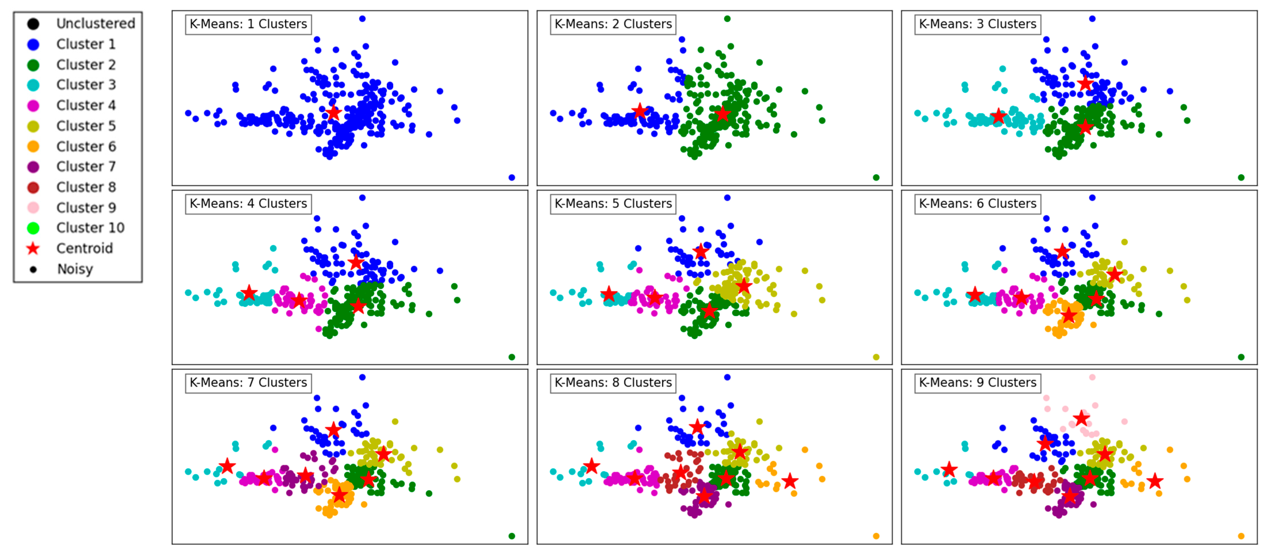
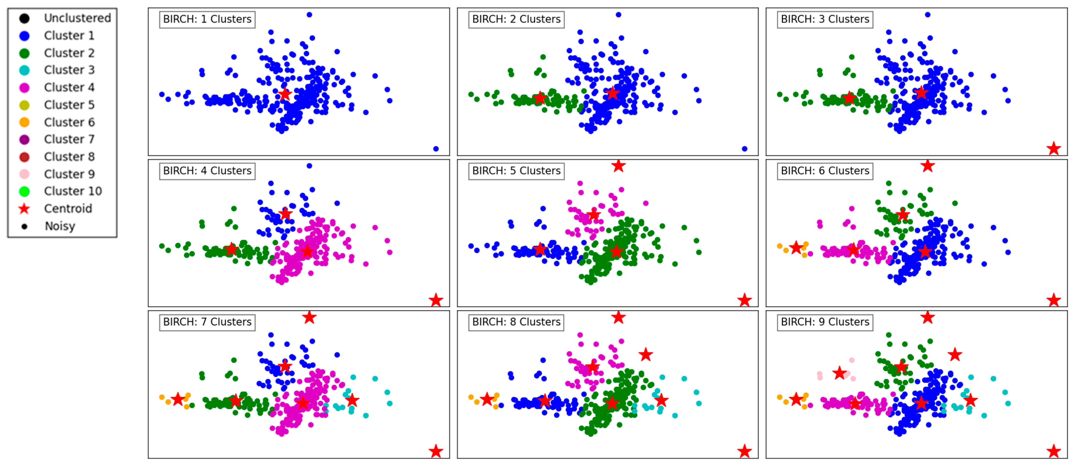

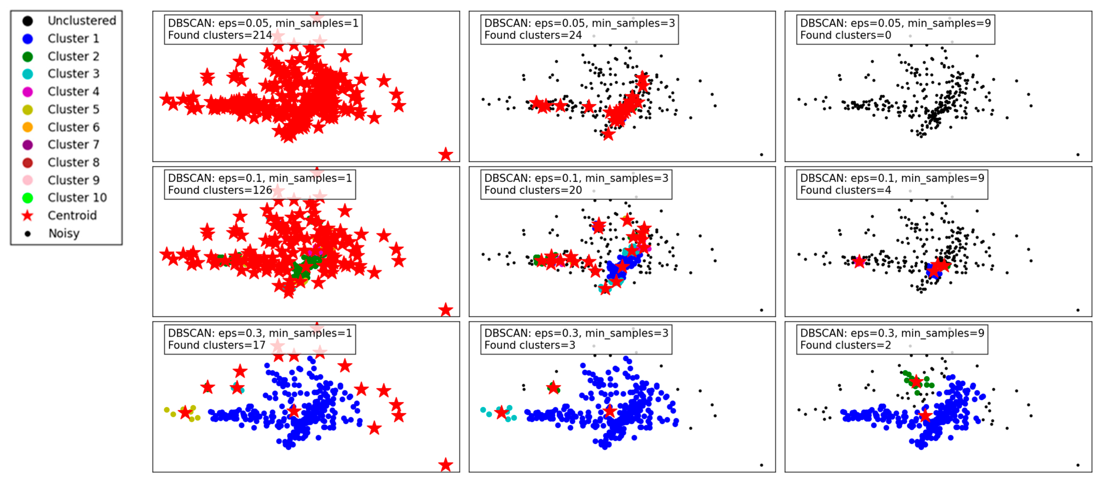
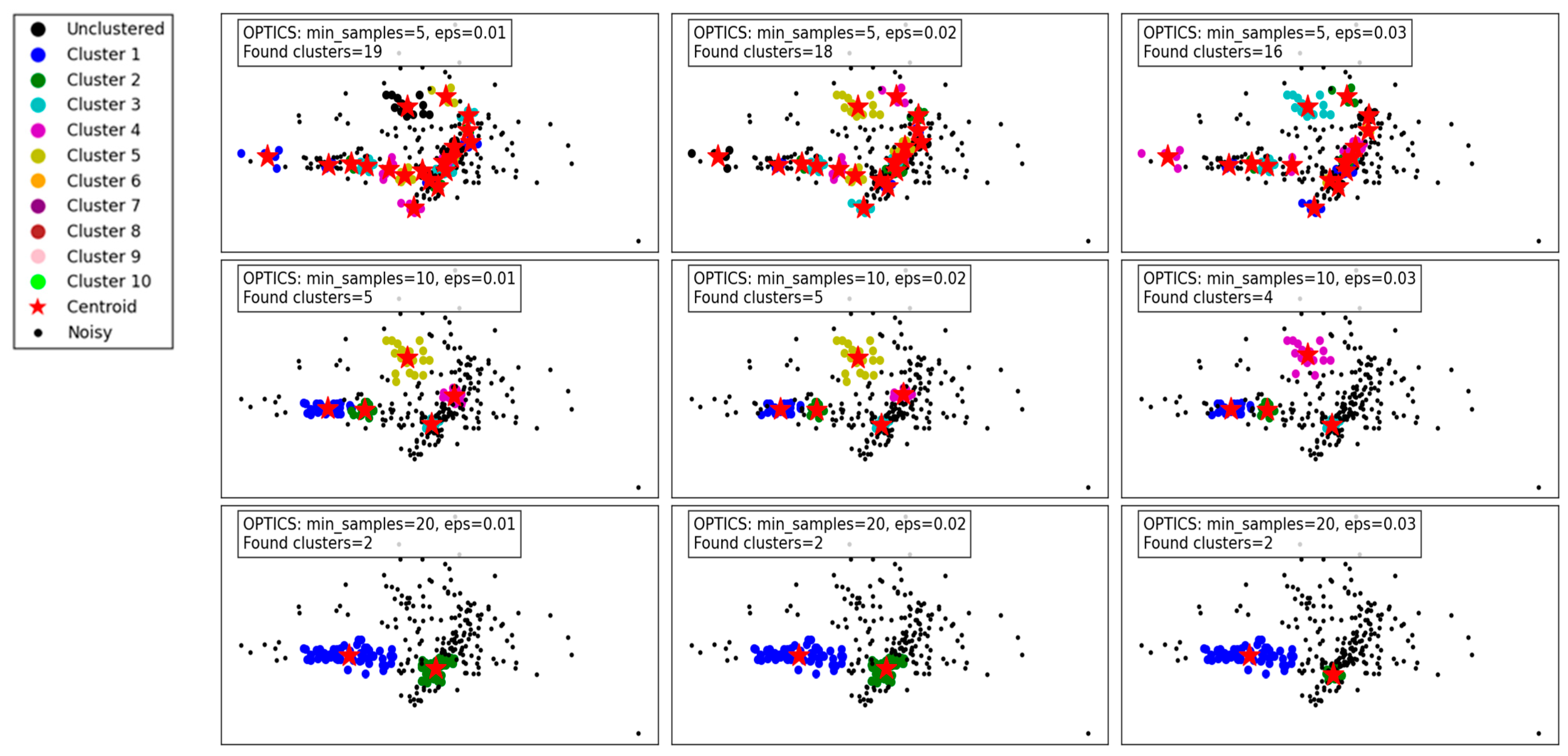

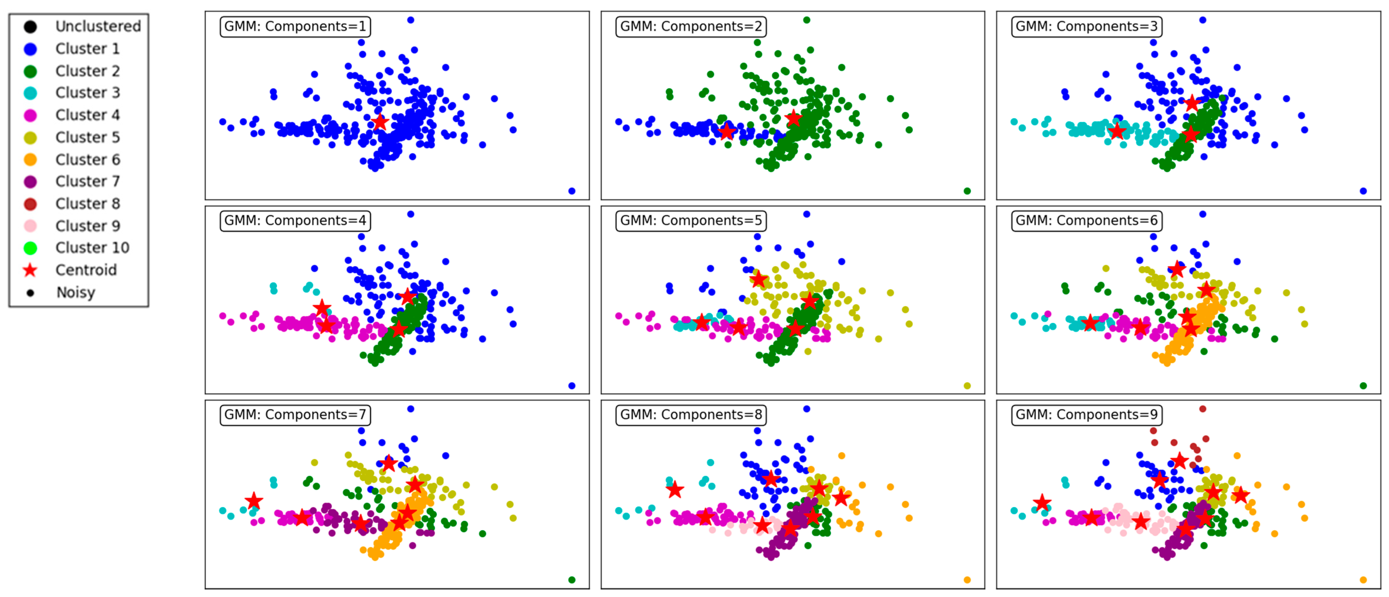
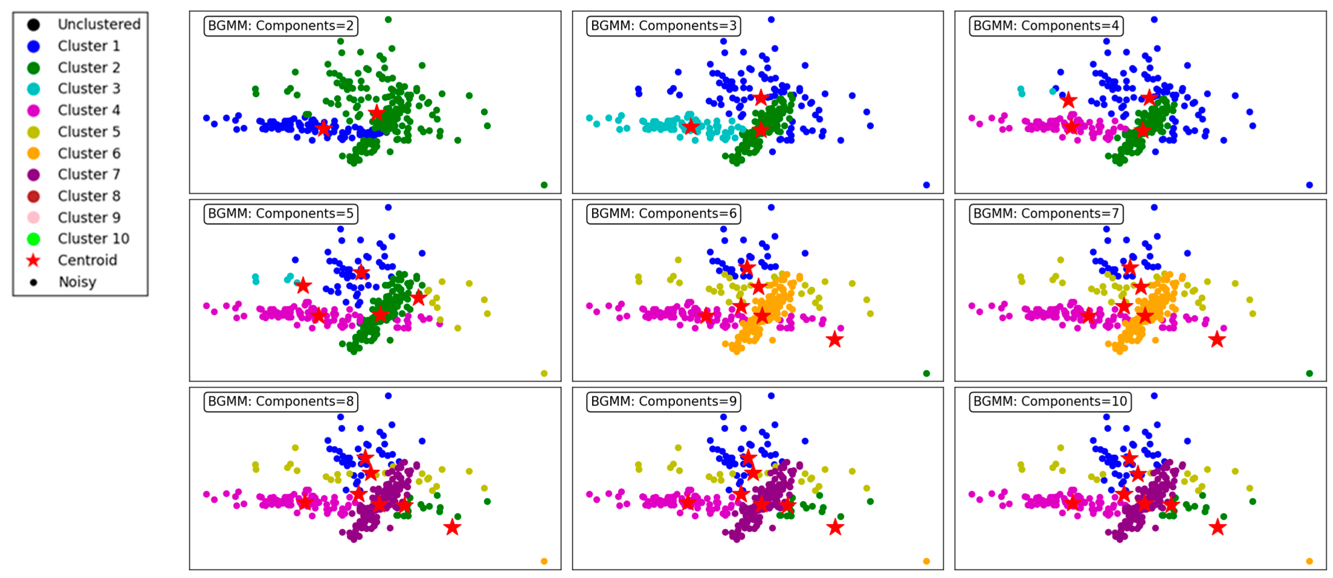

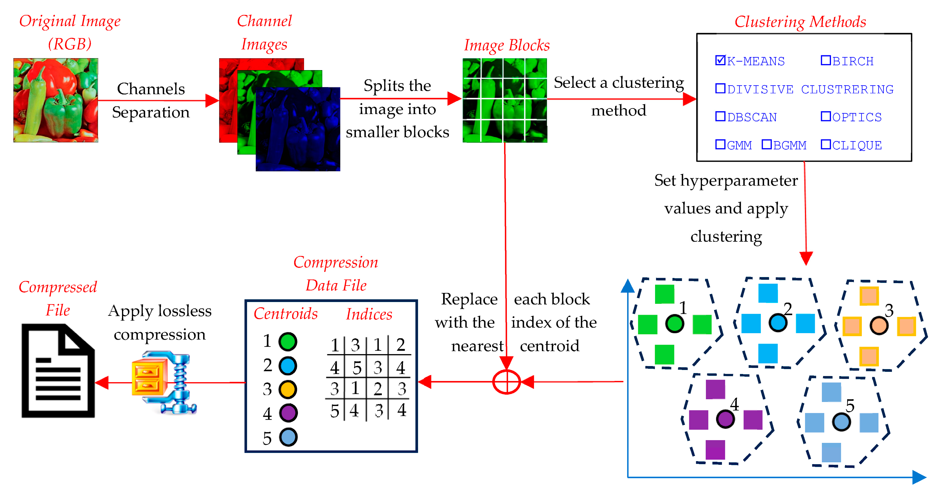
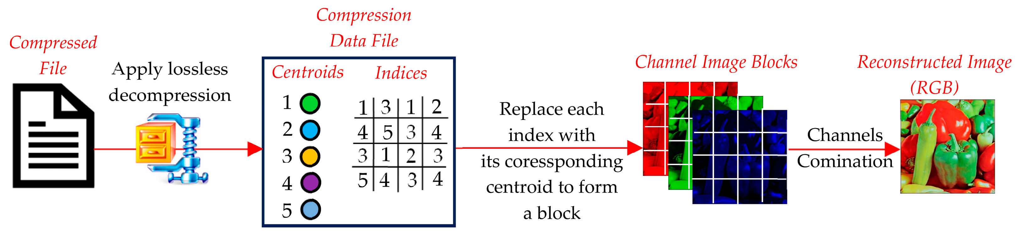

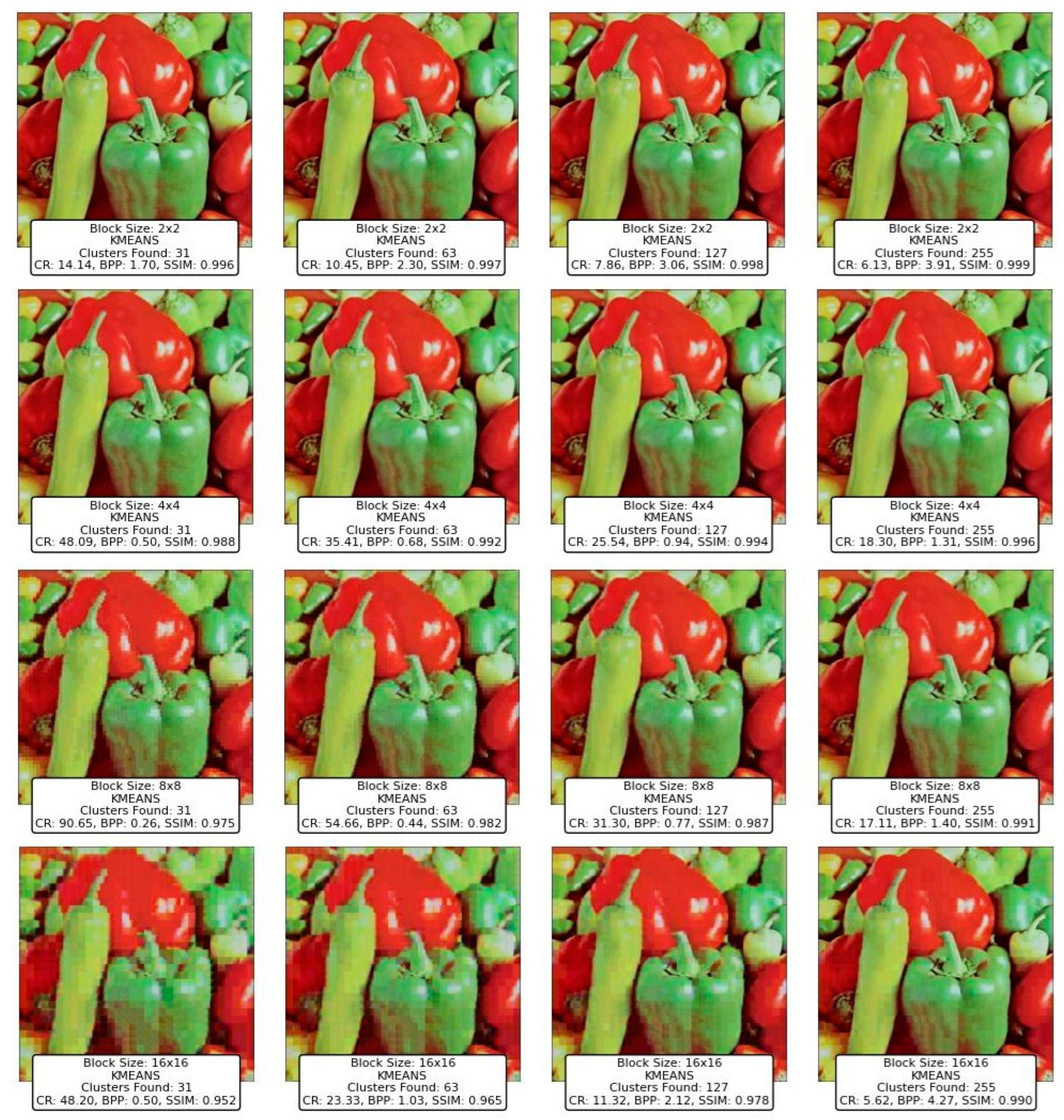

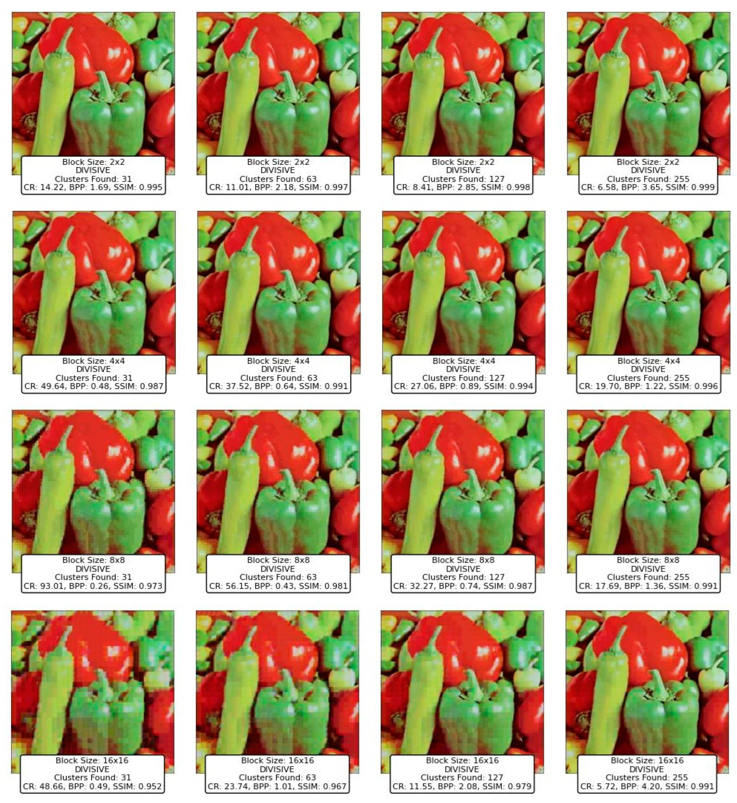
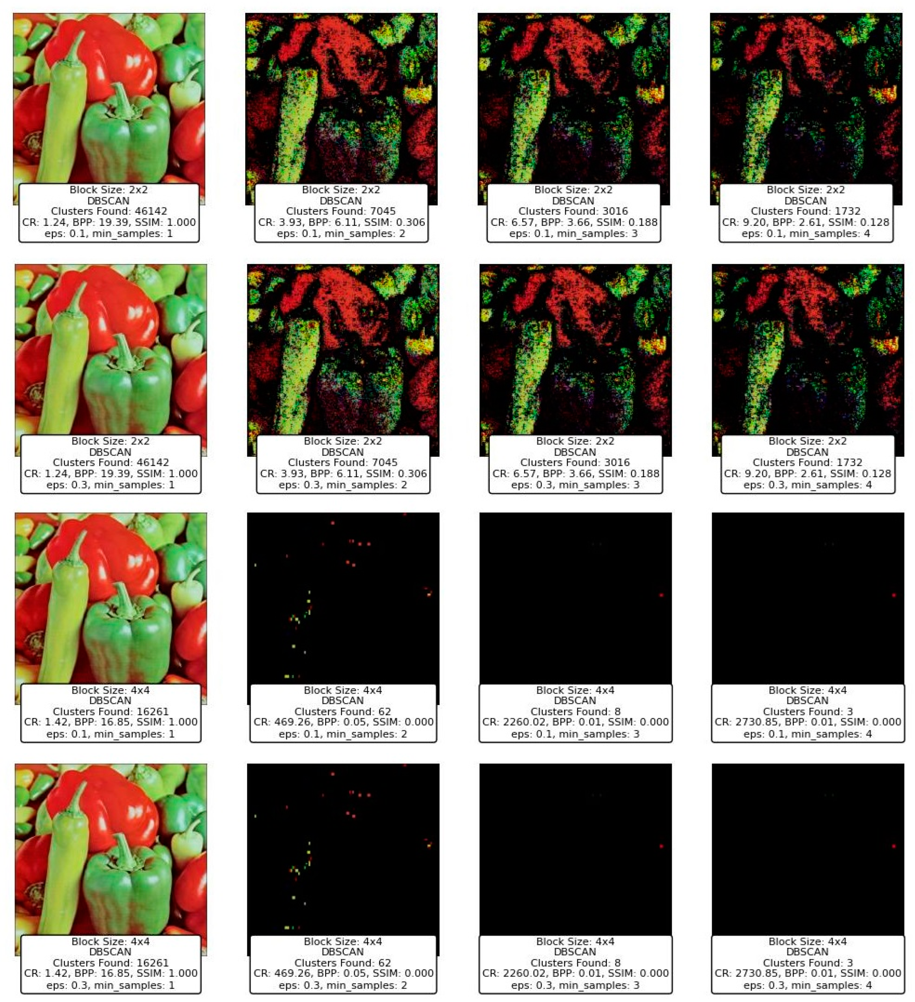
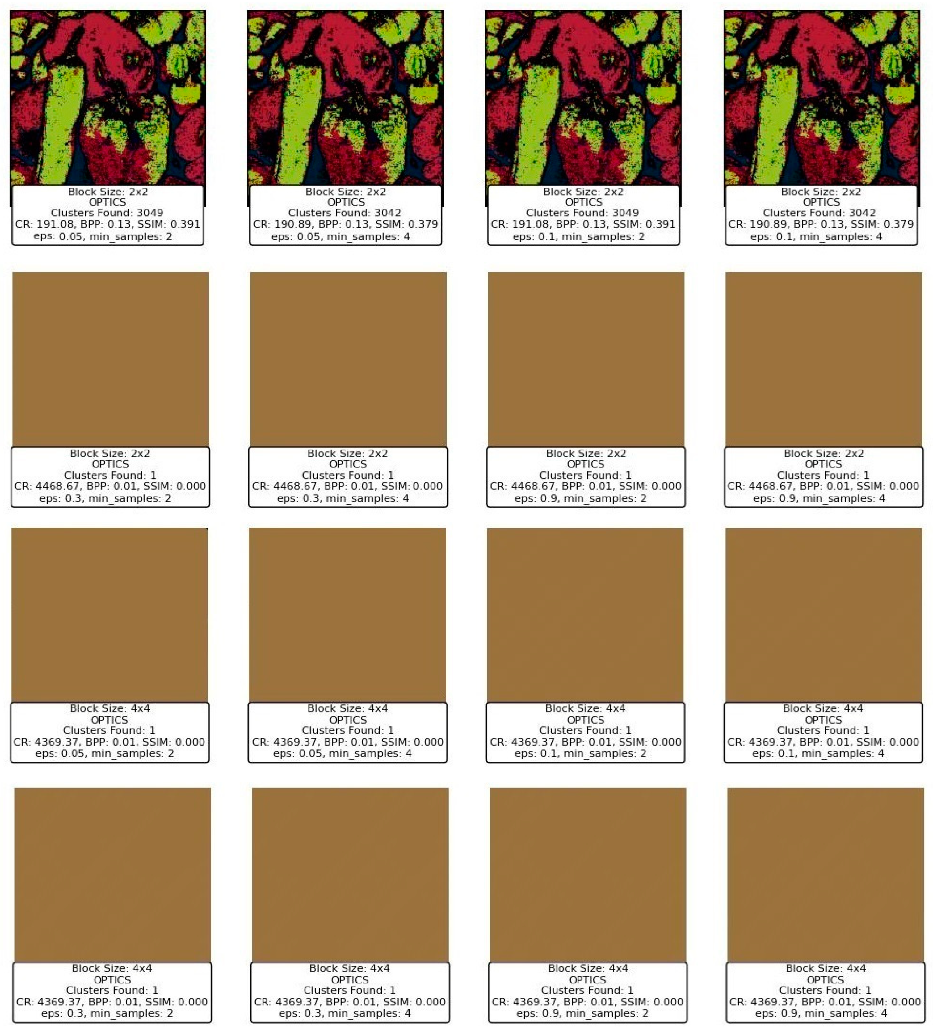
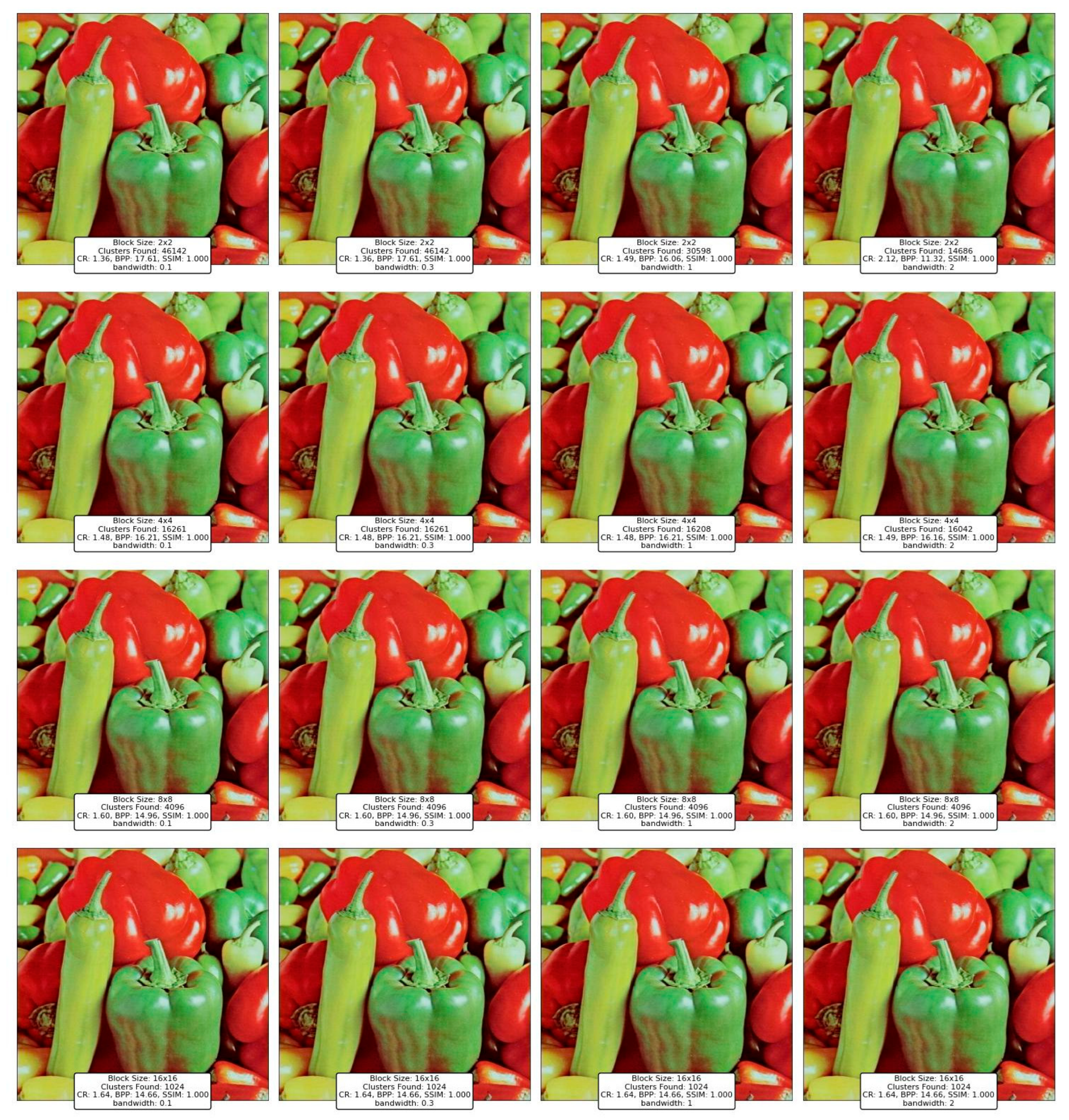
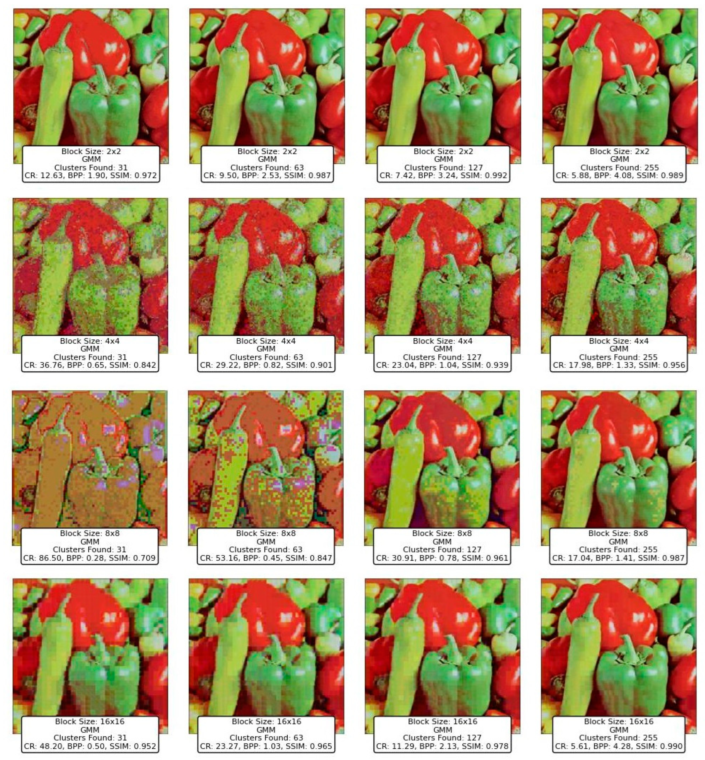

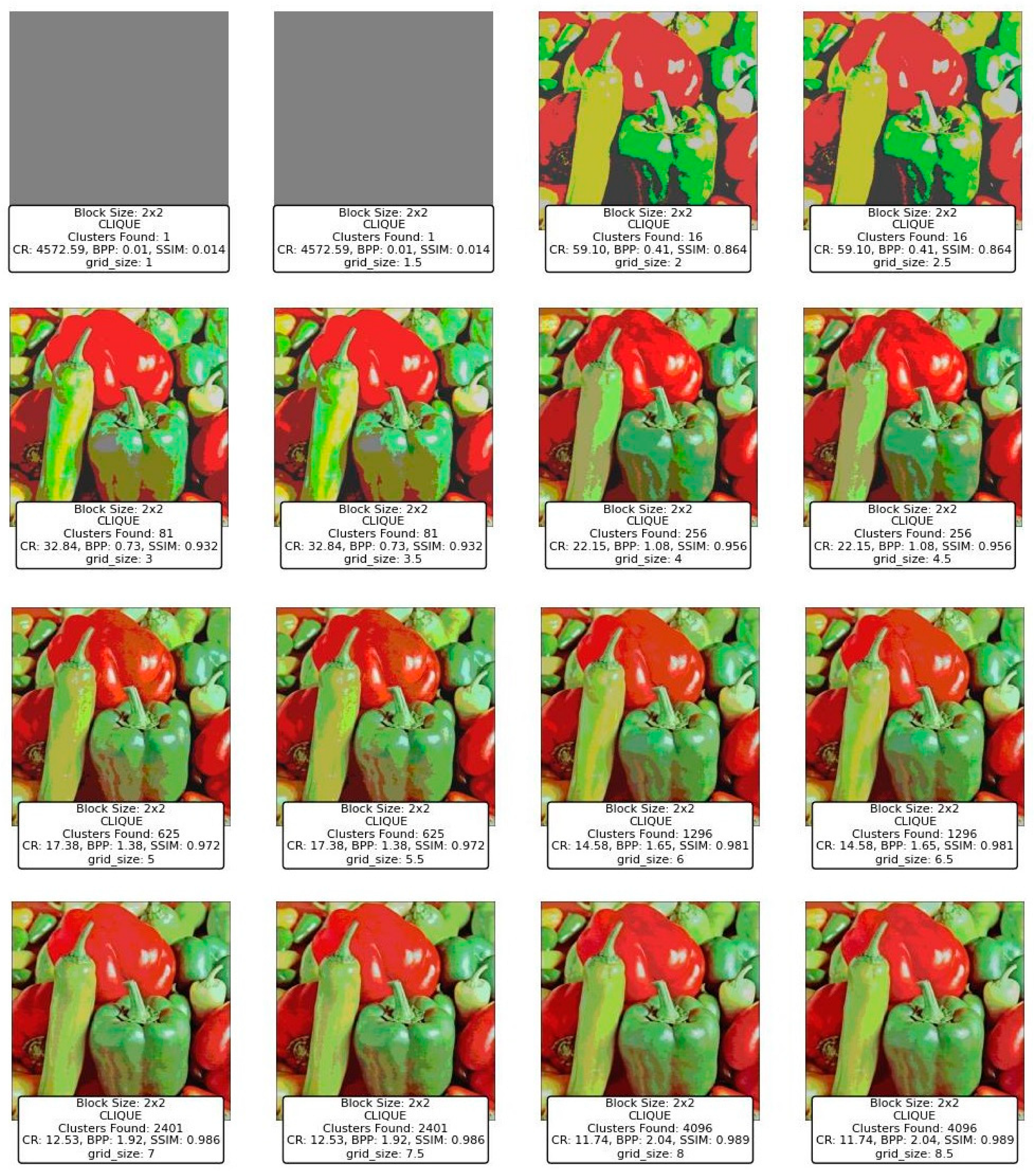

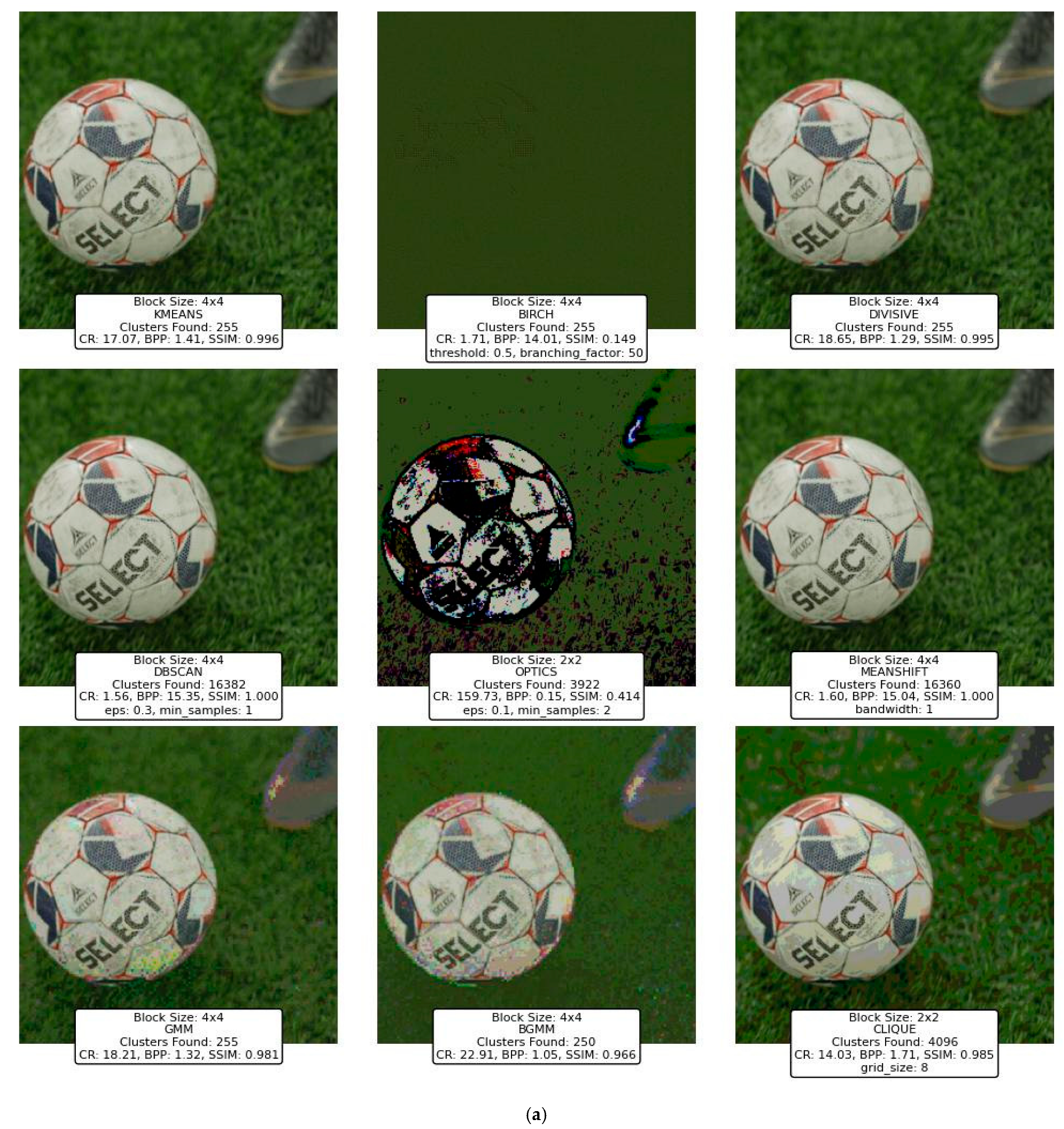
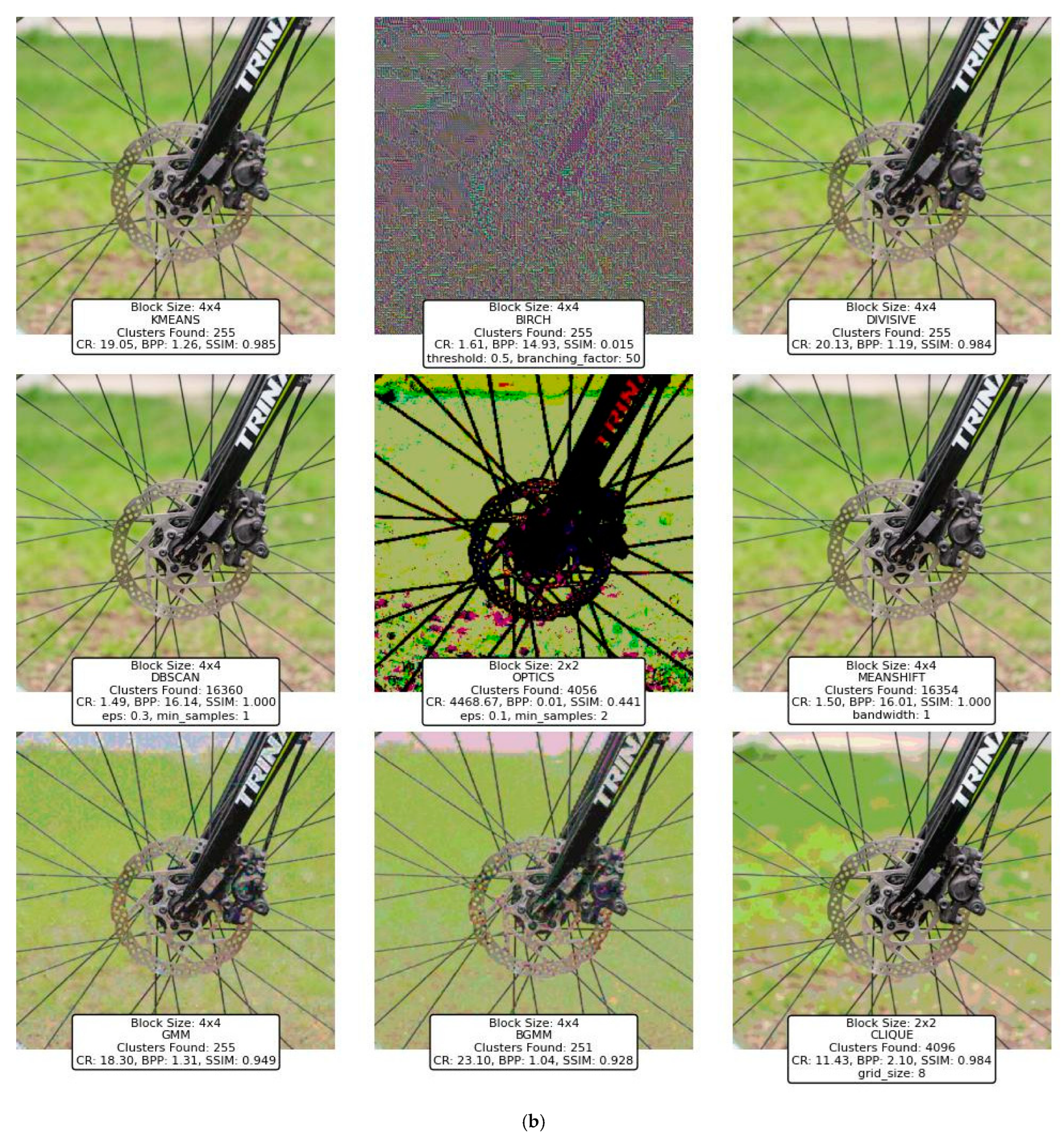
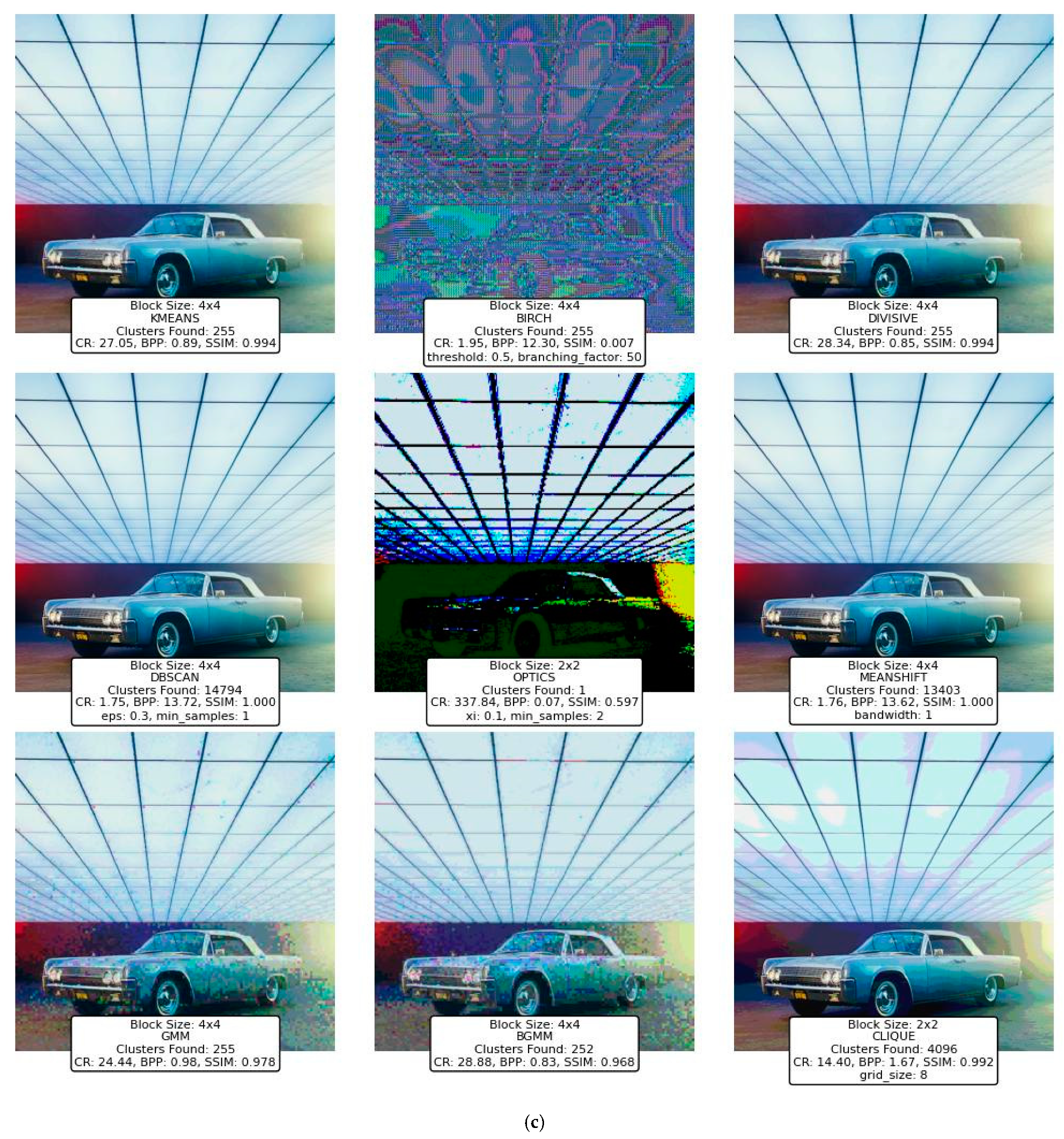
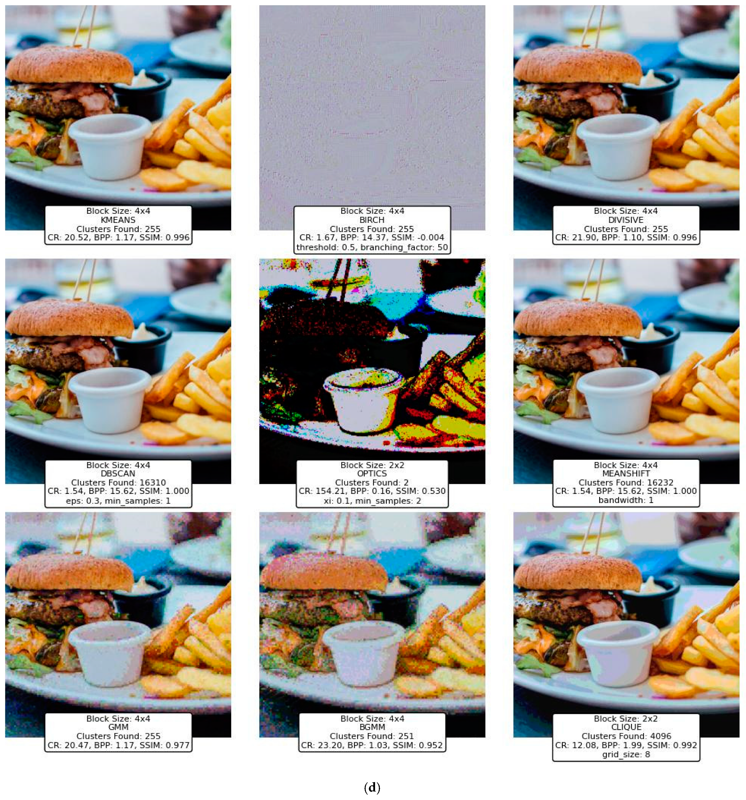
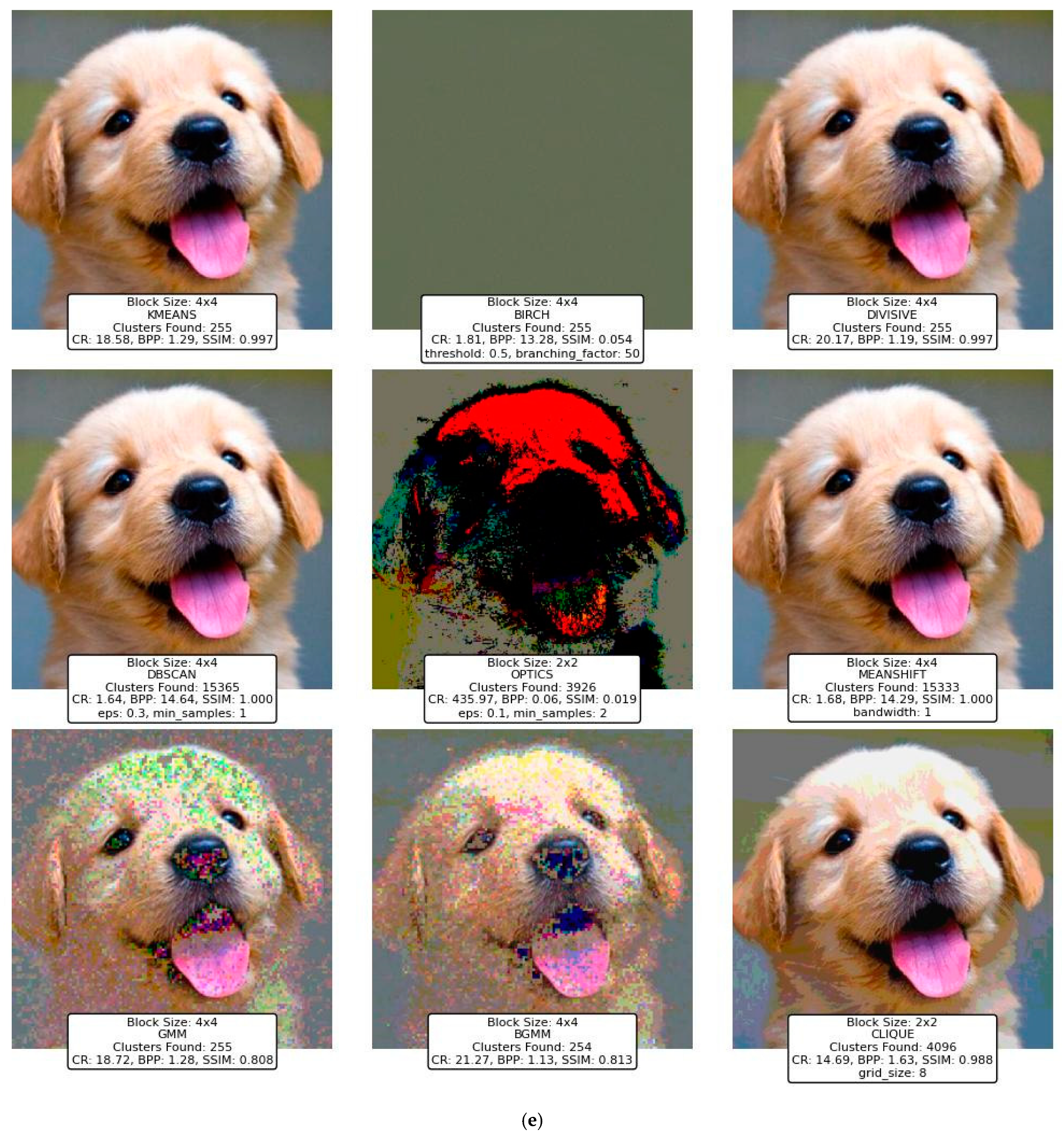


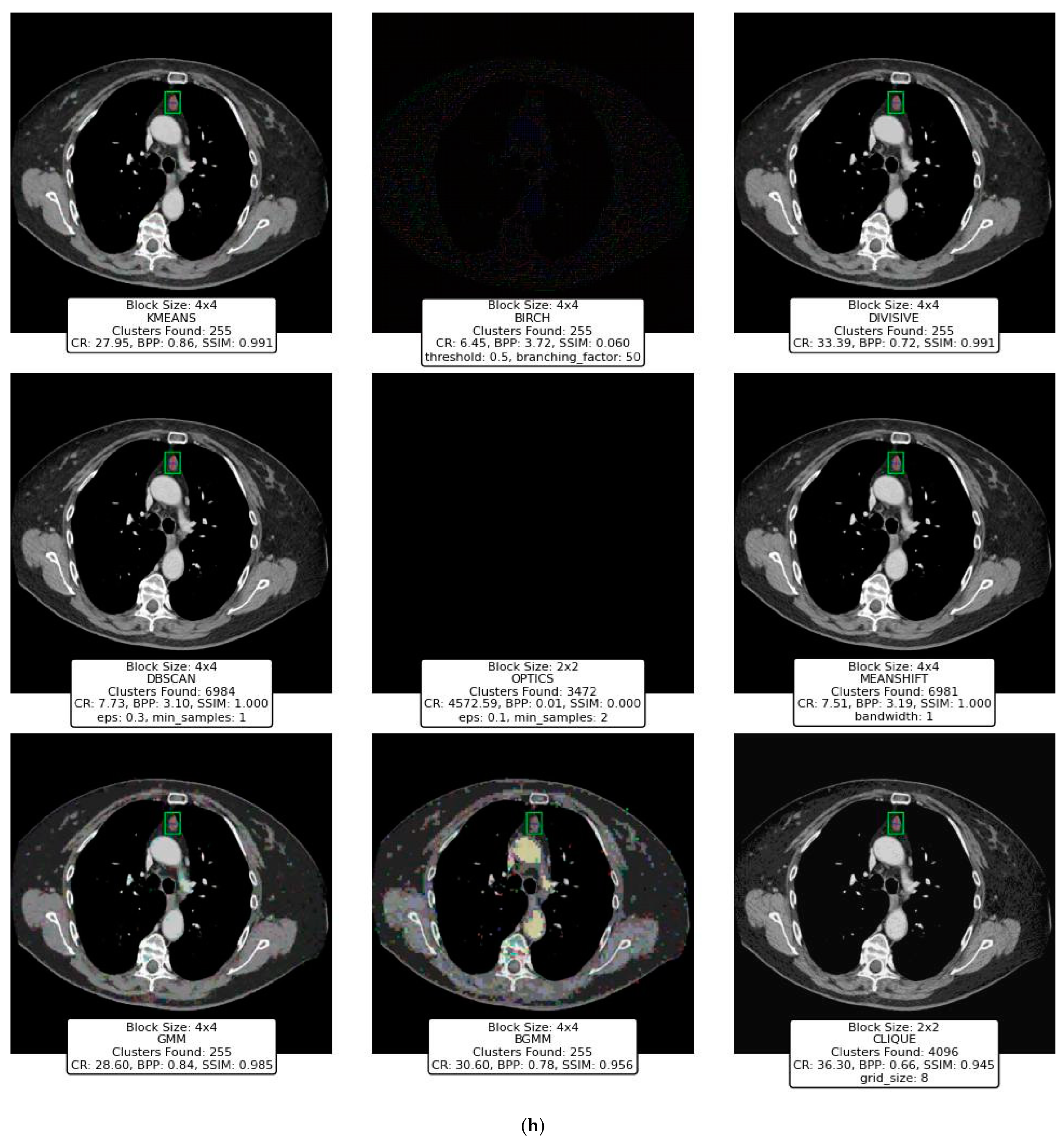


Disclaimer/Publisher’s Note: The statements, opinions and data contained in all publications are solely those of the individual author(s) and contributor(s) and not of MDPI and/or the editor(s). MDPI and/or the editor(s) disclaim responsibility for any injury to people or property resulting from any ideas, methods, instructions or products referred to in the content. |
© 2025 by the authors. Licensee MDPI, Basel, Switzerland. This article is an open access article distributed under the terms and conditions of the Creative Commons Attribution (CC BY) license (https://creativecommons.org/licenses/by/4.0/).