A Hardware-in-the-Loop Simulation Platform for a High-Speed Maglev Positioning and Speed Measurement System

Abstract

In order to solve the testing and verification problems at the early development stage of a high-speed Maglev positioning and speed measurement system (MPSS), a hardware-in-the-loop (HIL) simulation platform is presented, which includes induction loops, transmitting antennas, a power driver unit, a simulator based on a field-programmable gate array (FPGA), a host computer, etc. This HIL simulation platform simulates the operation of a high-speed Maglev train and generates the related loop-induced signals to test the performance of a real ground signal processing unit (GSPU). Furthermore, an absolute position detection method based on Gray-coded loops is proposed to identify which Gray-coded period the train is in. A relative position detection method based on height compensation is also proposed to calculate the exact position of the train in a Gray-coded period. The experimental results show that the positioning error is only 2.58 mm, and the speed error is 6.34 km/h even in the 600 km/h condition. The proposed HIL platform also effectively simulates the three kinds of operation modes of high-speed Maglev trains, which verifies the effectiveness and practicality of the HIL simulation strategy. This provides favorable conditions for the development and early validation of high-speed MPSS.

1. Introduction

As an innovative ground transportation system, Maglev trains use magnetic force to achieve contactless levitation, guidance, and propulsion, successfully overcoming the problems faced by conventional trains, such as wheel–rail adhesion limitations, mechanical noise, wear and tear, etc. [1,2]. They not only enrich existing modes of transport, reducing the speed gap between trains and planes, but also become a green mode of transport with their high efficiency and environmentally friendly features. With the continuous progress of technology, the 200–300 km/h medium- and low-speed Maglev trains have achieved commercial operation worldwide [3,4], while positioning and speed measurement engineering solutions have also tended to mature [5,6].

However, for the 600 km/h high-speed Maglev train, many technical challenges remain that are critical for safe and efficient operation [7,8]. At such high speeds, speed measurement and positioning have become increasingly difficult. Sensor accuracy and fast signal processing are critical, as even small errors can lead to significant positional deviations. In the field of traction control, the challenge is to provide precise power control to deliver considerable traction without compromising system stability. Vehicle-to-ground communication also faces obstacles, as maintaining ultra-reliable, low-latency data exchange becomes more demanding as speeds increase. Meanwhile, levitation control is heavily influenced by small fluctuations in the magnetic field and the air gap between the train and the track, necessitating the implementation of highly sensitive and adaptive control strategies. In particular, the speed measurement and positioning technology is not only the basis for the closed-loop control of the traction and operation control system of the high-speed Maglev train, but also the key to ensuring the safe and stable operation of the train [9]. Therefore, the speed measurement and positioning technology of the high-speed Maglev train is the focus of technological breakthroughs and technical application.

Because of the complexity of the operating environment of the Maglev train and the high construction cost, it is particularly important to construct an efficient and reliable test environment at the early stage of the MPSS [10]. The HIL semi-physical simulation technology provides an ideal solution for this purpose. It uses a real controller as the control unit, while the controlled object and the operating environment are presented in the form of a digital model, thus constructing a highly simulated HIL real-time simulation platform [11,12,13]. HIL simulation technology has been widely used in the transportation field [14,15,16]. Marinescu et al. [17] used HIL simulation to validate electric vehicle charging algorithms. Simulating scenarios under controlled conditions reduces the negative impact of smart body learning on the grid. However, the scalability of this approach in more complex network environments remains to be fully explored. Yang et al. [18] advanced the field by building a multiprocessor-based HIL platform designed for the real-time simulation of train faults within a traction control system (TCS). The downside is that the integration of multiprocessor architectures may lead to increased system complexity and maintenance challenges. Zhao et al. [19] utilized an HIL test system to validate the control strategy of a semi-active suspension system. The results confirmed the feasibility of HIL for performance evaluation, but the research did not address in depth the potential limitations of sensor accuracy under high electromagnetic interference (EMI) conditions. Bernal et al. [20] applied the HIL technology to test a novel node architecture for wheel plane detection sensors. The feasibility of the sensor design was successfully explored without interfering with real-world operation, although further field validation is required to assess long-term reliability under different operating conditions.

The earliest applications of HIL simulation in Maglev systems focused on the verification and optimization of control systems. In the late 1980s, the German Transrapid project [21] pioneered the development of automated procedures for the analysis and design of nonlinear control systems. While this approach was innovative at the time, it encountered challenges in adapting to the rapidly evolving control requirements of modern Maglev systems. Subsequent studies have further refined the application of HIL in this area. Wang et al. [22] verified the effectiveness and feasibility of a velocity estimation scheme for vector-controlled linear induction motor (LIM) drives, especially for low- and medium-speed Maglev applications. Similarly, Hu et al. [23] applied HIL simulation to evaluate LIM control algorithms, thus providing valuable reference data for traction control. However, both of these studies addressed LIM applied to Maglev trains without focusing on the actual operation of the trains. Jandaghi et al. [24] introduced a real-time digital simulation drive system based on FPGA technology for Maglev applications. Their FPGA-based approach improves simulation accuracy and real-time performance, despite higher initial development complexity and cost. In addition, HIL technology has been extended to other key components of Maglev systems, including operation control systems (OCS) [25,26], vehicle stability control [27,28], and TCS [29,30].

However, the application of the above HIL simulation technology is aimed at the operation control of the Maglev train or the verification of the system function, and there is a lack of simulation platforms for the MPSS, especially for the high-speed trains over 600 km/h. Compared with traditional hardware-based testing solutions, HIL simulation does not require on-site testing or the construction of a complete physical system. By building a highly simulated real-time test platform, it greatly reduces the cost of testing and makes testing more targeted. In order to more intuitively show the innovative aspects of the HIL simulation platform proposed in this paper, several typical test solutions in the field of Maglev trains are compared with it.

Table 1. Comparative analysis of the proposed HIL simulation platform and existing solutions.

Solution	Test Object	Cost	Complexity	Ease of Implementation	Accuracy	Flexibility
Traditional Hardware-based 1	Actual requirements	high	high	low	low	low
Existing HIL-based 2	LIM	low	high	low	high	low
	OCS	moderate	high	moderate	moderate	low
	TCS	moderate	low	low	high	low
Proposed HIL Platform	MPSS	low	low	high	high	high

¹ The traditional hardware-based testing solution performs testing on complete systems based on actual requirements. However, it has the disadvantages of high cost and complexity. Accuracy and flexibility cannot be guaranteed. ² HIL-based test solutions mentioned in references [22,23,24,25,26,28,29] are included. These solutions target different test objects.

shows the advantages of the proposed HIL platform in terms of cost, complexity, and ease of implementation. In fact, there is no simulation test platform reported for MPSS. The HIL simulation platform proposed in this paper provides an effective solution for it. By simplifying the system integration and modular design approach, the system has lower complexity and is easier to implement. Subsequent experiments show that the platform can simulate multiple train operation modes with better performance in terms of flexibility and accuracy.

In this paper, an HIL simulation platform on the high-speed Maglev positioning and speed measurement is reported to solve the related testing problems. Firstly, an absolute position detection method based on Gray-coded loops and a relative position detection method based on height compensation are proposed. The experimental results show that they effectively eliminate the cumulative error of positioning data during the operation of the Maglev train, relative to the traditional rail transit positioning methods. Secondly, the generation methods of some key simulation signals, such as loop-inducted signals and antenna pulse width modulation (PWM) signals in MPSS, are deeply analyzed. On this basis, the HIL simulation platform was built for testing the GSPU, which is the core of MPSS. The HIL simulation platform includes induction loops, transmitting antennas, a power driver unit, an FPGA simulator, and a host computer. This platform not only maximally simulates the operating environment but also significantly reduces the cost and risk of on-site debugging. It provides strong experimental support for the development of MPSS and lays a solid foundation for subsequent system optimization.

2. Principle of Positioning

During the operation of the Maglev train, the vehicle magnetic field interacts with the track magnetic field to generate a horizontal thrust that pushes the train forward [31,32]. To ensure that the train’s magnetic field is synchronized with the track’s magnetic field and that the current frequency of the electromagnets on the track matches the train’s operating speed, the traction system must acquire real-time and accurate information about the train’s position [33,34]. Therefore, the MPSS plays a decisive role in the safe and efficient operation of magnetic levitation trains.

2.1. Composition and Principle of MPSS

In this paper, the MPSS is based on Gray-coded loops. The main reason for using Gray-coded loops is their unique error-reducing properties: since neighboring codes differ by only one bit, the risk of misinterpretation during signal conversion is greatly reduced. This is particularly beneficial in high-speed applications, such as in 600 km/h Maglev trains, where fast movements and environmental disturbances can easily lead to errors. In addition, the use of Gray-coded loops allows for the development of ground-based positioning and speed measurement, which greatly reduces the system’s dependence on vehicle-to-ground communications. This not only enhances the measurement system’s ability to withstand external interference but also helps achieve millimeter-level positioning accuracy. By utilizing these advantages, the method improves the accuracy, continuity, and real-time performance of the system, making it a cost-effective and reliable solution for high-speed Maglev train operations.

The MPSS consists of three parts: a vehicle transmission unit (VTU), an induction loop unit (ILU), and a GSPU. In the VTU, the PWM signal generated by the controller is amplified by the driver and injected into the transmitting antenna. An alternating magnetic field is generated around it, and a voltage signal with the same frequency as the current frequency of the transmitting antenna is induced in the ILU. The induced signals are transmitted to the GSPU after the integration of the start box and the terminal box, and the GSPU gets the position and speed information of the train. Therefore, the core of the MPSS is the GSPU, which is also the test object of the HIL simulation platform in this paper. The platform simulates a realistic operating environment by reconstructing induced signals and PWM signals. The structure of the MPSS is shown in Figure 1.

The MPSS divides the positioning process of a Maglev train into two stages: absolute position detection and relative position detection. The absolute position detection locates the train by positioning it within a Gray-coded period, while relative position detection further locates the train’s precise position within that Gray-coded period. The combination of the two achieves the precise positioning of the Maglev train. The speed of the train is then obtained by calculating the ratio of the distance Δd between two adjacent crossings to the elapsed time Δt:

$$\mathrm{V}=\Delta \mathrm{d}/\Delta \mathrm{t}.$$

(1)

2.2. Absolute Position Detection Based on Gray-Coded Loops

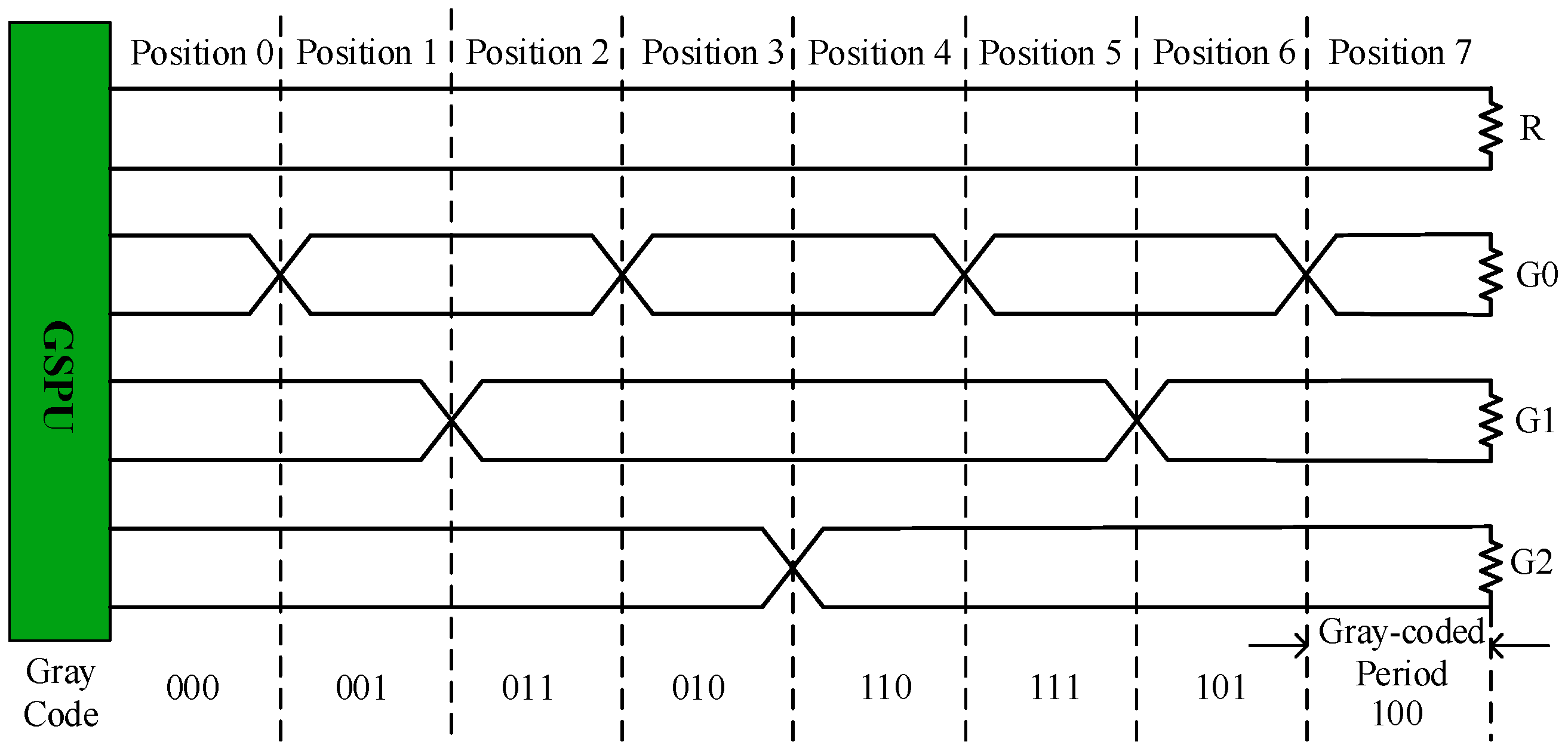
In the MPSS, a group of reference loops R and several groups of address loops Gn arranged according to the Gray code law are laid directly under the transmitting antenna of the train. The address loops cross once every certain step, while the reference loops do not cross into the ILU. The number of address loops should be set according to the actual engineering requirements [35], too many will lead to the problem of induction signal attenuation, too few will lead to the GSPU setting distance being too close, and will increase the cost.

In this paper, we set up six groups of address loops, named G0~G5. Since there are $2^6=64$ codes for the six address loops, due to space constraints, a simplified explanation of its working principles with the three groups of address loops is shown in Figure 2.

When an alternating current is injected into the transmitting antenna, an alternating electromagnetic field is created around it. The address loops are approximately located in a uniformly distributed magnetic field [36]. Each loop generates a corresponding induced signal, which is sent to the GSPU. Since the reference loop is not crossed, its induced signal does not change with the position of the antenna. Instead, whenever the transmitting antenna passes through the cross node of the address loops, the phase of the induced signal changes by 180°. The voltage signals in the address loops are compared with the voltage signal in the reference loop; if the two are in the same phase, it represents code ‘0’; if the two are in opposite phase, it represents code ‘1’.

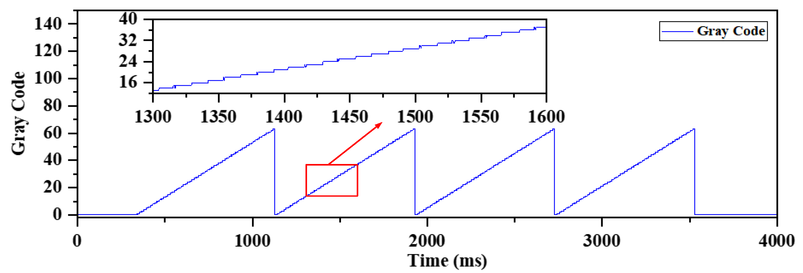
When the antenna is in position 0, the address loops G0, G1, and G2 have not passed through the cross node, and the phase of the induced signals is the same as that in reference loop R. The Gray code for this position is ‘000’. When the antenna moves from position 0 to position 7, only one of the induced signals of the address loops is inverted. The corresponding Gray code also changes by only one bit, and the distance represented by one Gray code is a Gray-coded period. After decoding the Gray code to get the corresponding natural decimal number, the position of the train can be positioned within a Gray-coded period, thus completing the absolute positioning of the train.

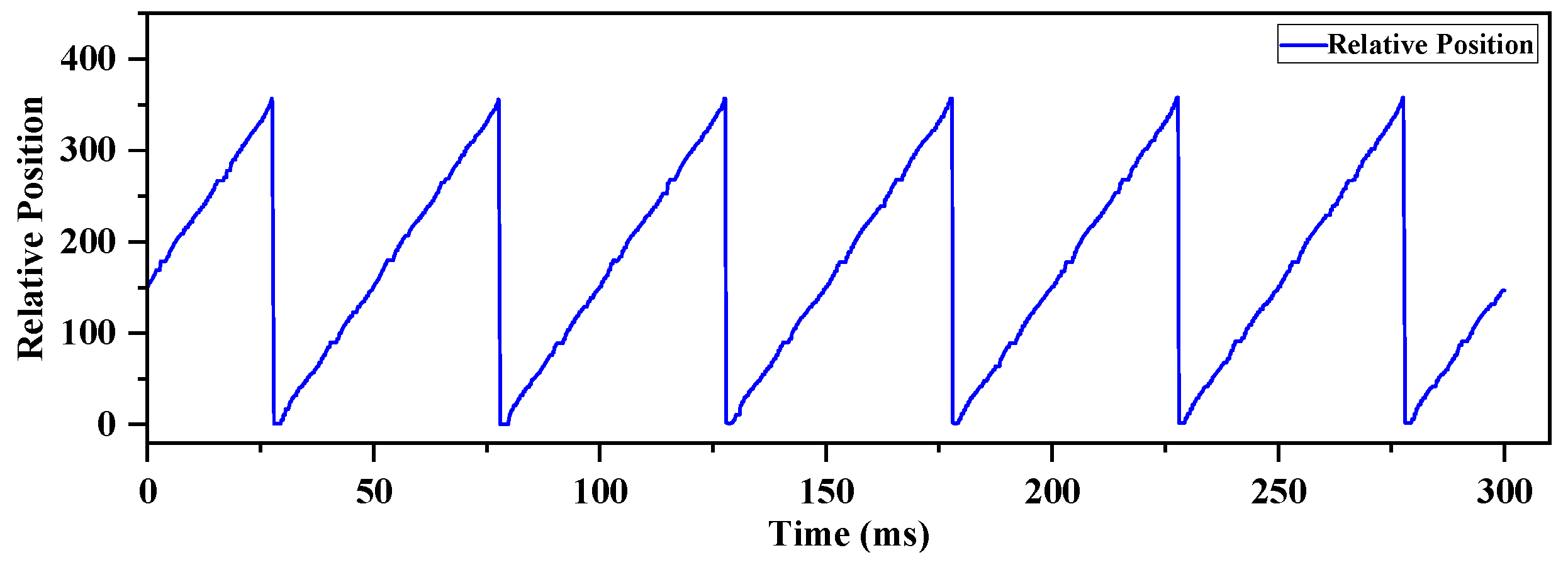
2.3. Relative Position Detection Based on Height Compensation

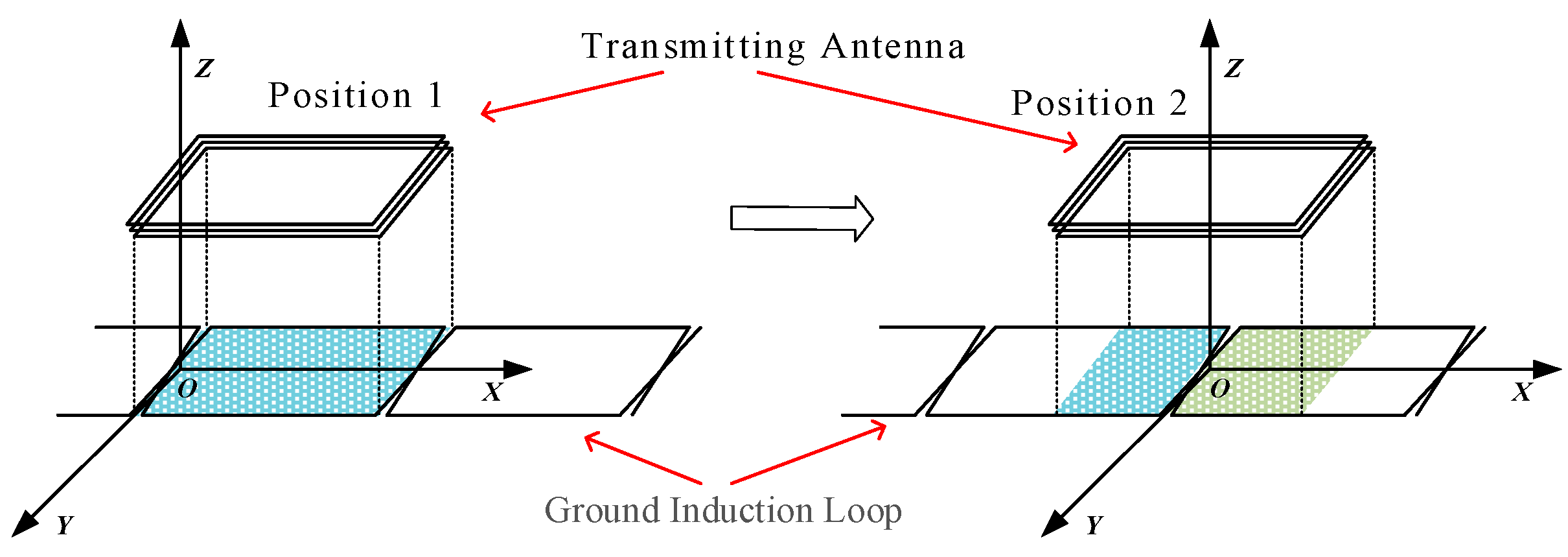
The relative position is detected based on the cyclic change of the induction signal, the principle of which is shown in Figure 3, in which the ground induction loop is the lowest address loop G0. When the transmitting antenna moves to position 1, the effective induction area of the loop is the largest, and the magnetic flux that crosses the loop is the largest, so the amplitude of the induction signal is also the largest. When the transmitting antenna moves to position 2, the magnetic fluxes on both sides of the cross node are approximately equal, and the overall magnetic flux of the loop is approximately zero, so the amplitude of the induction signal is also close to zero. When in the process of moving from position 1 to position 2, it means that the relative position of the transmitting antenna within a Gray-coded period can be exactly calculated according to the real amplitude of the induced signal.

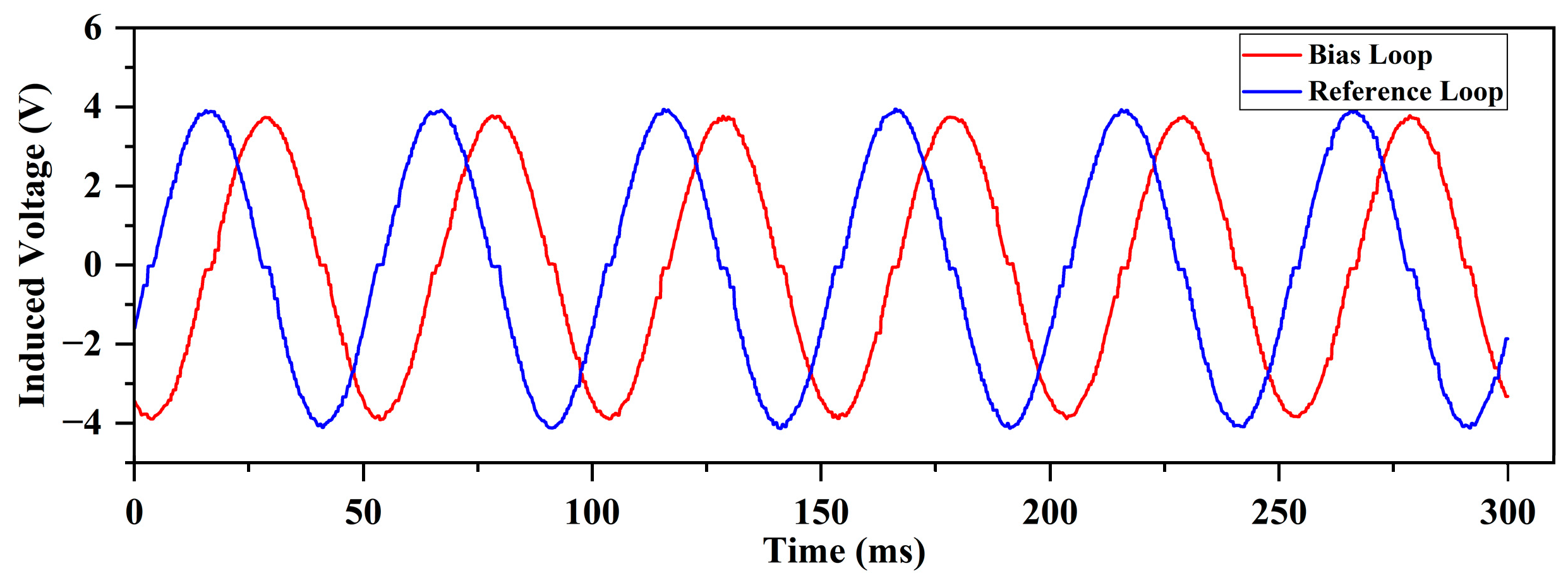
However, the distance between the transmitting antenna and the sensing loop changes as the train travels on the track [37], and the amplitude of the induced signal changes. This leads to an error in the inverse deduction of the relative position from the induced signal amplitude. To solve this problem, the bias loop SG0 for relative positioning is laid out in this paper, which has the same structure and crossing cycle as the lowest address loop G0, but the loop cross node differs by half a crossing cycle, and the laying method of G0 and SG0 and their induced signal variations are shown in Figure 4.

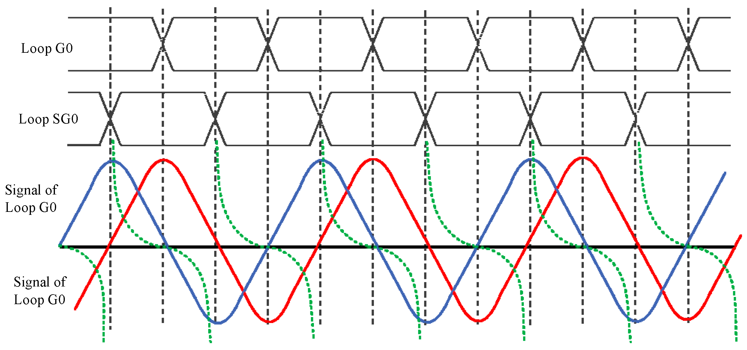
In Figure 4, the phase ahead of the curve is the demodulated envelope of the G0-induced signal, and the phase-lag curve is the demodulated envelope of the SG0-induced signal, and the phase difference of the signals between them is 90 degrees, which can be expressed, respectively, as follows:

$$\mathrm{U}\left(\mathrm{G}0\right)=\mathrm{f}\left(\mathrm{h}\right)\mathrm{g}\left(\mathrm{s}\right)$$

(2)

$$\mathrm{U}(\mathrm{S}\mathrm{G}0)=\mathrm{f}(\mathrm{h})\mathrm{g}(\mathrm{s}-{\displaystyle \frac{1}{2}}\mathrm{l}),$$

(3)

where g(s) is the envelope signal at the standard height; f(h) is a function related to the suspension height h, which is linear in the range of the suspension fluctuation; s is the distance between the antenna and the starting point of the ILU; and l is the Gray-coded period. To overcome the positioning error caused by the height fluctuation, the ratio of the amplitudes in the G0 and SG0 loops is calculated as follows:

$${\displaystyle \frac{\mathrm{U}(\mathrm{G}0)}{\mathrm{U}(\mathrm{S}\mathrm{G}0)}}={\displaystyle \frac{\mathrm{g}(\mathrm{s})}{\mathrm{g}(\mathrm{s}-\frac{1}{2}\mathrm{l})}}.$$

(4)

In Equation (4), the ratio depends entirely on the position of the train. It means that the influence of the train height fluctuation on the positioning accuracy is eliminated. In the actual operation, a complete mapping table of the ratios and relative position information was created, and the accurate relative position information can be easily obtained by indexing this table.

3. Signal Reconstruction Based on Parallel Signal Simulation

To simulate the real operating environment of the GSPU, it is necessary to reconstruct some key signals, including the inductive signals of the loops and the PWM signals injected into the transmitting antenna, etc. The HIL simulation platform is set up with eight groups of induction loops, which include a group of reference loops, six groups of address loops used for absolute position detection, and a group of bias loops used for relative position detection. In actual operation, these eight groups of induction loops receive signals with different amplitudes and phases.

Based on this, the simulation platform adopts a strategy of parallel signal simulation and sets up a separate transmitting antenna for each pair of induction loops. When simulating train operation, the current parameters of each transmitting antenna are adjusted independently according to the real-time position of the train. This results in the simulation of the signals of the loops during train operation. Therefore, the relationship between the amplitude of the induction signal of the loop line and the train running position is analyzed in the following, and the control strategy of the PWM signal parameters of the transmitting antenna is determined.

3.1. Analysis of Induced Signal Amplitude and Train Position

Based on the principle of the positioning and speed measurement of the induction loop, each position of the transmitting antenna corresponds to a unique induced signal amplitude. Therefore, to dynamically adjust the current magnitude of each transmitting antenna according to the simulated position of the train, a mathematical model describing the relationship between the induced signal amplitude of the loop and the position of the transmitting antenna is required.

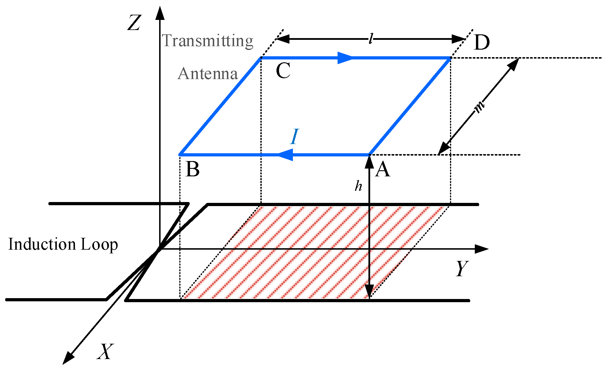
In practice, since the reference loop is not crossed, its induced signal amplitude remains constant during antenna movement, and thus only a fixed current needs to be injected into the corresponding transmitting antenna. As for the address loops and the bias loop, they can be grouped into the same category for discussion. Further, taking the lowest address loop G0 as an example, Figure 5 shows the positional relationship between the transmitting antenna and the address loop.

Both are of equal width, and the transmitting antenna is wound by a multi-turn coil in a rectangular shape. Considering that the strength of the magnetic field outside the closed coil decays rapidly and the transmitting antenna is close to the induction loop, the effective area of the magnetic field across the induction loop can be approximated as the projection of the transmitting antenna in the loop. Consider that the transmitting antenna is a single-turn coil consisting of segments AB, BC, CD, and DA. The magnetic induction at any point P(x,y) consists of the superposition of the magnetic fields produced by these four electrified wires. The expression for the magnetic induction at point P was obtained as follows:

$${\overline{\mathrm{B}}}_{\mathrm{A}\mathrm{B}}={\displaystyle \frac{{\mathsf{\mu }}_0\mathrm{I}}{4\mathsf{\pi }{\mathsf{\rho }}_1}}\left[{\displaystyle \frac{\mathrm{l}/2+\mathrm{y}}{\sqrt{{\mathsf{\rho }}_1^2+(\mathrm{I}/2+\mathrm{y}{)}^2}}}+{\displaystyle \frac{\mathrm{l}/2-\mathrm{y}}{\sqrt{{\mathsf{\rho }}_1^2+(\mathrm{I}/2-\mathrm{y}{)}^2}}}\right]{\overrightarrow{\mathrm{e}}}_{\mathsf{\Phi }1}$$

(5)

$${\overrightarrow{\mathrm{B}}}_{\mathrm{B}\mathrm{C}}={\displaystyle \frac{{\mathsf{\mu }}_0\mathrm{I}}{4\mathsf{\pi }{\mathsf{\rho }}_2}}\left[{\displaystyle \frac{\mathrm{m}/2+\mathrm{x}}{\sqrt{{\mathsf{\rho }}_2^2+(\mathrm{m}/2+\mathrm{x}{)}^2}}}+{\displaystyle \frac{\mathrm{m}/2-\mathrm{x}}{\sqrt{{\mathsf{\rho }}_2^2+(\mathrm{m}/2-\mathrm{x}{)}^2}}}\right]{\overline{\mathrm{e}}}_{\mathsf{\Phi }2}$$

(6)

$${\overrightarrow{\mathrm{B}}}_{\mathrm{C}\mathrm{D}}={\displaystyle \frac{{\mathsf{\mu }}_0\mathrm{I}}{4\mathsf{\pi }{\mathsf{\rho }}_3}}\left[{\displaystyle \frac{\mathrm{l}/2-\mathrm{y}}{\sqrt{{\mathsf{\rho }}_3^2+(\mathrm{l}/2-\mathrm{y}{)}^2}}}+{\displaystyle \frac{\mathrm{l}/2+\mathrm{y}}{\sqrt{{\mathsf{\rho }}_3^2+(\mathrm{l}/2+\mathrm{y}{)}^2}}}\right]{\overline{\mathrm{e}}}_{\mathsf{\Phi }3}$$

(7)

$${\overrightarrow{\mathrm{B}}}_{\mathrm{D}\mathrm{A}}={\displaystyle \frac{{\mathsf{\mu }}_0\mathrm{I}}{4\mathsf{\pi }{\mathsf{\rho }}_4}}\left[{\displaystyle \frac{\mathrm{m}/2-\mathrm{x}}{\sqrt{{\mathsf{\rho }}_4^2+(\mathrm{m}/2-\mathrm{x}{)}^2}}}+{\displaystyle \frac{\mathrm{m}/2+\mathrm{x}}{\sqrt{{\mathsf{\rho }}_4^2+(\mathrm{m}/2+\mathrm{x}{)}^2}}}\right]{\overline{\mathrm{e}}}_{\mathsf{\Phi }4},$$

(8)

where ${\mathsf{\mu }}_0$ is the vacuum permeability, I is the current injected in the wire, m is the width of the transmitting antenna, and $\mathrm{l}$ is the length of the transmitting antenna.

Since the induction loop is laid horizontally, the induced signal is mainly determined by the induced electromotive force generated by the change in magnetic flux across the plane of the loop. Therefore, the main focus is on the z-direction component of the magnetic field. By superposing the z-direction components of the magnetic induction strength generated by each segment of the wire, an expression for the total z-direction component of the magnetic induction strength is obtained:

$$\mathrm{h}(\mathrm{x},\mathrm{y},\mathrm{z})=\left({\overline{\mathrm{B}}}_{\mathrm{A}\mathrm{B}}+{\overline{\mathrm{B}}}_{\mathrm{B}\mathrm{C}}+{\overline{\mathrm{B}}}_{\mathrm{C}\mathrm{D}}+{\overline{\mathrm{B}}}_{\mathrm{B}\mathrm{A}}\right)·{\overrightarrow{\mathrm{e}}}_{\mathrm{z}},$$

(9)

by bringing Equations (5)–(8) into the above equation, the following is obtained:

$$\begin{array}{cc}\hfill \mathrm{h}(\mathrm{x},\mathrm{y},\mathrm{z})& =-{\mathrm{B}}_{\mathrm{A}\mathrm{B}}\sin \left(\arctan \left({\displaystyle \frac{0.5\mathrm{m}-\mathrm{x}}{{\mathrm{h}}_{\mathrm{s}}}}\right)\right)-{\mathrm{B}}_{\mathrm{B}\mathrm{C}}\sin \left(\arctan \left({\displaystyle \frac{0.5\mathrm{l}+\mathrm{y}}{{\mathrm{h}}_{\mathrm{s}}}}\right)\right)\hfill \\ & -{\mathrm{B}}_{\mathrm{C}\mathrm{D}}\sin \left(\arctan \left({\displaystyle \frac{0.5\mathrm{m}+\mathrm{x}}{{\mathrm{h}}_{\mathrm{s}}}}\right)\right)-{\mathrm{B}}_{\mathrm{D}\mathrm{A}}\sin \left(\arctan \left({\displaystyle \frac{0.5\mathrm{l}-\mathrm{y}}{{\mathrm{h}}_{\mathrm{s}}}}\right)\right).\hfill \end{array}$$

(10)

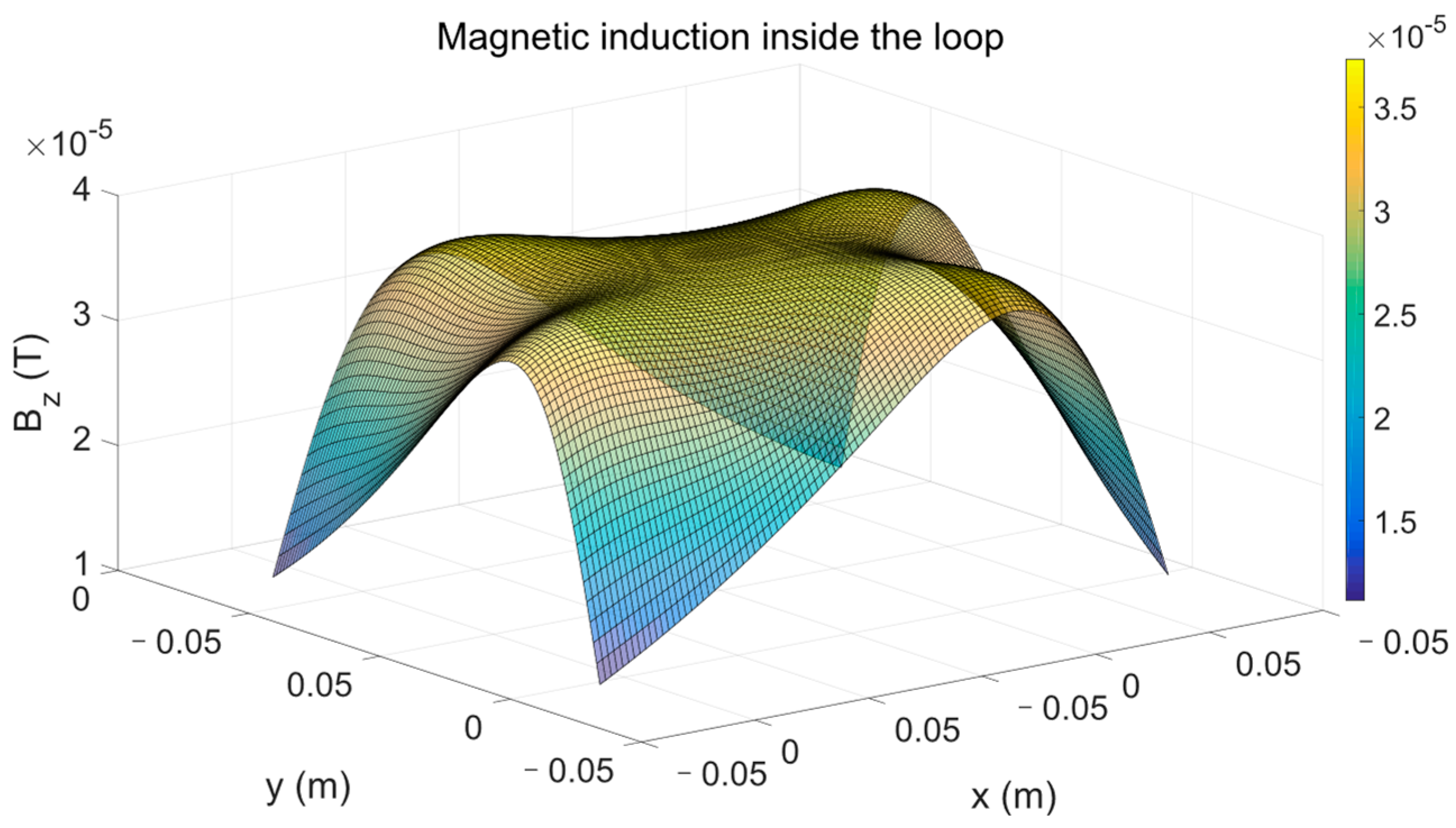
According to Equation (10), assuming that a 5A current is injected through a square transmitting antenna with a side length of 5 cm, the z-direction distribution of the magnetic induction is shown in Figure 6 at a horizontal plane with a distance of 2 cm from the antenna. Figure 6 shows that the magnetic field is approximately uniformly distributed within the projection of the induction loop.

According to the law of electromagnetic induction, the magnitude of the induced electromotive force e generated in a conductor loop is proportional to the rate of change $\mathrm{d}\mathsf{\Phi }$/$\mathrm{d}\mathrm{t}$ of the magnetic flux through the loop, i.e.,

$$\mathrm{e}=-{\displaystyle \frac{\mathrm{d}\mathsf{\Phi }}{\mathrm{d}\mathrm{t}}}=-{\displaystyle \frac{\mathrm{d}}{\mathrm{d}\mathrm{t}}}{\int }_{\mathrm{s}}\hspace{0.17em}\mathrm{B}·\mathrm{d}\mathrm{S},$$

(11)

according to the conclusion that the vertical component of the magnetic induction intensity inside the induction loop is approximately uniformly distributed, Equation (11) can be simplified as follows:

$$\mathrm{e}=-{\displaystyle \frac{\mathrm{d}\mathsf{\Phi }}{\mathrm{d}\mathrm{t}}}=-\mathrm{B}{\displaystyle \frac{\mathrm{d}\mathrm{S}}{\mathrm{d}\mathrm{t}}}.$$

(12)

In Equation (12), with a constant magnetic field generated by the transmitting antenna, the induced signal of the loop is only related to the effective projected area of the transmitting antenna in its plane. And the amplitude of the induced electromotive force is directly proportional to the movement distance of the antenna during a loop crossing cycle. Further, assuming that the distance between the center of the transmitting antenna and the nearest loop crossing point is d, the crossing cycle of the induction loops is l. The relationship between the peak-to-peak value of the induced voltage ${\mathrm{V}}_{\mathrm{p}\mathrm{p}}$ and d can be expressed as follows:

$${\mathrm{V}}_{\mathrm{p}\mathrm{p}}=\left\{\begin{array}{c}\mathrm{k}·\mathrm{d}, \mathrm{d}<{\displaystyle \frac{\mathrm{l}}{2}}\\ \mathrm{k}·(\mathrm{l}-\mathrm{d}), \mathrm{d}\ge {\displaystyle \frac{\mathrm{l}}{2}}\end{array}\right..$$

(13)

3.2. Analysis of Antenna Resonant Current and PWM Signal Duty Cycle

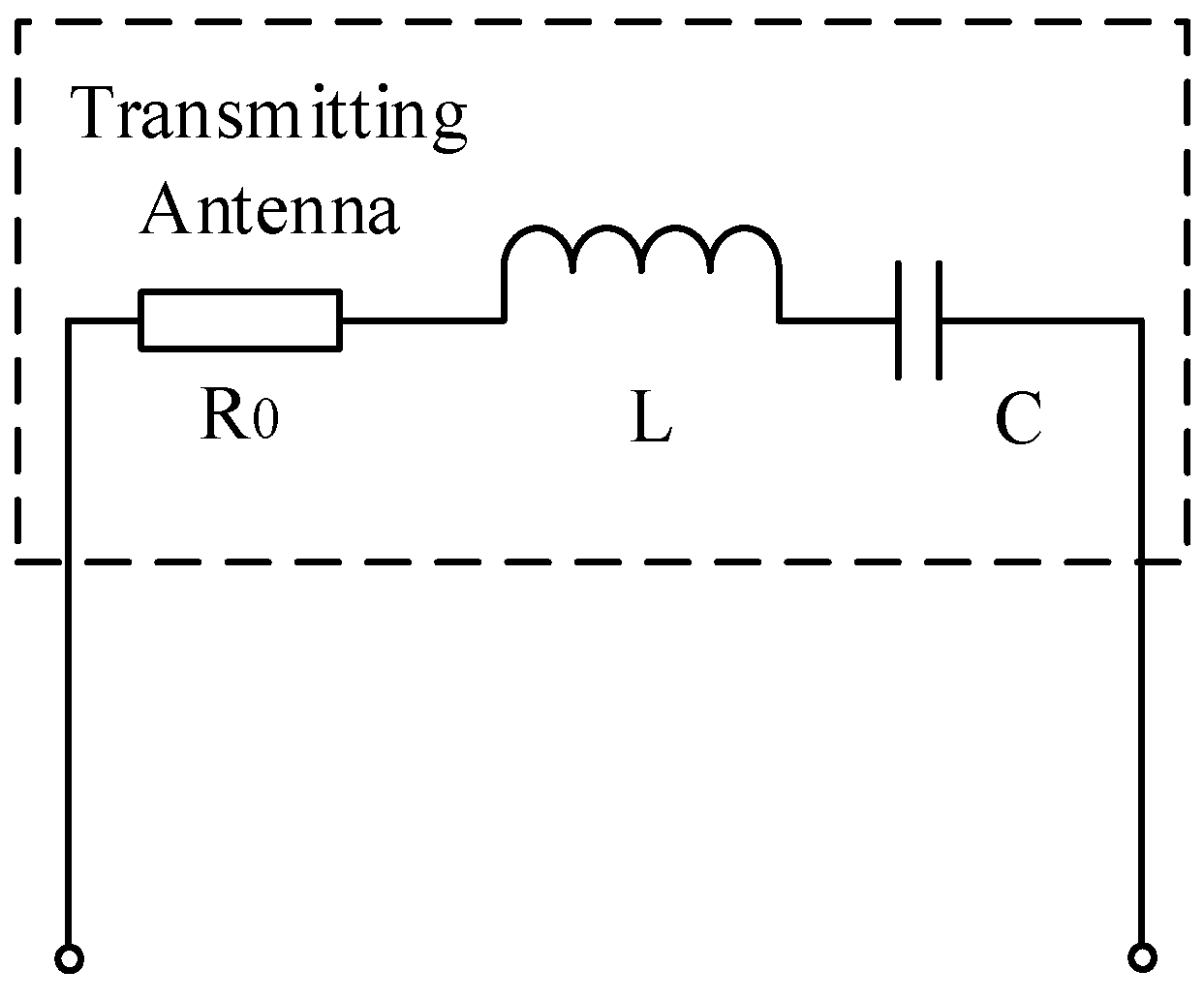
During the actual operation of the train, the amplitude of the induced signal in the loop will change periodically with the movement of the transmitting antenna, so the induced signal received in the corresponding loop can be simulated by adjusting the current of the transmitting antenna. The transmitting antenna is connected in series with a capacitor to form an RLC resonant circuit, and the circuit model can be approximated by the circuit of Figure 7.

The center frequency of the resonant circuit is the same as the frequency of the PWM, signal which is used as the excitation, and the current resonance of the circuit can be made by injecting the PWM signal into the circuit. By adjusting the duty cycle of the PWM signal, the magnitude of the resonant current in the transmitting antenna can be changed, thus changing the magnitude of the magnetic field generated by the transmitting antenna. To simulate the real operating conditions, the relationship between the resonant current amplitude and the duty cycle of the PWM signal is analyzed according to the RLC resonant circuit model.

For a periodic signal f(t) with period T, it is expressed as follows:

$$\mathrm{f}\left(\mathrm{t}\right)=\mathrm{f}(\mathrm{t}+\mathrm{k}\mathrm{T}),\mathrm{k}=\mathrm{1,2},3\dots \dots$$

(14)

This periodic function can be extended to an infinite series using trigonometric coefficients:

$$\mathrm{f}\left(\mathrm{t}\right)={\mathrm{A}}_0+\sum _{\mathrm{n}=1}^{\mathrm{\infty }}\hspace{0.17em}{\mathrm{A}}_{\mathrm{n}}\mathrm{s}\mathrm{i}\mathrm{n}\left({\displaystyle \frac{2\mathsf{\pi }}{\mathrm{T}}}\mathrm{n}\mathrm{t}+{\mathsf{\psi }}_{\mathrm{n}}\right),$$

(15)

i.e.,

$$\mathrm{f}\left(\mathrm{t}\right)={\mathrm{A}}_0+\sum _{\mathrm{n}=1}^{\mathrm{\infty }}\hspace{0.17em}\left[{\mathrm{a}}_{\mathrm{n}}\mathrm{c}\mathrm{o}\mathrm{s}\left({\displaystyle \frac{2\mathsf{\pi }}{\mathrm{T}}}\mathrm{n}\mathrm{t}\right)+{\mathrm{b}}_{\mathrm{n}}\mathrm{s}\mathrm{i}\mathrm{n}\left({\displaystyle \frac{2\mathsf{\pi }}{\mathrm{T}}}\mathrm{n}\mathrm{t}\right)\right].$$

(16)

The Fourier transform of the periodic signal f(t) is obtained by solving for ${\mathrm{A}}_0,{\mathrm{a}}_{\mathrm{n}},{\mathrm{b}}_{\mathrm{n}}$ according to the Fourier series expansion formula.

The PWM signal is used as the excitation source of the transmitting antenna, which is injected into the transmitting antenna and resonates to produce a high-frequency sinusoidal current signal in the antenna. The relationship between the amplitude of the resonant current and the duty cycle of the PWM signal is analyzed below. Let the PWM signal be a square wave signal with period T and duty cycle α:

$$\mathrm{f}\left(\mathrm{t}\right)=\left\{\begin{array}{c}\mathrm{A},\hspace{0.17em}\hspace{0.17em}\hspace{0.17em}0\le \mathrm{t}<\mathsf{\alpha }\mathrm{T}\\ 0,\hspace{0.17em}\hspace{0.17em}\hspace{0.17em}0\le \mathrm{t}<\mathrm{T}\end{array}\right.,$$

(17)

substituting into the expansion formula gives the following:

$$\left\{\begin{array}{c}{\mathrm{A}}_0={\displaystyle \frac{1}{\mathrm{T}}}{\int }_0^{\mathsf{\alpha }\mathrm{T}}\hspace{0.17em}\mathrm{A}\mathrm{d}\mathrm{t}=\mathsf{\alpha }\mathrm{A}\hfill \\ {\mathrm{a}}_{\mathrm{n}}={\displaystyle \frac{2}{\mathrm{T}}}{\int }_0^{\mathsf{\alpha }\mathrm{T}}\hspace{0.17em}\mathrm{A}\mathrm{c}\mathrm{o}\mathrm{s}\left({\displaystyle \frac{2\mathsf{\pi }\mathrm{n}}{\mathrm{T}}}\mathrm{t}\right)\mathrm{d}\mathrm{t}={\displaystyle \frac{\mathrm{A}}{\mathsf{\pi }\mathrm{n}}}\mathrm{s}\mathrm{i}\mathrm{n}(2\mathsf{\pi }\mathrm{n}\mathsf{\alpha })\hfill \\ {\mathrm{b}}_{\mathrm{n}}={\displaystyle \frac{2}{\mathrm{T}}}{\int }_0^{\mathsf{\alpha }\mathrm{T}}\hspace{0.17em}\mathrm{A}\mathrm{s}\mathrm{i}\mathrm{n}\left({\displaystyle \frac{2\mathsf{\pi }\mathrm{n}}{\mathrm{T}}}\mathrm{t}\right)\mathrm{d}\mathrm{t}={\displaystyle \frac{\mathrm{A}}{\mathsf{\pi }\mathrm{n}}}[1-\mathrm{c}\mathrm{o}\mathrm{s}(2\mathsf{\pi }\mathrm{n}\mathsf{\alpha })]\hfill \end{array}\right.\prime$$

(18)

In Equation (18), the fundamental wave amplitude is the largest. Since the RLC-series resonant circuit is a band-pass filter, if the fundamental frequency of the square wave is equal to the center frequency of the circuit, a resonant current of this frequency is generated between the inductor (i.e., the transmitting antenna) and the capacitor. The amplitude of this resonant current |A| is related to the PWM signal as follows:

$$\left|{\mathrm{A}}_{\mathrm{u}}\right|={\mathrm{A}}_1\times \mathrm{Q}=\sqrt{{\mathrm{a}}_1^2+{\mathrm{b}}_1^2}\times \mathrm{Q}={\displaystyle \frac{2\mathrm{A}}{\mathsf{\pi }}}\mathrm{s}\mathrm{i}\mathrm{n}(\mathsf{\alpha }·\mathsf{\pi })\times \mathrm{Q},$$

(19)

where A is the peak-to-peak value of the square wave signal and α is the duty cycle of the square wave signal. Q is the amplification (quality factor) of the RLC-series resonant circuit, which is related to the circuit parameters. Therefore, the amplitude of the sinusoidal voltage in the transmitting antenna is sinusoidally related to the duty cycle of the PWM signal. The change in voltage amplitude in the transmitting antenna can be adjusted by adjusting the duty cycle.

4. Implementation of the HIL Platform

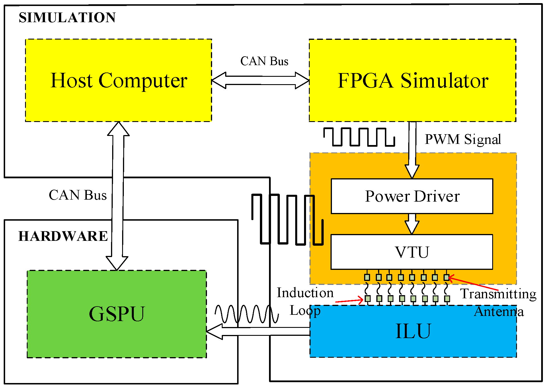
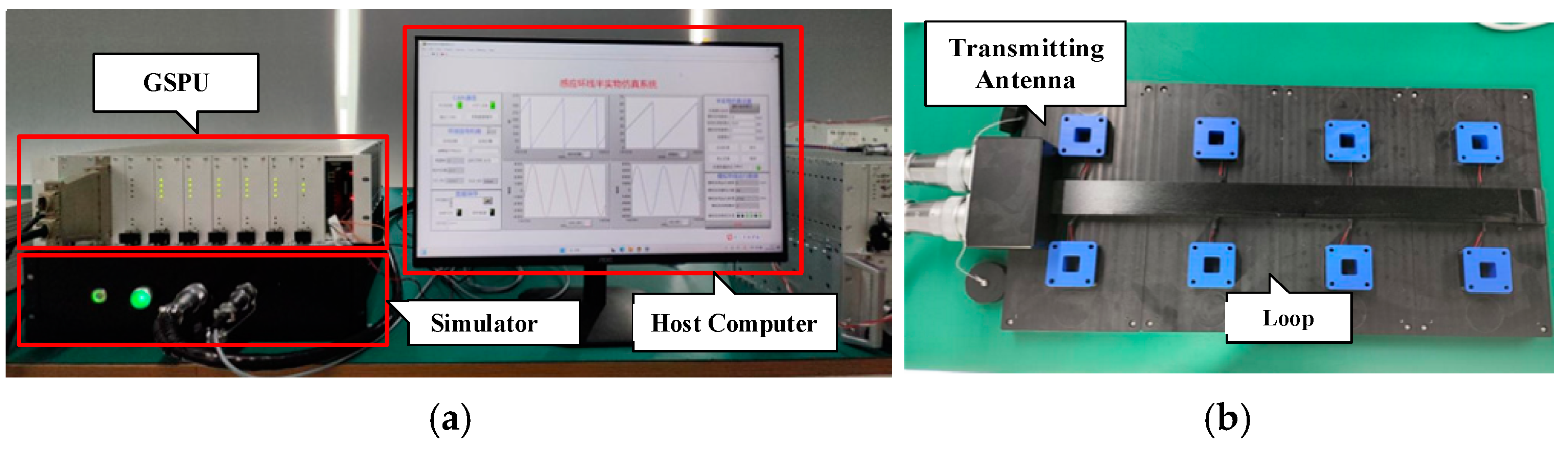
This HIL simulation platform is designed to validate the GSPU. The core task of the platform is validating the function and reliability of the GSPU by simulating the induced signal of the ILU when the train is in actual operation. In addition, the platform needs to have the ability to flexibly set the train operating parameters so as to simulate the signals received by ILU under different operating conditions and to enhance the wide applicability and practicality of the simulation test.

4.1. Platform Structure Design

The HIL simulation platform is composed of a host computer, an FPGA simulator, a resonant circuit, and the ILU, while the test object is the real GSPU. The platform is designed with eight groups of induction loops, each paired with a corresponding transmitting antenna, as illustrated in Figure 8. This multi-loop arrangement allows for spatially distributed signal generation, which is crucial for accurately mimicking the electromagnetic environment along the Maglev track.

Firstly, the simulation begins with the host computer, where parameters such as the train’s running mode, speed, acceleration, and other relevant dynamic conditions are preset. The FPGA simulator then uses these control parameters to compute the train’s instantaneous position in real time. This computation is essential for simulating realistic operational conditions and ensuring that the subsequent signal processing reflects actual train dynamics. Based on the calculated running position, the FPGA simulator computes the induced voltage signal for each induction loop in real time by applying Equation (13). This calculation considers the geometric and physical properties of the loops as well as the varying train positions, ensuring that the simulated signals closely replicate those that would be generated in a real environment.

Following the signal computation, the platform adjusts the PWM signal duty cycle for each transmitting antenna according to Equation (19). These PWM signals, once processed by the power driver, are injected into the VTU to simulate the induced signals that would be received by the ground-based loops. The proper calibration of these signals is vital for ensuring that the simulated electromagnetic fields accurately represent the conditions encountered by the GSPU.

The real GSPU, acting as the hardware under test, receives these simulated induced signals from the loops. It processes the data to extract critical information such as the relative and absolute position of the train and its running speed. The GSPU then transmits the processed information back to the host computer via the CAN bus, thereby completing the closed-loop system. This real-time feedback mechanism is instrumental for validating the performance and reliability of the system under simulated operating conditions.

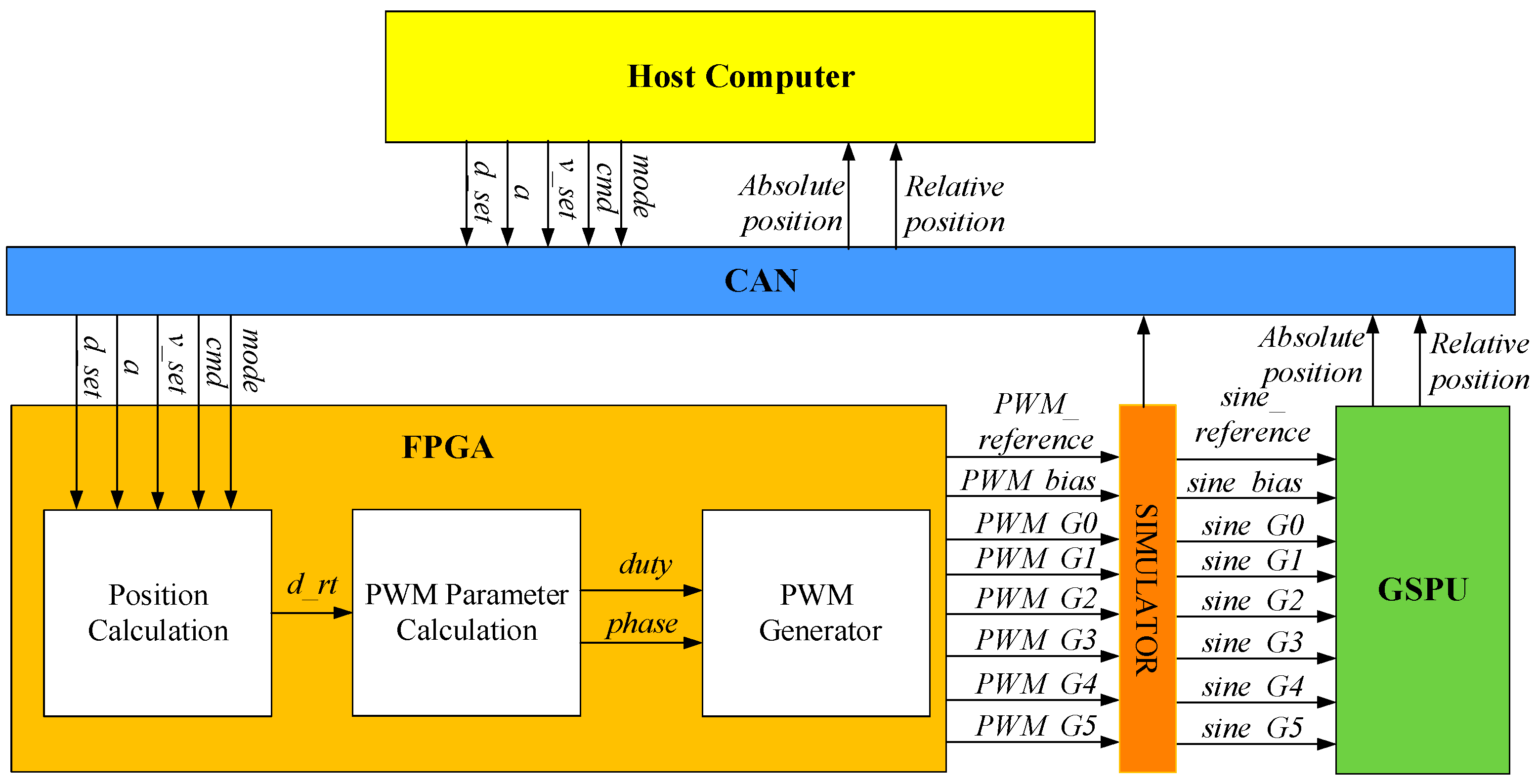
4.2. Platform Hardware and Software Design

The hardware of this platform includes an FPGA simulator, a power driver, and a VTU. The simulator is responsible for controlling each antenna, which requires high parallel computation capability. Therefore, the processing unit of the simulator adopts an FPGA. The simulator’s input is the simulated running position of the train, provided by the host computer, and its output is the PWM signal used to control the transmitting antennas. The power driver amplifies the PWM signal generated by the simulator, which is used to drive the transmitter antennas to generate a high-frequency alternating current.

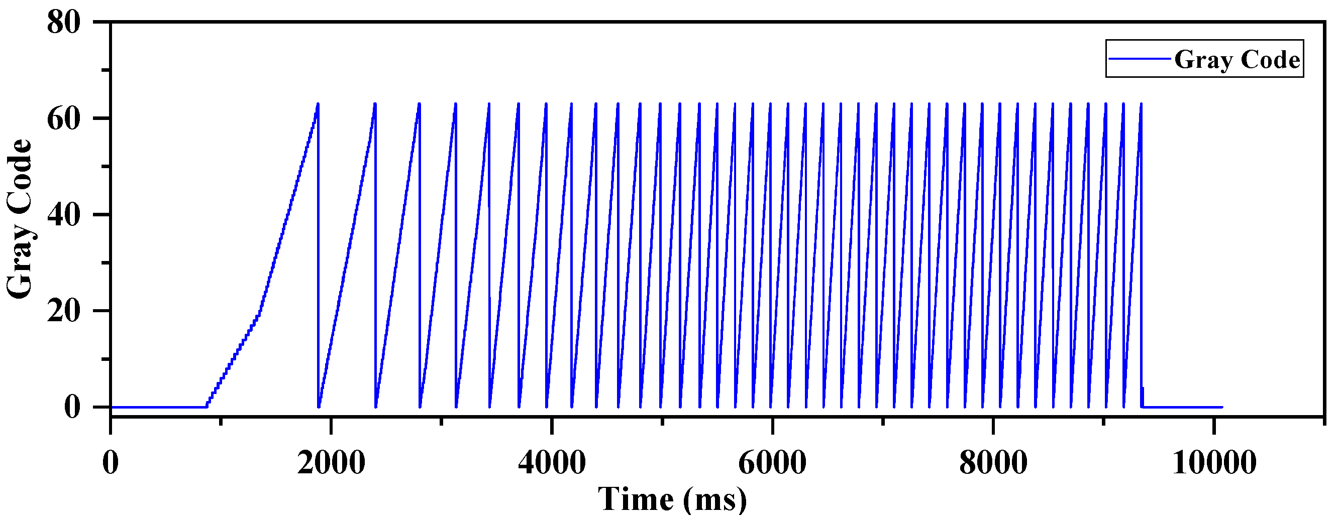
The software of this platform includes the host computer and the FPGA program of the processing unit in the simulator. The host computer uses a graphical display interface to control the start, pause, and stop of the simulation process, and the train motion can be set directly in the interface. The FPGA simulator calculates the train position in real time according to the train operation parameters. The simulation platform mainly simulates the three typical train operation modes, including the instantaneous position mode, the instantaneous speed mode, and the acceleration mode. The model needs to be implemented in FPGA, so it needs to be represented by differential equations to calculate the position and speed of the train in real time.

In the host computer, parameters such as the train operation mode, operation speed ${\mathrm{V}}_{\mathrm{s}\mathrm{e}\mathrm{t}}$, acceleration a, and the operation position ${\mathrm{D}}_{\mathrm{s}\mathrm{e}\mathrm{t}}$ can be set. These parameters are given to the FPGA simulator through the CAN bus. The following is an example of acceleration mode to give the differential equation of the running position of the train. In the accelerated motion mode, the train starts from position 0, performs a uniformly accelerated linear motion with the given acceleration a, and reaches the given maximum speed ${\mathrm{V}}_{\mathrm{s}\mathrm{e}\mathrm{t}}$ to keep the speed unchanged to perform a uniform linear motion. The differential equation with respect to the train running position $\mathrm{D}\left[\mathrm{n}\right]$ is expressed as follows:

$$\left\{\begin{array}{c}\mathrm{D}\left[\mathrm{n}+1\right]=\mathrm{D}\left[\mathrm{n}\right]+{\mathrm{V}}_{\mathrm{n}}\times \Delta \mathrm{t}, \mathrm{V}\le {\mathrm{V}}_{\mathrm{s}\mathrm{e}\mathrm{t}}\\ \mathrm{V}\left[\mathrm{n}+1\right]=\mathrm{V}\left[\mathrm{n}\right]+\mathrm{a}\times \Delta \mathrm{t},\mathrm{V}\le {\mathrm{V}}_{\mathrm{s}\mathrm{e}\mathrm{t}}\\ \mathrm{D}\left[\mathrm{n}+1\right]=\mathrm{D}\left[\mathrm{n}\right]+{\mathrm{V}}_{\mathrm{s}\mathrm{e}\mathrm{t}}\times \Delta \mathrm{t}\\ \mathrm{V}\left[\mathrm{n}\right]=0,\mathrm{D}\left[0\right]={\mathrm{D}}_{\mathrm{s}\mathrm{e}\mathrm{t}}\end{array}\right..$$

(20)

The operation of the simulation system is shown in Figure 9. The train operation mode and parameters are set in the host computer, and the FPGA reads these parameters through the CAN bus and solves the above differential equation in the position calculation module to obtain the real-time running position of the train, d_rt. 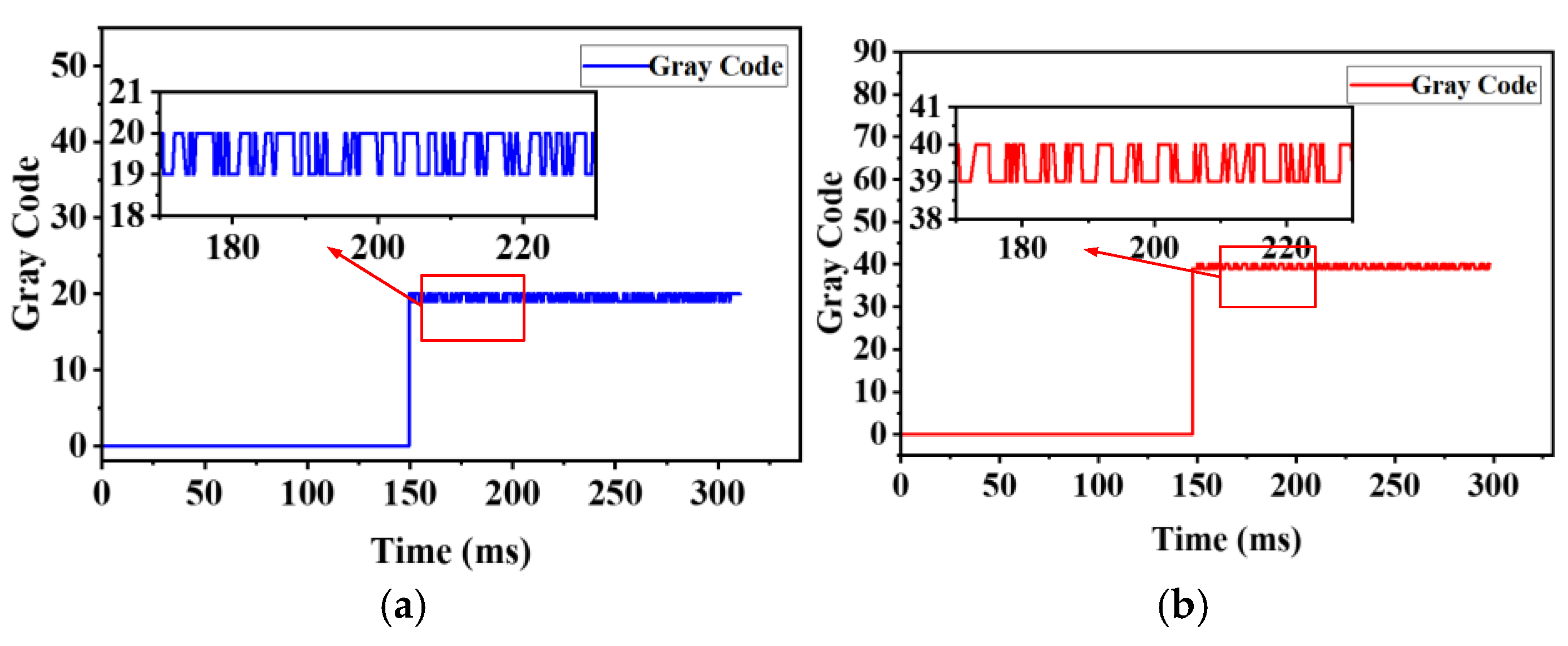The PWM parameter calculation module calculates the duty cycle and phase of the PWM wave of each transmitting antenna according to d_rt. At the same time, the host computer centrally displays the simulated running position and the position information processed by the GSPU. The relative position, absolute position, and the Gray code are displayed in the form of curves in the host computer interface. By comparing whether the two are consistent or not, it can be verified whether the processing function of the ground unit is correct or not. The host computer can also save the simulation data to further analyze the operation of the GSPU.

5. Results

To evaluate the effectiveness of the proposed HIL simulation platform, a series of experiments were conducted focusing on the physical implementation and functional verification of the system. This section presents the results obtained from the constructed platform and analyzes the performance of the GSPU under different operating conditions.

5.1. Physical Construction of Platforms

The HIL simulation platform consists of four parts, which are the host computer, the simulator, the real GSPU chassis, and the signal receiving unit. Among them, the signal receiving unit includes eight transmitting antennas and eight groups of induction loops, as shown in Figure 10.

The HIL simulation platform is run in the instantaneous speed mode, the instantaneous position mode, and the acceleration mode, respectively. The corresponding parameters are shown in

Table 2. Parameters set by the HIL simulation platform. The physical parameters and parameters for train operation in three modes are included.

Parameter Item		Parameter Setting
physical parameters	transmitting antennas	$l=5 \mathrm{c}\mathrm{m},I=5 \mathrm{A}$
	induction loops	$h=2 \mathrm{c}\mathrm{m},crossing period=50 \mathrm{m}\mathrm{m}$
operating parameters	instantaneous speed mode	$D_{set}=0,V_{set}=5 \mathrm{m}/\mathrm{s}$
	instantaneous position mode	$1.D_{set}=1000 \mathrm{m}\mathrm{m};2.D_{set}=2000 \mathrm{m}\mathrm{m}$
	acceleration mode	$V_{set}=0,D_{set}=0;a=1 {\mathrm{m}/\mathrm{s}}^2;$ $V_{set}=10 \mathrm{m}/\mathrm{s}$

.

Table 3. FPGA resource occupancy statistics. It lists several typical resource occupancy rates.

Software Modules	LUT	Flip-Flop	Block RAM
Analog position calculation	1.19%	0.08%	0.41%
Calculation of PWM parameters	1.48%	0.21%	0.58%
PWM signal generation	0.43%	0.15%	0.78%
Communication	3.73%	1.73%	1.38%
Totals	6.83%	2.17%	3.15%

shows the resource occupancy of different software modules in the FPGA. It shows that the communication module occupies the highest resource occupancy, and the calculation and generation of the PWM signal parameters of the transmitting antenna occupy a smaller resource occupancy, indicating that the simulation strategy based on parallel signal simulation is effective.

5.2. Functional Verification

5.2.1. Instantaneous Speed Mode Analysis

In the instantaneous speed mode, the train starts from position 0 and moves at a constant speed according to the set running speed. The relative position and absolute position information processed by the GSPU can be observed in the host computer interface. To facilitate the display of the absolute position, the GSPU decodes the Gray code into BCD code and finally displays it in the form of decimal in the host computer interface. Figure 11 shows that the Gray-code information of the train position is incremented from 0 to 63 and then becomes 0 again and keeps cycling as expected. Each Gray code then corresponds to a Gray-coded period of the ground loop to represent the absolute position of the train.

The relative position is calculated based on the division of the amplitude of the induced signal of the lowest address loop G0 and the bias loop SG0. The amplitude of the G0 and SG0-induced signals output from the GSPU is shown in Figure 12, which is approximated as two sinusoidal signals with a phase difference of 90°. This is consistent with the results analyzed in Figure 4.

The relative position change curve obtained from the processing of the G0 and SG0 induced signals is shown in Figure 13. The curve approximates a sawtooth wave and varies between 0 and 360°, indicating the relative position change of the train within a loop cell, as expected.

According to the absolute position and relative position information obtained from processing, the running position can be calculated. Compared with the simulated distance and speed sent by simulator, it is found that the two are consistent, which indicates that the HIL simulation platform can correctly simulate the operating environment of the GSPU.

5.2.2. Instantaneous Position Mode Analysis

In the instantaneous position mode, the stationary position of the Maglev train is set. Regarding when the position is set to 1000 mm or 2000 mm, the absolute position information is shown in Figure 14. As the Gray-coded period of the loops is 50 mm, when the train is at 1000 mm, it is located at the 20th Gray code of the loop, i.e., the BCD code corresponding to the absolute position Gray code is 20. As the train is directly above the crossing point of the loop, the absolute position code jumps between 19 and 20. Similarly, when the train is at 2000 mm, the absolute position code jumps between 39 and 40, as expected.

5.2.3. Acceleration Mode Analysis

In the acceleration mode, the Maglev train starts from position 0, accelerates uniformly with an acceleration of $1 \mathrm{m}/{\mathrm{s}}^2$, and runs at a uniform speed after the speed reaches $10 \mathrm{m}/\mathrm{s}$. The result is shown in Figure 15, where the change of the Gray code information representing the absolute position of the train is gradually accelerated. Until the train starts to move at a uniform speed, at which point the curve becomes stable, as expected.

5.3. Analysis of Experimental Results

To analyze the errors generated by the GSPU in the HIL simulation platform, the platform was run in instantaneous speed mode at $50 \mathrm{k}\mathrm{m}/\mathrm{h}$, $200 \mathrm{k}\mathrm{m}/\mathrm{h}$, and $600 \mathrm{k}\mathrm{m}/\mathrm{h}$. Then the platform was run in acceleration mode with accelerations of $1 \mathrm{m}/{\mathrm{s}}^2$, $2 \mathrm{m}/{\mathrm{s}}^2$, and $3 \mathrm{m}/{\mathrm{s}}^2$, respectively, in which the train maintains a uniform speed after 30 s of acceleration. The positioning and speed measurement information obtained from the GSPU is exported. The error analysis in the instantaneous position mode was not included in the statistics because it was not informative.

The positioning error during uniform and accelerated motion is shown in Figure 16. It shows that the positioning error stabilizes at a constant millimeter level when the train speed is constant. Besides, when the train running speed increases, the positioning error increases slightly. This is because the positioning uses a combination of absolute and relative positions, and the position information is corrected each Gray-coded period. As a result, the accuracy of the position information can reach the millimeter level, and the cumulative error is eliminated. The positioning error increases slightly when the running speed is too high, which is related to the processing speed of the simulator and the sampling rate of the GSPU.

The speed measurement error during uniform and accelerated motion is shown in Figure 17. It shows that the speed measurement error is related to the running speed of the train. The faster the speed, the larger the absolute error of speed measurement. However, from the point of view of relative error, when the running speed is 50 km/h, the relative error of speed measurement is about 2.14%. When the running speed is 600 km/h, the relative error of speed measurement is about 1.06%. When the train is running steadily, the fluctuation of the speed measurement error is also very small. This is also related to the speed measurement method, in which the GSPU is obtained by calculating the ratio of the distance Δd between two adjacent crossing nodes of the loop and the elapsed time Δt. This method effectively ensures the accuracy of speed measurement at low speeds. At the same time, when the speed increases, the elapsed time between adjacent intersections becomes shorter, and the absolute error of the speed measurement increases slightly, but the relative error decreases, which is in line with expectations.

Table 4. Positioning and speed measurement errors.

Speed	Average Error
	Positioning (mm)	Speed Measurement (km/h)
50 km/h	1.47	1.07
200 km/h	1.92	3.19
600 km/h	2.58	6.34

shows the average error in positioning and speed measurements at low, medium, and high speeds for 20 runs. Even in the high-speed condition, the positioning error is only 2.58 mm, and the speed error is 6.34 km/h. The results show that the HIL platform can effectively simulate the various operation modes of high-speed Maglev trains and provide a reliable test environment for the GSPU. And the experiment also verifies the reliability and integrity of the GSPU function.

6. Discussion

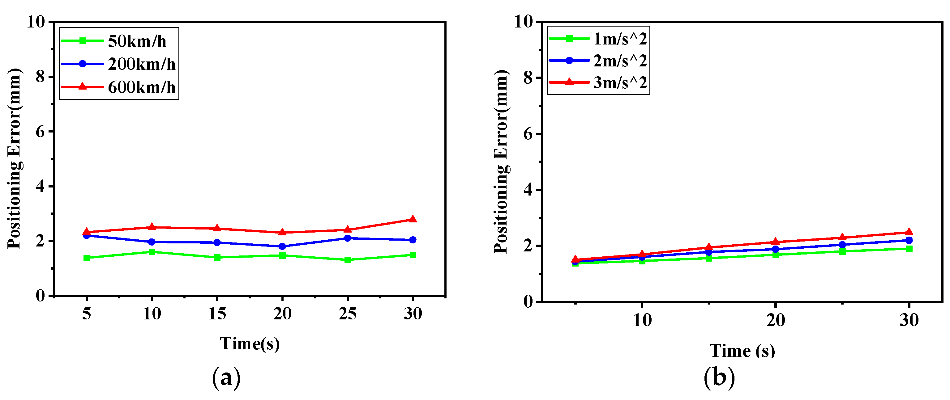
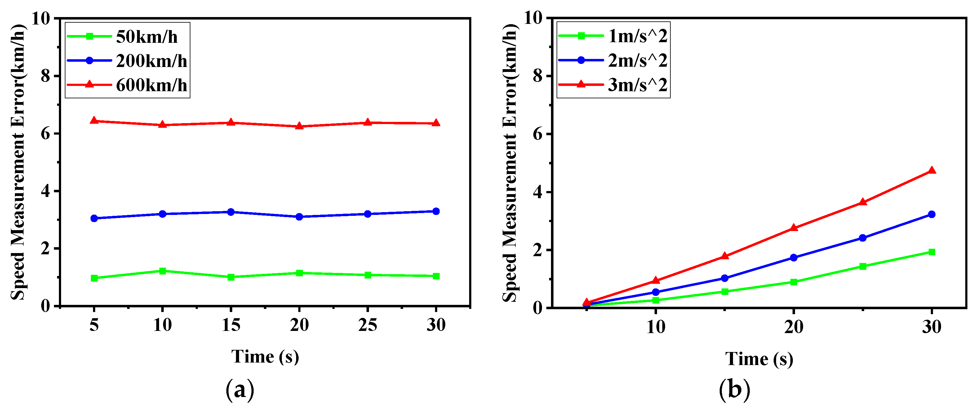
In this paper, an HIL simulation platform based on induction loops is built to solve the verification problem at the early stages of MPSS development. Firstly, a positioning method combining the absolute position and the relative position is proposed, and the principles of the two position detection methods are explained. The calculation process of key signals in MPSS is analyzed, and a simulation strategy based on parallel signal reconstruction is adopted. Based on this, the HIL simulation platform is built for the GSPU, which is the core of MPSS. Finally, experimental validation of the GSPU is carried out on this platform. The experimental results show that the HIL simulation platform is effective. It can accurately verify the positioning and speed measurement function of the GSPU in various operation modes of high-speed Maglev trains. Meanwhile, under the high-speed condition of 600 km/h, the positioning error of the GSPU is only 2.58 mm, and the speed measurement error is 6.34 km/h. It validates the effectiveness of the positioning and velocity measurement method proposed in this paper.

Since the Gray-coded loops are inducing voltage signals through electromagnetic fields, they are inevitably exposed to an electromagnetic interference environment. To address this, the GSPU has taken effective measures at both the hardware and software levels. For example, the current frequency of the transmitting antenna is much higher than that of the traction motor, filtering is performed at the hardware level, and particle filtering algorithms are used at the software level. In addition, in order to expand the potential of the platform and adapt to a variety of operating modes, the train position algorithm of the HIL platform will be optimized in the future. By introducing the real speed curve when the Maglev train is running, the whole operation mode of the train can be set flexibly to realize the simulation of different operation scenarios. What is more, the expansion interface is reserved in the platform, which provides the possibility of integrating the multi-train collaborative test as well as verifying the anti-interference performance of the GSPU in the future. This lays a solid foundation for subsequent research and the diversification of applications. For the functional testing of other parts of the MPSS, such as the transmitting antenna, it is recommended to build a motion simulation platform to carry this out.