Optimizing Teleconsultation Scheduling with a Two-Level Approach Based on Reinforcement Learning

Abstract

Using advanced communication and information technologies, teleconsultation can provide high-quality healthcare services to remote areas. To enhance service efficiency, this study develops a two-level dynamic scheduling model for teleconsultation, which prioritizes optimizing service frequency and incorporates downstream room utilization and overtime risk as considerations. The first-level model is a data-driven framework that optimizes the frequency by adjusting service start times. Based on the solutions of the first-level model, a second-level model is built to assign teleconsultation rooms to departments with demands and reduce the total overtime risk and and room opening cost. For solving, an integer programming (IP) solver is embedded in a deep reinforcement learning (DRL) approach. A presorting mechanism of interval constraints is proposed to improve the quality of solutions. For verification, actual teleconsultation data are used as samples. The experimental results demonstrate the effectiveness of the proposed two-level model, the embedded solving algorithm, and the interval constraint presorting mechanism. Compared with real schedules, the two-level model can reduce four service scheduling performance criteria, including demand average waiting time, number of services, risk of overtime, and number of rooms used. As a result, the efficiency of teleconsultation is improved to promote its development.

1. Introduction

Using advanced information and communication technologies to deliver healthcare services remotely, telemedicine is a potential solution to improve access to healthcare and reduce healthcare costs [1,2]. In China, B2B teleconsultation is the most used telemedicine service, proving highly effective in mitigating the uneven distribution of high-quality medical resources. Via videoconferencing, primary hospitals gain access to the specialist resources of class-A tertiary hospitals, thereby enhancing the quality of medical services. Having been rolled out across 29 provinces, teleconsultation has benefited a vast number of patients [3].

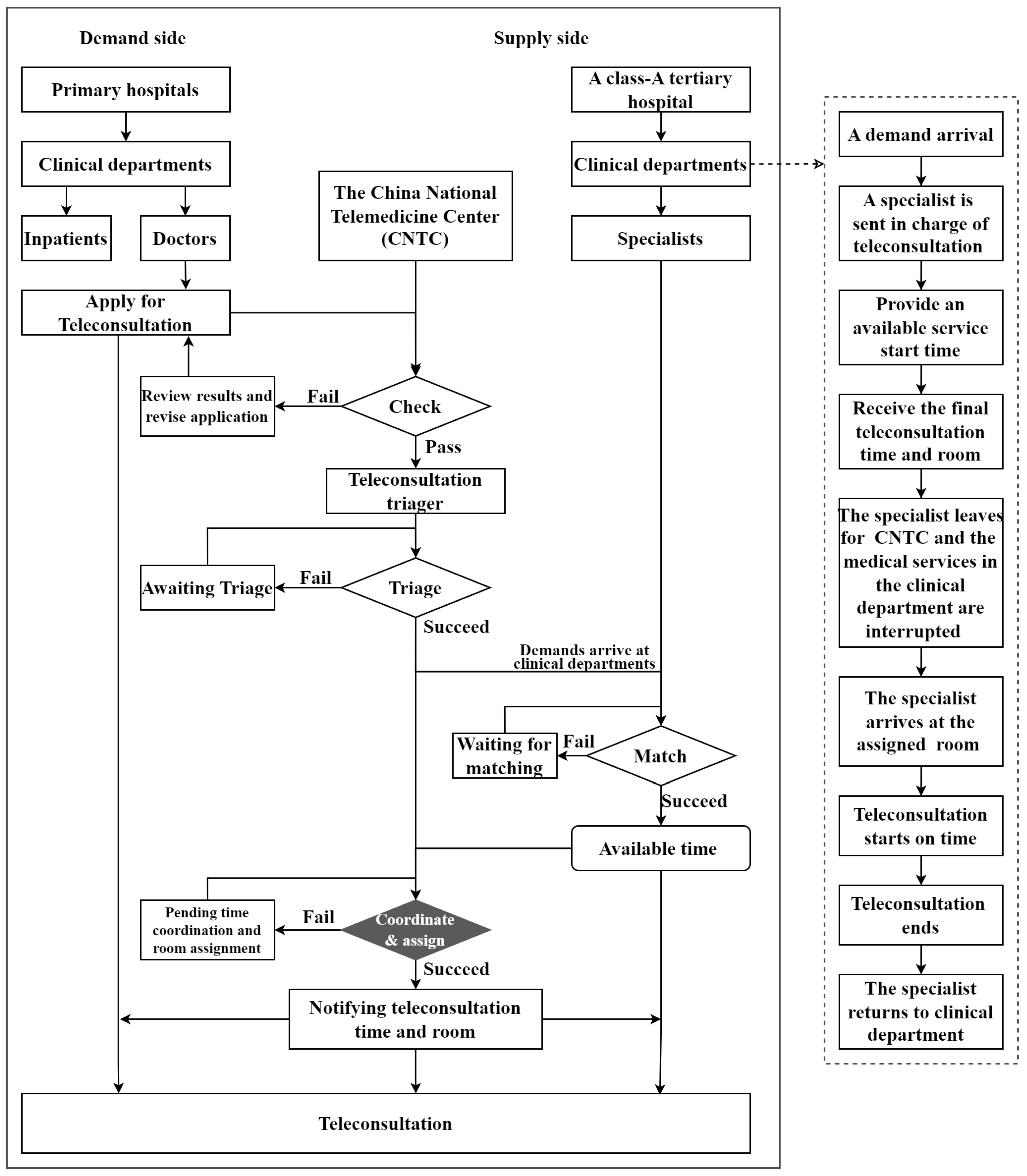
The characteristics of teleconsultation can be summarized as follows: it shares a similar service duration with outpatient services and has comparable room requirements to surgical services. However, it is also distinguished by three notable features: the involvement of four participants, service mobility, and intermittent demand. The four participants include doctors and inpatients in primary hospitals (demand side), and the China National Telemedicine Center (CNTC) and specialists in a class-A tertiary hospital (supply side), as shown in Figure 1. Service mobility refers to the fact that specialists do not hold fixed office hours or reserve dedicated rooms for teleconsultations. Instead, they move from their clinical departments to CNTC to deliver teleconsultation services, as elaborated in the dashed-line block diagram of Figure 1. Service mobility stems, on the one hand, from the specific requirements for teleconsultation, including devices, networks, and management, which are met at the CNTC. On the other hand, the lack of specialists dedicated exclusively to teleconsultations can be attributed to intermittent demand and short service durations. Intermittent demands did not cause system congestion issues. The average duration is about eight minutes [4]. Specialists are only assigned to deliver teleconsultation services when a teleconsultation request is received.

Figure 1. A schematic of the teleconsultation process.

Owing to the characteristic, the operational challenges of teleconsultation are more complex than those of traditional healthcare services. For instance, when modeling the specialist assignment problem, Ji et al. [5] incorporated three distinct sources of uncertainty, including uncertain service durations and no-show behaviors from both the demand and supply sides. Regarding the allocation and scheduling of teleconsultation resources, clinical departments are integrated and grouped into five medical sections to mitigate the issue of intermittent demand [6,7]. In terms of the daily scheduling problem with a single teleconusltation server, Wan et al. [8] considers the mobility of the specialist doctor and the time anxiety of primary doctors to build an approximate semidefinite programming model to reduce the risk level of overtime and waiting cost. Considering service mobility and demand intermittency, Chen and Li [9] build a dynamic scheduling model for teleconsultation to optimize its start time to reduce long-term service cost. In the model, the objective includes the number of service times of specialists. Although a smaller number of service times can reduce the service cost, blindly pursuing a smaller number of it can lead to a high risk of overtime [10].

To avoid long overtime, this study considers the adjustment of service start time to reduce the risk of overtime in teleconsultation. Furthermore, time also needs to be coordinated to assign rooms, seen in the highlighted black filled diamond in Figure 1. To our best knowledge, these have not been analyzed in the consideration of optimizing service frequency. Frequent teleconsultation services result in numerous round trips for specialists between clinical departments and the CNTC, wasting their time, undermining the quality of on-site medical services, and reducing the efficiency of teleconsultations. This is not conducive to the sustainability of teleconsultation with intermittent demands. Therefore, to fill the gap, optimizing service frequency is designated as a priority objective, with overtime risk and downstream teleconsultation room usage considered as secondary factors in the problem. For this purpose, we build a two-level approach for teleconsultation scheduling optimization. The first level is the dynamic start-time optimization model built by [9], of which the objective includes reducing the service frequency. Room assignment and start time adjustment models are built based on each output of the first model, resulting in a main dynamic model embedded with multiply branch models. This two-level structure can avoid the decline in model solving efficiency caused by high-dimensional action sets. The dimension of action sets increases severalfold when optimizing service start time and allocating rooms simultaneously. For problem solving, deep reinforcement learning (DRL) and integer programming (IP) solver are combined to form an embedded algorithm. The applied data are actual records including the arrival time for the teleconsultation demand and the arranged start time of the service with a long-term observation of several months. The results demonstrate the effectiveness of the proposed approach and algorithm.

The remainder of this paper is structured as follows. Section 2 reviews the relevant literature and elaborates on our contributions. Section 3 and Section 4 first describe and formulate the research problem, and then introduce the solution approaches. Section 5 and Section 6 present the experimental design, results, and discussions. Finally, Section 7 concludes the paper and outlines directions for future research.

2. Literature Review

The related literature is reviewed from three aspects: studies on telemedicine or teleconsultation scheduling, the two-level scheduling models used in healthcare, and the application of reinforcement learning in solving two-level models.

2.1. Teleconsultation Scheduling

Previous studies on telemedicine or teleconsultation scheduling can be categorized into four types. The first type focuses on the scheduling of online demands, such as chronic patients’ online consultation [11], of which the service pattern is different from teleconsultation. Regarding the second type, three studies explore both the integration of virtual patients and the effects of virtual visits [12,13,14]. Their research scope is more macro-level compared to scheduling studies on healthcare services. For the third type, three studies study the outpatient scheduling problem considering both online and offline demands [15,16,17]. Although these studies consider online demands, they focus on optimizing the scheduling of outpatient service patterns. The outpatient service differs from the teleconsultation service in its fixed office hours and room. Teleconsultation has an irregular start time and multiple departments share a room like a surgery service. The fourth type of research comprises five studies on teleconsultation scheduling problems that are most related to this study. The similarities and differences of these studies with our study are compared in Table 1.

Table 1. Comparison of the relevant literature about teleconsultation scheduling.

Papers	Methods *	Objective	Duration	Department Setting
[7]	DES	Average waiting time	Long term	Merger into five
		Variance in waiting time		medical sections
		Completed numbers
[18]	ML, TM, SP	The revenue of scheduling	Four hours	Not considered
		patients and doctors,
		postponing patients,
		overtime, and cancellation
[10]	SP, MIP	Room use	Long term	Actual setting
		Overtime cost
[8]	DRO	The total cost considering	One day	A neurology
		doctors’ and an inpatient’s		department
		waiting
[19]	SP	Unallocated penalty costs	Long term	Megered into five
		Waiting costs		medical sections
		Idle costs
		Overtime costs
[9]	DRL	Waiting time	Long term	Actual setting
		Specialist service cost		Multiple departments
This paper	DRL, MIP	Waiting time	Long term	Actual setting
		Specialist service cost		Multiple departments
		Room use
		Overtime risk

* DES: discrete-event simulation; ML: machine learning; TM: text mining; SP: stochastic programming; MIP: mixed-integer programming; DRO: distributionally robust optimization; DRL: deep reinforcement learning.

Our study differs mainly from the relevant studies in terms of applied method, optimization objective, duration, and department setting. From a data-driven perspective, we propose a two-level approach for teleconsultation scheduling optimization. The applied methods include DRL and IP. DRL is used to solve the first-level problem of start time optimization of teleconsultations, which is proposed in [9]. Based on the teleconsultation start time optimization, IP is used to further consider the downstream room use and overtime risk in the scheduling problem. For the modeling duration, we consider a long term of monthly cost consisting of four parts, i.e., the demand waiting time, specialist service cost, room opening cost, and overtime risk. For validation purposes, we adopt the actual departmental structure without any integration, and multiple clinical departments are selected as samples for our experiments.

2.2. Two-Level Scheduling Models in Healthcare

Two-level models or two-stage models have been used to solve various scheduling problems in healthcare, including medical staff allocation and scheduling [20], operating room scheduling [21], outpatient scheduling [22,23], surgery scheduling [24], supply chain scheduling [25,26], and medical training scheduling [27]. All of these problems have multiple decisions to be made, or the decisions have multiple phases. For example, Azaiez et al. [21] developed a two-stage no-wait hybrid flow shop scheduling model with inter-stage flexibility for operating room scheduling under limited service resources, aiming to optimize the timing of each step in the surgical process. Zhang et al. [24] proposed a novel two-phase optimization model that integrates the Markov decision process with stochastic programming to enhance the long-term performance of surgical schedules. This model determines which surgical blocks to open for the following week and assigns a subset of waiting-list surgeries to these blocks. Batuhan et al. [23] formulated a two-stage stochastic mixed-integer nonlinear programming model to allocate patient treatments to specific days within a multi-week planning horizon and schedule their appointment times for the assigned day.

Two-level models have advantages in modeling complex scheduling problems considering the interaction of different phases or the collaboration of limited resources. For example, Li et al. [22] built a two-phase service model and obtained a joint scheduling policy to determine appointment times for two types of patients. The joint scheduling policy can reduce the waiting time for all patients and improve the efficiency of the system at the same time. Wang et al. [20] proposes a two-stage robust model to consider collaborations in which the surgeon of one surgery might be assigned as the assistant of another surgery. Surgery allocations and surgeon assignments are determined first, and then the start time of each surgery is decided.

For teleconsultation, the process flowcharts described in [7,8,9,19] show that there are multiple decisions to complete a teleconsultation, and some of the decisions are interactive, such as the start time of teleconsutlations and the room assignment for them. Therefore, this study proposes a two-level model to optimize these two decisions considering the interaction between them.

2.3. The Application of Reinforcement Learning in Solving Two-Level Models

Reinforcement learning has advantages in solving complex problems due to efficient data use and the adaptability to different problems [28,29]. To flatten the aggregate load on the power grid and reduce peak demand, Zhao et al. [30] proposes a two-level hierarchical charging scheduling model. This model is solved by a DRL approach that combines deep Q-network and deep deterministic policy gradient to handle the hybrid action space with both discrete and continuous actions. To solve the problem of scheduling a two-stage hybrid flow shop, Xu et al. [31] design an adaptive objective selection-based Q learning algorithm. The algorithm utilizes real-time data about jobs, machines, and waiting processing queues to achieve coordinated optimization for multiple objectives. To simultaneously determine the planning of lot sizing and the scheduling of the production sequences, Jabeur et al. [32] propose an integrated lot sizing and flexible flow line production scheduling model, which is solved by a two-level approach relying on reinforcement learning. For teleconsultation, the problem of start time optimization has been solved by a DRL, which is developed according to the demand intermittency in [9]. The DRL has been shown to outperform the actuality and the traditional value iteration method. Therefore, the DRL is applied as the base to solve the two-level model.

3. Problem Modeling

In constructing the models, this section first provides a brief description of the scheduling problem, followed by an introduction to the models at both the first and second levels.

After the clinical department provides the available service time, CNTC considers the available time of teleconsultation rooms to decide the final service start time and assign the service room. The start time are modeled and optimized in [9]. Based on these models, this study constructs room assignment models, resulting in a two-level approach. For modeling, the priority of emergency is not considered for departments because emergency teleconsultation services are provided by the emergency department, which is not included in the current research sample. The demands of a department are serviced following the rule of first-come and first-service (FCFS) due to non-emergency.

3.1. The First-Level Model

The first-level model is used to optimize the teleconsultation start time of each clinical department. The notation are defined in Table 2 and formulations are presented below.

Table 2. The notation for the formations of first-level model.

Types	Notation	Defines
Set	$\mathcal{D}$	The available time
	$\mathcal{M}$	Departments providing teleconsultation services $\left\{1,...,m,...,M\right\}$
	$\mathcal{I}$	The total amount of teleconsultation demands of clinical departments $\left\{I_1,...,I_m,...I_M\right\}$
Subscript	m	Department indexing
Superscripts	i	Teleconsultation demand $i=1,...,I_m$
	j	Teleconsultation service $j=1,...,J_m$
Variables	$t_m^i$	Arriving time of the demand i of department m
	$w_m^i$	Waiting time of the demand i of department m
Parameters	$\alpha$	The unit service cost
	$\beta$	The time interval between two consecutive teleconsultations
Decision variables	$d_m^j$	The start time of the jth service of department m

From a data-driven perspective, we aim to optimize the start times of teleconsultations by constructing a general teleconsultation scheduling model based on the empirical cost minimization principle. Specifically, using a dataset collected over an observation period, the model seeks to learn an optimal decision function $f^{*}$ that minimizes the value of the service cost function L. Mathematically, this is expressed as $f_m^{*}=arg{min}_{f_m\in F}L(w_m^1,...,w_m^{I_m},d_m^1,...,d_m^{J_m};\alpha )$. In our study, L specifically consists of demand waiting costs and service provision costs, as detailed in Equation (1).

$$min\left(\sum _1^{I_m}{w}_m^i+\alpha ·J_m\right).$$

(1)

Subject to:

$$w_m^1=d_m^1-t_m^1,i=1,$$

(2)

$$\begin{array}{c}\hfill w_m^i=\left(d_m^1-t_m^i\right)\mathbb{I}\left(d_m^1-t_m^i\right)+\sum _{j=2}^i\left(d_m^j-t_m^i\right)·\mathbb{I}\left(-\left(d_m^{j-1}-t_m^i\right)\left(d_m^j-t_m^i\right)\right),\\ \hfill i=2,...,I_m,\end{array}$$

(3)

$$J_m\le I_m,\alpha >1,\beta >0,$$

(4)

$$d_m^{j+1}-d_m^j\ge \beta ,d_m^{j+1}\in \mathcal{D},d_m^j\in \mathcal{D},j=1,2,...,J_m-1.$$

(5)

The first-level model incorporates five constraints. Constraints (2) and (3) calculate the demand waiting time by using an indicator function, $\mathbb{I}\left(a\right)=\left\{\begin{array}{cc}1,& a\ge 0,\\ 0,& a<0.\end{array}\right.$ Constraint (4) defines the feasible ranges of specific parameters. $J_m\le I_m$ denotes that the total number of teleconsultations provided is less than or equal to the total number of demands. This is understandable because one teleconsultation is provided for at least one demand. $\alpha >1$ indicates that the unit service cost of specialists exceeds the unit waiting cost of demands, a reasonable setting given the scarcity and high value of specialist resources. $\beta >0$ imposes a non-zero time interval between two consecutive teleconsultations, as formalized in constraint (5). The model defined by Equations (1)–(5) are built for department m. Since $m\in \mathcal{M}$, there are M scheduling models in the first level. Each model can be converted into a Markov decision process and then solved by the deep reinforcement algorithm proposed in [9] to output the optimized start time of the corresponding department.

3.2. The Second-Level Model

The second-level model is a room assignments model. The notation are defined in Table 3.

Table 3. The notation for the formations of second-level model.

Types	Notation	Defines
Set	${\mathcal{A}}^t$	The t available working period for teleconsultation service ${\mathcal{A}}^t\in \mathcal{D}$, in which there are N discrete moments that can be the start time of one teleconsultation
	${\mathcal{M}}^t$	Departments $⊑\mathcal{M}$ that services are arranged in ${\mathcal{A}}^t$
	${\mathcal{I}}^t$	The amount of waiting demands of each department at the room assignment moment $\left\{...,I_m^t,...\right\},m\in {\mathcal{M}}^t$
	${\mathcal{D}}^t$	The first-level decisions of departments $\left\{...,d_m^{i_m},...\right\},d_m^{i_m}\in {\mathcal{A}}^t,m\in {\mathcal{M}}^t$. $d_m^{i_m}$ indicates that the decision of department m was triggered by the arrival of demand $i_m$
	$\mathcal{K}$	The available rooms $\left\{1,...,k\right\}$ for teleconsultation services
Superscript	t	Working period indexing
Subscript	k	Room indexing
Parameters	$A_b^t$	The start time of the t working period
	$A_e^t$	The end time of the t working period
	$\Delta$	The scheduled service duration for each demand
	$\gamma$	The number of intervals between two adjacent teleconsultations
	$c_1$	The unit cost of changing start time
	$c_2$	The unit opening cost of teleconsultation rooms
Variables	$g_m$	The deviation between the teleconsultation start time of the first- and second-level models of the department m
	$o_m$	The overtime risk of the teleconsultations of department m
Decision	$x_k$	$x_k\in \left\{0,1\right\}$, $x_k=1$ indicates room k is opening
variables	$y_{mk}$	$y_{mk}\in \left\{0,1\right\}$, $y_{mk}=1$ indicates the service of department m is arranged in room k
	$s_m^t$	$s_m^t\in \left[A_b^t,A_e^t\right]$, the final teleconsultation start time of department m outputted by the second-level model

The objective function is shown as the Equation (6). The objective is composed of a two-part cost, i.e., start time adjustment cost and room opening.

$$min\left(c_1\sum _{m\in {\mathcal{M}}^t}{g}_m+c_2\sum _{k\in \mathcal{K}}{x}_k\right).$$

(6)

subject to:

$$g_m=\left|s_m^t-d_m^{i_m}\right|,\forall m\in {\mathcal{M}}^t,A_b^t\le s_m^t\le A_e^t,$$

(7)

$$\sum _{k\in \mathcal{K}}{y}_{mk}=1,\forall m\in {\mathcal{M}}^t,$$

(8)

$$y_{mk}\le x_k,\forall m\in {\mathcal{M}}^t,\forall k\in \mathcal{K},$$

(9)

$$y_{mk}·s_m^t+I_m^t·\Delta +\gamma \Delta \le y_{m^{\prime }k}·s_{m^{\prime }}^t,s_m^t<s_{m^{\prime }}^t,\forall m,m^{\prime }\in {\mathcal{M}}^t,\forall k\in \mathcal{K}.$$

(10)

$$s_m^t+\Delta ·I_m^t\le A_e^t,I_m^t<N,\forall m\in {\mathcal{M}}^t,$$

(11)

$$s_m^t=A_b^t,I_m^t\ge N,\forall m\in {\mathcal{M}}^t.$$

(12)

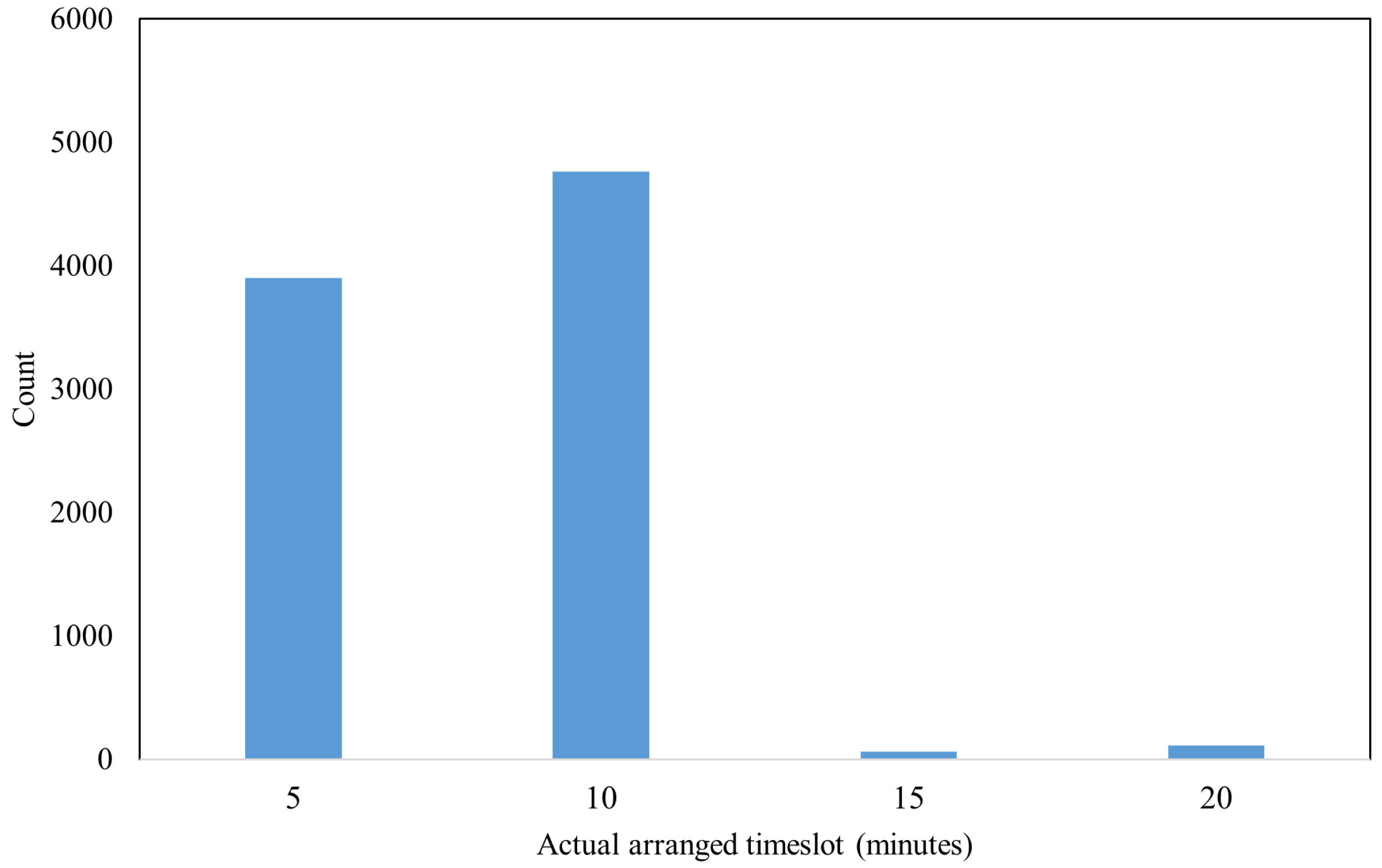
Constraint (7) calculates the adjustment degree of each department’s service time between the first level and second level. The degree of deviation is determined by the absolute distance between the two decisions. Constraints (8) indicate that each department is arranged in one room for one teleconsultation service. Constraints (9) ensure that services are arranged in open teleconsultation rooms. Constraints (10) require the time interval between department services to cope with the uncertainty of the duration of services and the possible future demand. In constraints (10), $\gamma ·\Delta$ represents the size of the time interval. In the case where $\Delta$ takes ten minutes based on the prevalence in practice (see Figure A1 in Appendix A.3), the size of the time interval is determined by $\gamma$. Also, referring to the actual settings, $\gamma$ can be set to three. Constraint (11) mitigates the risk of overtime by restricting the expected end time to be before the off-work hour. Constraint (12) mitigates the risk of overtime by setting the start time to be the on-work hour if the number of waiting demands of departments are larger than or equal to the room expected capacity. These departments will use one room individually.

4. Problem Solving

For solving the proposed model, this section first presents the developed hybrid algorithm, followed by a detailed description of the presorting mechanism for interval constraints.

4.1. The Deep Reinforcement Learning Embedded with Integer Programming

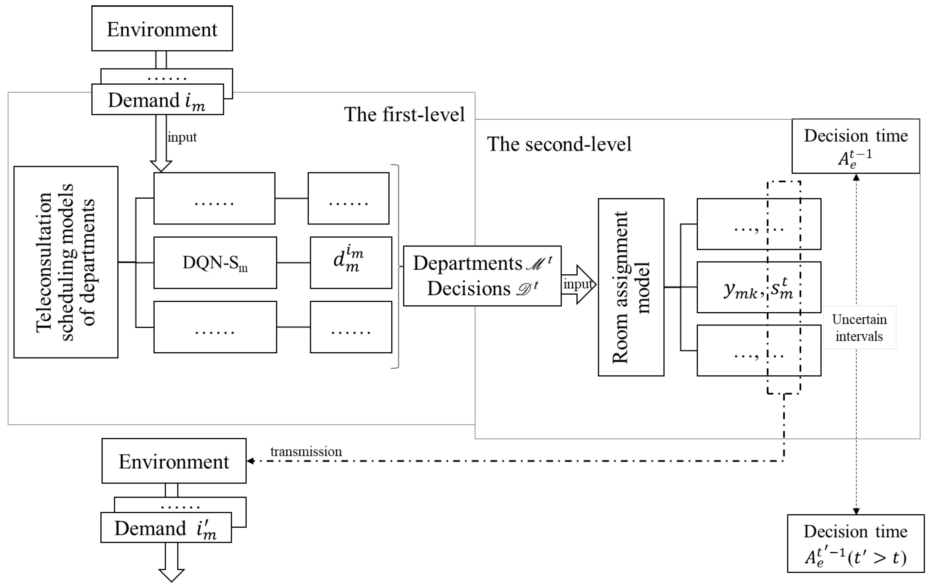
Since the second-level model is constructed based on the results of the first-level model, to solve the two-level model, the first-level model needs to be solved first. The first-level model is solved by the pre-trained DRL algorithm (deep Q-network with a semi-fixed policy, DQN-S). The decision $d_m^{i_m}$ is triggered by the demand $i_m$, which is the first demand in a waiting queue of department m. The second-level model adjusts service time to control overtime risk. If the final service time $s_m^t$ is greatly different from the first-level decision, it can influence the interaction of the DQN-S with the environment. As a result, the second-level model affects the solutions of DQN-S. The process is shown in Figure 2.

Figure 2. Illustration of the solving process of the two-level model.

4.2. The Presorting Mechanism of Interval Constraints

The two-level teleconsultation scheduling model sets time intervals between adjacent department services in the same teleconsultation room to cope with the uncertainty of service duration and potential arrival needs. The time interval setting is achieved using the interval constraint (10). Due to the need to determine the departments where services are arranged in the same room and compare the service start times of these departments pairwise, the interval constraint leads to a large scale of the model in the case of numbers of departments. Therefore, in order to reduce the model size, this study constructs a presorting mechanism for interval constraints to reduce the number of interval constraints.

 Proposition 1. 

Interval constraint presorting proposition.

For departments m and $m^{\prime }$, when the first-level decision $d_m^{i_m}<d_{m^{\prime }}^{i_{m^{\prime }}}$ is made, the second-level decision $s_m^t<s_{m^{\prime }}^t$ can achieve a smaller value compared to $s_m^t>s_{m^{\prime }}^t$ as for the first term, the degree of deviation $\left(g_m+g_{m^{\prime }}\right)$, in the objective (6). Thus, the objective function can achieve a smaller value, obtaining a better scheduling result. The presorting proposition is proved by enumeration analysis as presented in Appendix A.

5. Experimental Results

To validate the proposed model and algorithm, this section conducts teleconsultation scheduling experiments using real-world data and presents a detailed analysis of the results. Specifically, Section 5.1 and Section 5.2 elaborate on the data sources and experimental design, while Section 5.3 showcases the scheduling performance.

5.1. Data

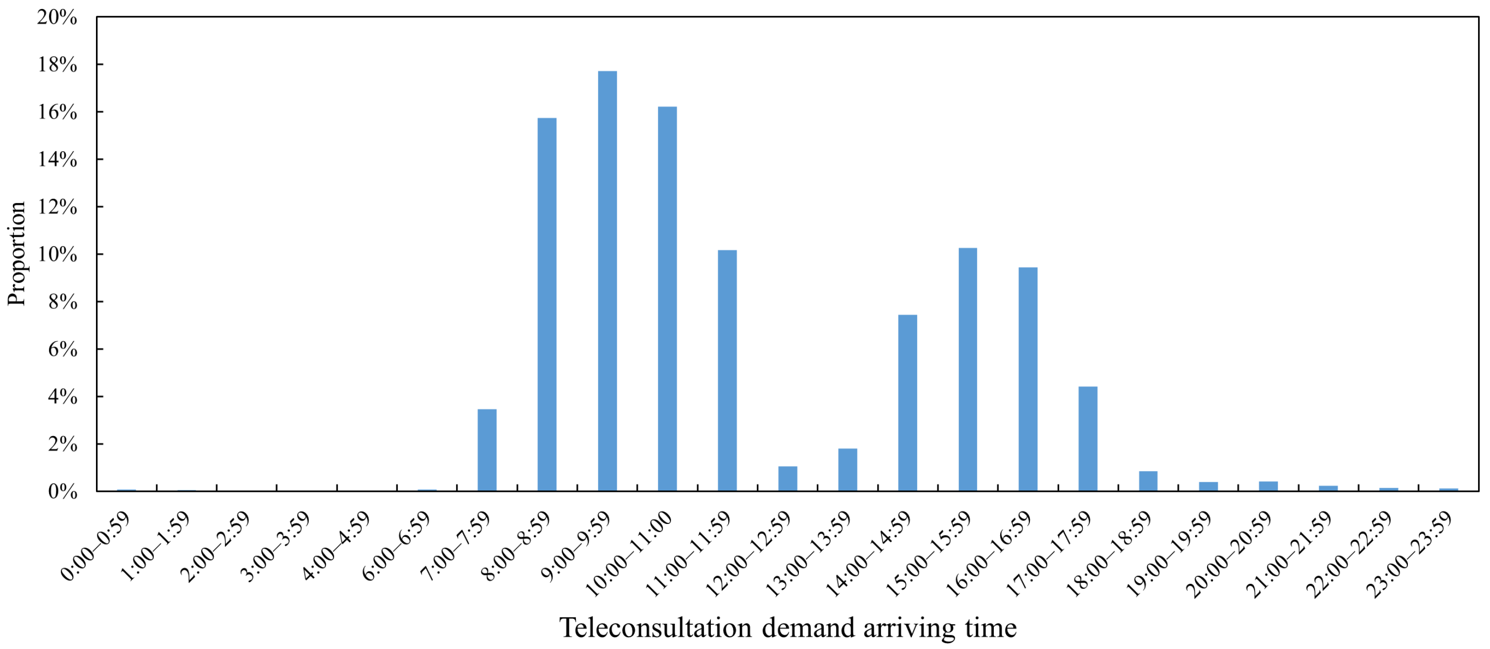
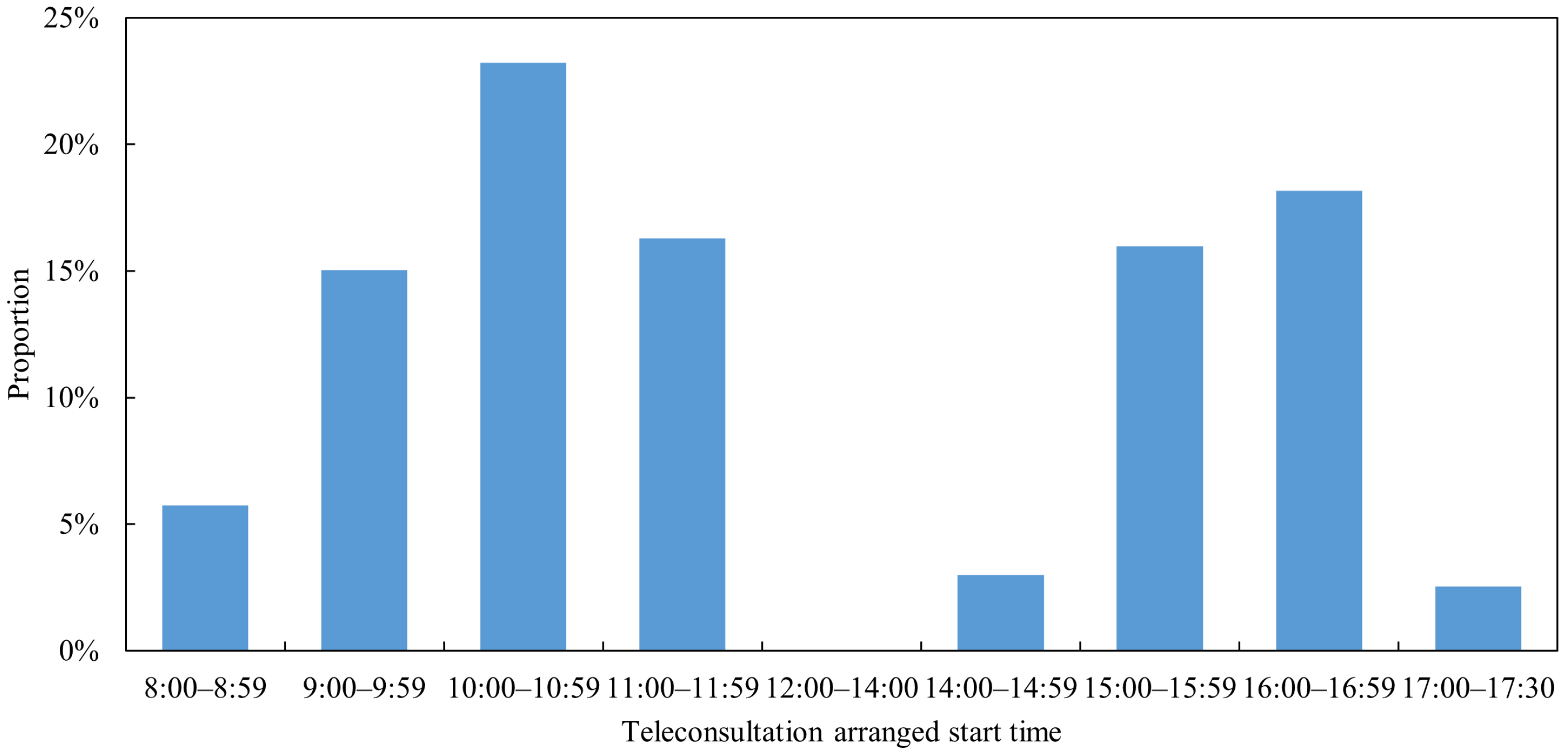
The data utilized in this study are real teleconsultation records, including demand arriving time and service arranged start time provided by the CNTC. A sample of these records is presented in Table A1 (see Appendix A.2). Specifically, demand arrival time is automatically recorded by the system upon submission of a teleconsultation application, and its reliability is guaranteed by the stable operation of the system. In contrast, the scheduled service start time for each department is determined by teleconsultation scheduling staff and documented in the system. Its reliability is validated through the actual teleconsultation services provided. Thus, the data employed in this research are reliable. The daily distributions of the data are displayed in Figure 3 and Figure 4. From the display, it can be seen that most demand arrival time are within the working time of CNTC, as are all arranged teleconsultation start times. At the CNTC, 76 clinical departments offer teleconsultation services. These departments face intermittent teleconsultation demands [33], a key feature characterized by multiple periods of zero demand. Unlike conventional demand, intermittent demand is variable not only in terms of demand volume but also in the intervals between successive demand occurrences. The corresponding teleconsultation service exhibits intermittency equal to or greater than that of the demand, with uncertainties regarding both the start time of teleconsultations and the allocation of teleconsultation rooms.

Figure 3. The daily distribution of demand arrival time.

Figure 4. The daily distribution of arranged teleconsultation start times.

For evaluation purposes, eight departments with relatively high demand volumes were selected as samples. Table 4 presents the demand sizes of these sampled departments over the observation period. The data, collected from 1 January 2018, spans a 60-week period and is divided into three training sets and three testing sets, as detailed in Table A2. The training sets are used to pre-train DQN-S, while the testing sets serve to evaluate scheduling performance.

Table 4. Sample departments for teleconsultation scheduling experiments.

No.	Departments	Total Demand Size	Maximum Daily Demands	Zero Demand Days
1	Respiratory	3101	31	61
2	Neurology	2556	25	64
3	Pediatrics	1777	19	97
4	Orthopedics	1409	21	97
5	Gastroenterology	750	11	144
6	Gynaecology	670	9	155
7	Hepatobiliary and Pancreatic	675	9	141
8	Endocrinology and Metabolic	547	7	174

5.2. Experimental Settings

The first-level model of each department is solved by DQN-S established in the previous study [9]. The DQN-S settings are described below. The input of DQN-S includes the environment variables and the action set. The environmental variables include six date variables and fourteen historical arrival intervals. The six date variables are week; holiday; holiday length; and time information, such as day, hour, and minute. The action set adopts the action set A2 defined in [9].

Based on the output results of DQN-S, Gurobi is used to solve the second-level room allocation model. In the allocation model, the maximum available number of teleconsultation rooms equals the number of departments that require room allocation. The model sets different cost coefficients to analyze the impact of cost coefficients on scheduling performance. The value of the cost coefficient is as follows: $c_1=1,5,10$; $c_2=1,5,10$. For convenience of representation, the cost coefficient is represented in a simplified form; for example, 1-1 represents $c_1=1$, $c_2=1$.

To compare scheduling performance, actual schedules and the schedules of DQN-S are used as benchmarks. The four evaluation criteria used are defined in Table 5. The calculation of room usage distinguishes between the morning and afternoon. The normal service hours in the morning are 8:00∼12:00, and the normal service hours in the afternoon are 14:00∼17:30. When there is a teleconsultation arrangement in a certain teleconsultation room in the morning, the room is used once, and the same applies in the afternoon.

Table 5. The nomenclature used in this paper for performance comparison.

Symbol	Term	Definition (Unit)
DAWT	Demand average waiting time	The average waiting duration before teleconsultation of demands in testing set (hour)
NS	Number of specialist doctor teleconsultations	-
OR	Overtime risk	The potential overtime duration calculated by allocating ten reserved minutes per demand (hour)
RU	Room use	The teleconsultation room usage count

All numerical experiments were coded in Python 3.8 and executed on a PC equipped with an Intel(R) Core(TM) i7-8550U CPU @ 1.80 GHz and 8 GB of RAM. The simulation environment and algorithms were implemented using Python libraries including NumPy, Pandas, DateTime, Math, TensorFlow, and Gurobi.

5.3. Scheduling Performance

5.3.1. The Impact of Cost Coefficients on Scheduling Performance

To investigate the impact of cost coefficients on scheduling performance, the two-level models are built based on three datasets with different cost coefficients for departments 1 (D1) and 2 (D2). The scheduling performance is shown in Table 6.

Table 6. Teleconsultation scheduling performance of departments 1 and 2 on dataset-1.

De.	Performance	Real	Two-Level
			1-1	5-1	10-1	1-5	1-10
D1	DAWT (h)	30.85	18.80	18.81	18.81	18.80	18.80
	NS	18	14	14	14	14	14
	OR (h)	6.70	0.00	0.00	0.00	0.00	0.00
D2	DAWT (h)	24.96	17.82	17.82	17.82	17.82	17.82
	NS	28	15	15	15	15	15
	OR (h)	1.61	0.00	0.00	0.00	0.00	0.00
	RU	42	28	29	29	28	28

From the results in Table 6, two main findings can be obtained. First, the two-level model can improve teleconsultation scheduling effectively. The four performance criteria are decreased by the two-level models. Compared to the actuality, the DAWT of D1 and D2 are reduced by 39% and 29%, respectively. The NS of D1 and D2 are reduced by 22% and 46%. The OR is reduced to zero. And, the RU is reduced by 31% or 33%. Second, changes in cost coefficients have a relatively small impact on the scheduling performance of two-level models. In Table 6, DAWT, NS, and OR of the five models have 0.01 differences in different cost coefficients for D1, and no difference for D2. The RU of two-level models under different cost coefficients are 28 or 29. When the cost of changing start time increases from 1 to 5 and 10, the RU of two-level models show an increasing trend.

To enhance the evaluation, scheduling experiments of D1 and D2 are also conducted on dataset-2 and dataset-3. The results are shown in Table A3 and Table A4 in Appendix A.2, in which findings similar to those in Table 6 can be obtained. In addition, it can be observed from Table A4 that as the cost of opening the room increases, RU decreases. Despite this, changes in the cost coefficient have a relatively small impact on the entire scheduling performance of the two-level model. Therefore, the cost coefficients of 1-1 and 1-5 are used for subsequent experiments on dataset-1.

5.3.2. The Impact of Increasing the Number of Departments on Scheduling Performance

In this section, the number of departments is increased in experiments to analyze the scheduling performance. From the results presented in Table 7, the two-level models maintain their superiority when the number of departments increases to four. Compared to the actuality, DAWT is lowered by 5∼39%, NS by 22∼48%, and RU by 36% and 37%. The total amount of OR declines from 8.58 h to 1.33 h.

Table 7. Teleconsultation scheduling performance with four departments.

Dep.	Performance	Real	Two-Level (1-1)	Two-Level (1-5)
D1	DAWT (h)	30.85	18.84	18.81
	NS	18	14	14
	OR (h)	6.7	0.00	0.00
D2	DAWT (h)	24.96	18.03	18.03
	NS	28	15	15
	OR (h)	1.61	0.00	0.00
D3	DAWT (h)	34.56	23.8	23.8
	NS	19	12	12
	OR (h)	0.26	0.50	0.50
D4	DAWT (h)	24.92	23.46	23.63
	NS	21	11	11
	OR (h)	0.01	0.83	0.83
RU		78	50	49

5.3.3. The Impact of Interval Constraint Presorting Mechanism on Scheduling Performance

In this section, the number of departments is increased to eight analyze the impact of the interval constraint presorting mechanism on scheduling performance. When the number of departments increased to eight, the results in Table 8 not only demonstrate the superior scheduling performance of the two-level model but also prove the effectiveness of the interval constraint presorting mechanism on improving the scheduling. Whether the constraint (10) is presorted or not has no significant impact on the scheduling performance of the two-level model in terms of DAWT, NS, and OR. An important difference is the reduced RU under interval constraint presorting. RU is reduced from 90 and 79 to 78 and 67, respectively. This reduction is explained in Section 6.

Table 8. Teleconsultation scheduling performance with eight departments when the interval constraint presorting mechanism is adopted in the two-level model.

Dep.	Performance	Real	None-Presortin		Presorting
			1-1	1-5	1-1	1-5
D1	DAWT (h)	30.85	18.84	18.84	18.84	18.84
	NS	18	14	14	14	14
	OR (h)	6.7	0.00	0.00	0.00	0.00
D2	DAWT (h)	24.96	18.22	16.74	18.22	18.16
	NS	28	15	16	15	15
	OR (h)	1.61	0.00	0.00	0.00	0.00
D3	DAWT (h)	34.56	23.2	22.02	23.80	23.61
	NS	19	12	12	12	12
	OR (h)	0.26	0.50	0.50	0.50	0.50
D4	DAWT (h)	24.92	23.46	23.49	33.41	24.31
	NS	21	11	11	10	11
	OR (h)	0.01	0.83	0.00	0.00	0.83
D5	DAWT (h)	38.89	21.46	21.40	21.46	22.50
	NS	10	13	13	13	14
	OR (h)	0.00	0.00	0.00	0.00	0.00
D6	DAWT (h)	26.06	19.81	19.53	19.78	18.76
	NS	11	14	15	15	14
	OR (h)	0.00	0.00	0.00	0.00	0.00
D7	DAWT (h)	26.62	21.98	22.02	22.05	21.95
	NS	14	12	12	12	12
	OR (h)	0.02	0.00	0.00	0.00	0.00
D8	DAWT (h)	45.14	19.27	19.19	19.78	19.91
	NS	11	13	13	13	13
	OR (h)	0.00	0.00	0.00	0.00	0.00
RU		95	90	79	78	67

6. Discussion

For discussion, the scheduling performance of the two-level model are first compared with the DQN-S to show its effectiveness on the scheduling optimization. And then, the room usages of departments are analyzed to explain the outperformance of the two-level models on RU reduction. Finally, the amounts of the model constraints are calculated to present the benefit of the presorting mechanism of interval constraints on the two-level model.

6.1. The Comparison of Teleconsultation Scheduling Performance

The scheduling performance of DQN-S is compared to reality to show the necessity of OR controlling in the problem modeling, and two-level models are compared with DQN-S to show the effectiveness of the two-level approach. From the results listed in Table 9, DQN-S can significantly reduce DAWT and NS for departments relative to reality but fail to reduce OR when increasing the number of departments. When there are four and eight departments, the total OR is increased by 7.59 h and by 10.08 h. Therefore, it is necessary to limit OR for teleconsultation scheduling. The two-level approach implements this by the constraints (11) and (12). Given that the DQN-S approach achieves significant reductions in DAWT and NS, the two-level model can further decrease OR and RU. The total OR is decreased to 0 and 1.33 h. The RU is decreased from 86 to 67 when the number of departments is eight. Therefore, the two-level model is effective at improving teleconsultation scheduling.

Table 9. The comparison of teleconsultation scheduling performance between reality, DQN-S, and the two-level model.

The Number of Departments	Performance	Real	DQN-S	Two-Level (1-5, Presorting)
2	Average DAWT (h)	27.91	18.92	18.31
	Average NS	23.00	14.00	14.50
	Total OR (h)	8.31	6.67	0.00
	RU	42	28	28
4	Average DAWT (h)	28.82	21.43	21.07
	Average NS	21.50	12.50	13.00
	Total OR (h)	8.58	16.17	1.33
	RU	78	49	49
8	Average DAWT (h)	31.50	20.83	21.01
	Average NS	16.50	12.88	13.13
	Total OR (h)	8.60	18.68	1.33
	RU	95	86	67

6.2. The Room Usage of Departments

To illustrate how the interval constraint presorting mechanism reduces RU, we analyze the detailed usage of teleconsultation rooms by presenting inter-departmental room-sharing instances of the results of DQN-S and the two-level models. Table 10 shows the instances when the number of departments is eight. Observing the results in Table 10, two conclusions can be drawn. Firstly, in most cases, departments provide teleconsultation services without room sharing during a certain working period. The none-sharing instances account for 80.23% and 52.24%. Secondly, the two-level model with interval constraint presorting reduces RU by increasing room sharing times across departments and the sharing types of departments. There is no case of three departments sharing a room in the results of DQN-S. For the two-level model, the room-sharing instances are 32, and there are six cases where three departments share a room. Therefore, RU is reduced by the two-level model.

Table 10. Comparison of inter-departmental room-sharing instances of DQN-S and the two-level model.

Model	Sharing	D1	D2	D3	D4	D5	D6	D7	D8
DQN-S	None	13	13	8	7	7	7	8	6
	D2D5 *		1			1
	D2D8		1						1
	D3D4			1	1
	D3D6			2			2
	D3D8			1					1
	D4D8				2				2
	D5D6					3	3
	D5D7					2		2
	D5D8					1			1
	D6D7						1	1
	D6D8						1		1
	D7D8							1	1
Two-level	None	11	7	6	3	2	2	2	2
(1-5, presorting)	D1D2D6	1	1				1
	D1D5	1				1
	D1D6	1					1
	D2D3		1	1
	D2D5		2			2
	D2D5D6		1			1	1
	D2D6		2				2
	D2D8		1						1
	D3D5			2		2
	D3D7			1				1
	D3D8			2					2
	D4D5				2	2
	D4D5D8				1	1			1
	D4D6D8				1		1		1
	D4D7				1			1
	D4D7D8				1			1	1
	D4D8				2				2
	D5D6					2	2
	D5D6D7					1	1	1
	D6D7						3	3
	D7D8							3	3

*: D2D5 indicates that department 1 and department 6 shared a consultation room during a certain working period. The other notations follow the same logic.

The room usage is also analyzed between two-level models with different settings. The changes in room opening cost and removing interval constraint presorting influence the usage, as the results show in Table 10 and Table A5. Increasing the opening cost reduces the room usage. When the cost is changed from 1 to 5, RU decreases from 90 to 79 and from 78 to 67. When the opening cost increases to 5, the two-level model outputs more decisions requiring departments to share the teleconsultation room during the same working time period, thus reducing the total RU. This is consistent with the relevant experimental results in Section 5.3.1. In addition, interval constraint presorting can reduce RU. Under the same cost coefficient setting, the two-level model with interval constraint presorting increases both room sharing instances across departments, and the sharing types of departments. When the interval constraint is not presorted, the room-sharing instances are 14 and 27, and there is no case of three departments sharing a room. However, when the interval constraint is presorted, the room-sharing instances increase to 24 and 32, and there are eight cases where three departments share a room. Therefore, by enabling the model to discover more department combinations to share teleconsultation rooms, the interval constraint presorting mechanism can significantly improve the quality of solutions of the two-level model, thus enhancing the model scheduling performance.

6.3. The Changes to the Amount of Model Constraints

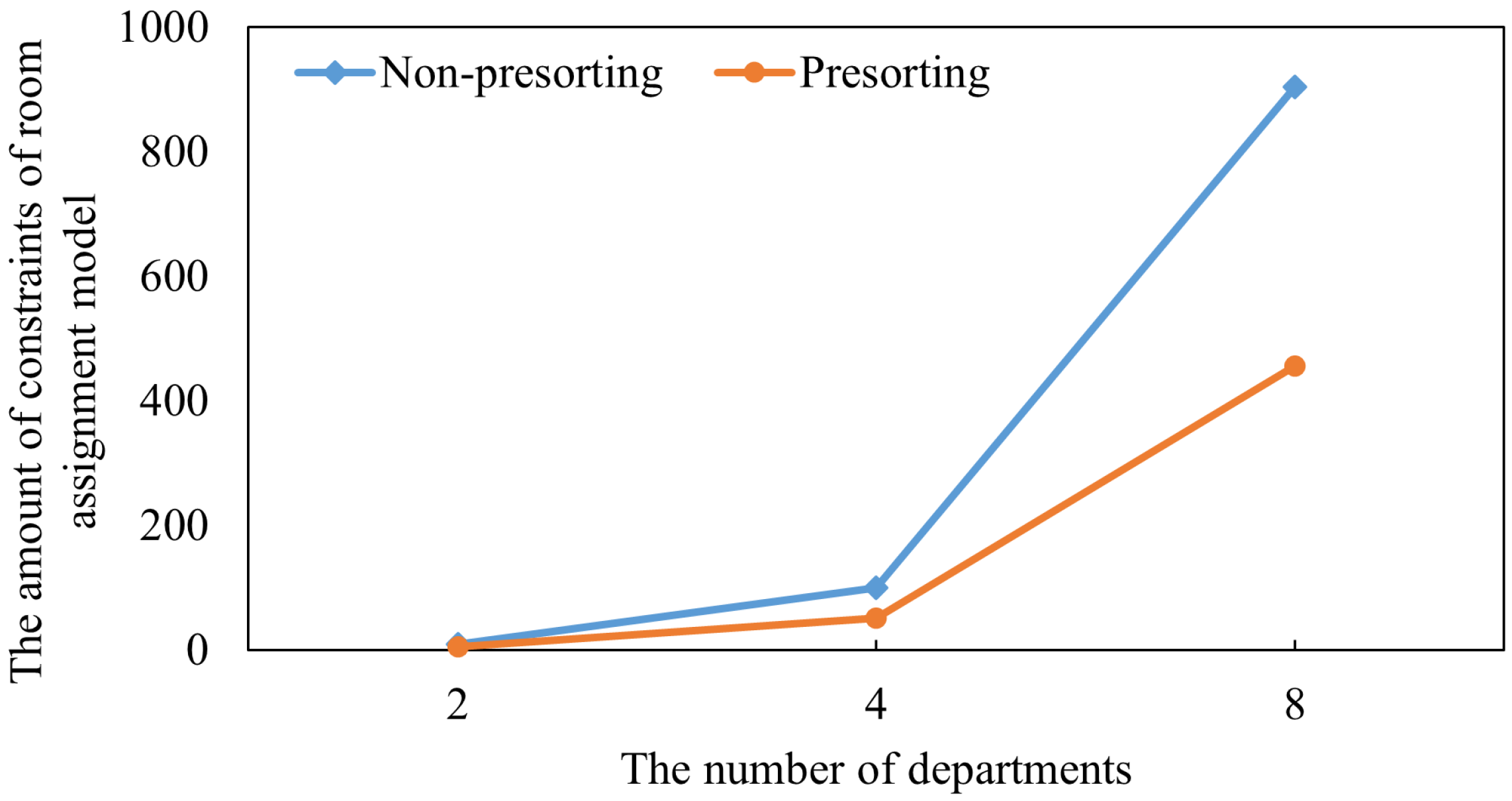
Another benefit from the interval constraint presorting mechanism is the reduced constraint amount of the second-level model. The second-level model is built by using IP to assign rooms. As shown in Figure 5, as the number of departments increases, the number of constraints in the second-level models also increase. When the number of departments increases from 2 to 8 by 4 times, the number of constraints increases from 10 and 6 to 904 and 456, more than 70 times. By presorting the interval constraints, the number of model constraints is almost half of that when not presorting. When the number of constraints is significantly reduced, model solving can be accelerated.

Figure 5. The changes in the constraint amount of the second-level model with department amount.

7. Conclusions

In this paper, teleconsultation scheduling is further optimized by prioritizing the optimization of service frequency and incorporating downstream room utilization and overtime risk as considerations. For this purpose, a two-level approach is proposed based on a data-driven dynamic teleconsultation scheduling model. Based on the optimized start time in the first-level models to optimize service frequency, second-level models are built to allocate teleconsultation room and adjust the start time to reduce overtime risk. The frequency is optimized for service sustainability due to demand intermittency. The generally applicable environment of this study has the characteristic of intermittent demand and the target of control event frequency. For other analogous environments or problems, such as the purchase of spare parts, the proposed methods can be used with appropriate adjustments.

To solve the two-level model, an embedding DRL and IP solver method is constructed. And, to improve the solutions, an interval constraint presorting mechanism is developed. Based on actual teleconsultation data, numerical experiments verify the effectiveness of the proposed scheduling model, the solving method, and the presorting mechanism. There are three main conclusions.

• In different experimental settings, two-level models can maintain their effectiveness in improving teleconsultation scheduling performance. When the cost coefficients are changed and the number of departments is increased, two-level models can outperform reality. The DAWT can be lowered by 5.86∼57.49% and NS by 14.29∼52.38%.
• The two-level model further improves teleconsultation scheduling by reducing OR. Compared to reality, DQN-S can significantly reduce DAWT and NS for a single department but increase OR. Compared to DQN-S, the two-level model can significantly reduce OR by 0.17∼4.67 h, without losing the outperformance in DAWT and NS.
• The two-level model also improves teleconsultation scheduling by reducing RU by 22.09∼37.18%. There are two effective approaches to lowering RU: one is increasing the opening cost in the two-level model, and the other is implementing the interval constraint presorting mechanism. When interval constraints are presorted, the number of department combinations for sharing teleconsultation rooms can be increased by 5 and 10. In the results of the two-level models, there are eight cases where three departments share a room.

While this study has made progress in teleconsultation scheduling, it has certain limitations that warrant further refinement in future research. From the perspective of modeling, the proposed teleconsultation scheduling model does not consider the uncertainties of service duration and no-show behavior, due to data limitation. This work can be extended by addressing such uncertainties either through theoretical simulation analysis or the collection of additional supporting data. Furthermore, incorporating emergency priority represents a valuable direction for extension. From the perspective of model solving, this study solves the first-level model based on a basic DRL algorithm. There are many other DRL algorithms and techniques that can be tested in future studies.

Appendix A.1. Proof for the Presorting Mechanism of Interval Constraints

 Proof of Proposition 1. 

The proposition is proved as follows.

Constraint (7) indicates $\left(g_m+g_{m^{\prime }}\right)\ge 0$. When $\left(g_m+g_{m^{\prime }}\right)=0$, if and only if $s_m^t=d_m^{i_m}<d_{m^{\prime }}^{i_{m^{\prime }}}=s_{m^{\prime }}^t$, the proposition is established.

When $\left(g_m+g_{m^{\prime }}\right)>0$, let the gap of the first decisions be $u_0$, that is, $d_m^{i_m}=d_{m^{\prime }}^{i_{m^{\prime }}}-u_0$. There are two cases for the second decisions. When $s_m^t<s_{m^{\prime }}^t$, let $s_m^t=s_{m^{\prime }}^t-u_1$; when $s_m^t>s_{m^{\prime }}^t$, let $s_m^t=s_{m^{\prime }}^t+u_2$. The proposition is proved in the following four situations.

• When $d_m^{i_m}<s_m^t$ and $d_{m^{\prime }}^{i_{m^{\prime }}}<s_{m^{\prime }}^t$, the deviation is calculated using Equation (A1) when $s_m^t<s_{m^{\prime }}^t$ and Equation (A2) when $s_m^t>s_{m^{\prime }}^t$. Compared with the right items in the equations, it can be drawn that Equation (A1) < Equation (A2). Thus, the proposition is proved.

  $$\begin{array}{cc}\hfill & g_m+g_{m^{\prime }}=\left(s_m^t-d_m^{i_m}\right)+\left(s_{m^{\prime }}^t-d_{m^{\prime }}^{i_{m^{\prime }}}\right)=2·s_{m^{\prime }}^t-2·d_{m^{\prime }}^{i_{m^{\prime }}}-u_1+u_0,\hfill \\ \hfill & d_m^{i_m}<s_m^t<s_{m^{\prime }}^t,d_m^{i_m}<d_{m^{\prime }}^{i_{m^{\prime }}}<s_{m^{\prime }}^t.\hfill \end{array}$$

  (A1)

  $$\begin{array}{cc}\hfill & g_m+g_{m^{\prime }}=\left(s_m^t-d_m^{i_m}\right)+\left(s_{m^{\prime }}^t-d_{m^{\prime }}^{i_{m^{\prime }}}\right)=2·s_{m^{\prime }}^t-2·d_{m^{\prime }}^{i_{m^{\prime }}}+u_2+u_0,\hfill \\ \hfill & d_m^{i_m}<d_{m^{\prime }}^{i_{m^{\prime }}}<s_{m^{\prime }}^t<s_m^t.\hfill \end{array}$$

  (A2)
• When $d_m^{i_m}<s_m^t$ and $d_{m^{\prime }}^{i_{m^{\prime }}}>s_{m^{\prime }}^t$, the deviation is calculated using Equation (A3) when $s_m^t<s_{m^{\prime }}^t$ and Equation(A4) when $s_m^t>s_{m^{\prime }}^t$. Compared with the right items in the equations, it can be drawn that Equation (A3) < Equation (A4). Thus, the proposition is proved.

  $$\begin{array}{cc}\hfill & g_m+g_{m^{\prime }}=\left(s_m^t-d_m^{i_m}\right)+\left(d_{m^{\prime }}^{i_{m^{\prime }}}-s_{m^{\prime }}^t\right)=-u_1+u_0,\hfill \\ & d_m^{i_m}<s_m^t<s_{m^{\prime }}^t<d_{m^{\prime }}^{i_{m^{\prime }}}.\hfill \end{array}$$

  (A3)

  $$g_m+g_{m^{\prime }}=\left(s_m^t-d_m^{i_m}\right)+\left(d_{m^{\prime }}^{i_{m^{\prime }}}-s_{m^{\prime }}^t\right)=u_2+u_0.$$

  (A4)
• When $d_m^{i_m}>s_m^t$ and $d_{m^{\prime }}^{i_{m^{\prime }}}<s_{m^{\prime }}^t$, the deviation is calculated using Equation (A5) when $s_m^t<s_{m^{\prime }}^t$. When $s_m^t>s_{m^{\prime }}^t$, there is $d_m^{i_m}>s_m^t>s_{m^{\prime }}^t>d_{m^{\prime }}^{i_{m^{\prime }}}$, which contradicts the proposition setting, $d_m^{i_m}<d_{m^{\prime }}^{i_{m^{\prime }}}$. Therefore, this condition is removed. When $s_m^t<s_{m^{\prime }}^t$, the deviation can be calculated and the proposition is established.

  $$g_m+g_{m^{\prime }}=\left(d_m^{i_m}-s_m^t\right)+\left(s_{m^{\prime }}^t-d_{m^{\prime }}^{i_{m^{\prime }}}\right)=u_1-u_0,s_m^t<d_m^{i_m}<d_{m^{\prime }}^{i_{m^{\prime }}}<s_{m^{\prime }}^t.$$

  (A5)
• When $d_m^{i_m}>s_m^t$ and $d_{m^{\prime }}^{i_{m^{\prime }}}>s_{m^{\prime }}^t$, the deviation is calculated using Equation (A6) when $s_m^t<s_{m^{\prime }}^t$ and Equation (A7) when $s_m^t>s_{m^{\prime }}^t$. Compared with the right items in the equations, it can be drawn that Equation (A6) < Equation (A7). Thus, the proposition is proved.

  $$\begin{array}{cc}\hfill & g_m+g_{m^{\prime }}=\left(d_m^{i_m}-s_m^t\right)+\left(s_{m^{\prime }}^t-d_{m^{\prime }}^{i_{m^{\prime }}}\right)=2d_m^{i_m}-2s_m^t-u_1+u_0,\hfill \\ \hfill & s_m^t<d_m^{i_m}<d_{m^{\prime }}^{i_{m^{\prime }}},s_m^t<s_{m^{\prime }}^t<d_{m^{\prime }}^{i_{m^{\prime }}}.\hfill \end{array}$$

  (A6)

  $$\begin{array}{cc}\hfill & g_m+g_{m^{\prime }}=\left(d_m^{i_m}-s_m^t\right)+\left(s_{m^{\prime }}^t-d_{m^{\prime }}^{i_{m^{\prime }}}\right)=2d_m^{i_m}-2s_m^t+u_1+u_0,\hfill \\ \hfill & s_{m^{\prime }}^t<s_m^t<d_m^{i_m}<d_{m^{\prime }}^{i_{m^{\prime }}}.\hfill \end{array}$$

  (A7)

  Based on the above proof, the interval constraint presorting proposition holds. □

Appendix A.2. Tables

Table A1. Samples of used teleconsultation records.

Clinical Departments	Demand Arrival Time	Service Arranged Start Time (in Ascending Order)
Orthopedics	2 January 2018 08:33	2 January 2018 11:00
Neurology	2 January 2018 08:33	2 January 2018 11:00
Neurology	2 January 2018 08:36	2 January 2018 11:10
Neurology	2 January 2018 09:03	2 January 2018 11:20
Respiratory	2 January 2018 08:54	2 January 2018 15:20
Respiratory	2 January 2018 08:33	2 January 2018 15:30
Respiratory	1 January 2018 08:17	2 January 2018 15:40
Respiratory	2 January 2018 09:39	2 January 2018 15:45
Respiratory	2 January 2018 10:16	2 January 2018 15:50
Respiratory	2 January 2018 11:01	2 January 2018 15:55
Respiratory	2 January 2018 10:37	2 January 2018 16:00
Respiratory	2 January 2018 10:17	2 January 2018 16:05
Neurology	2 January 2018 10:34	2 January 2018 16:00
Neurology	2 January 2018 10:09	2 January 2018 16:10
Neurology	2 January 2018 10:17	2 January 2018 16:20
Neurology	2 January 2018 10:18	3 January 2018 15:00
Neurology	2 January 2018 11:12	3 January 2018 15:10
Neurology	2 January 2018 11:46	3 January 2018 15:20

Table A1. Samples of used teleconsultation records.

Clinical Departments	Demand Arrival Time	Service Arranged Start Time (in Ascending Order)
Orthopedics	2 January 2018 08:33	2 January 2018 11:00
Neurology	2 January 2018 08:33	2 January 2018 11:00
Neurology	2 January 2018 08:36	2 January 2018 11:10
Neurology	2 January 2018 09:03	2 January 2018 11:20
Respiratory	2 January 2018 08:54	2 January 2018 15:20
Respiratory	2 January 2018 08:33	2 January 2018 15:30
Respiratory	1 January 2018 08:17	2 January 2018 15:40
Respiratory	2 January 2018 09:39	2 January 2018 15:45
Respiratory	2 January 2018 10:16	2 January 2018 15:50
Respiratory	2 January 2018 11:01	2 January 2018 15:55
Respiratory	2 January 2018 10:37	2 January 2018 16:00
Respiratory	2 January 2018 10:17	2 January 2018 16:05
Neurology	2 January 2018 10:34	2 January 2018 16:00
Neurology	2 January 2018 10:09	2 January 2018 16:10
Neurology	2 January 2018 10:17	2 January 2018 16:20
Neurology	2 January 2018 10:18	3 January 2018 15:00
Neurology	2 January 2018 11:12	3 January 2018 15:10
Neurology	2 January 2018 11:46	3 January 2018 15:20

Table A2. Subsets of data for teleconsultation scheduling experiments.

Data Division	Dataset-1	Dataset-2	Dataset-3
Training sets	1∼16 weeks	21∼36 weeks	41∼56 weeks
Testing sets	17∼20 weeks	37∼40 weeks	57∼60 weeks

Table A2. Subsets of data for teleconsultation scheduling experiments.

Data Division	Dataset-1	Dataset-2	Dataset-3
Training sets	1∼16 weeks	21∼36 weeks	41∼56 weeks
Testing sets	17∼20 weeks	37∼40 weeks	57∼60 weeks

Table A3. Teleconsultation scheduling performance of departments 1 and 2 on dataset-2.

De.	Performance	Real	Two-Level
			1-1	5-1	10-1	1-5	1-10
D1	DAWT (h)	33.19	19.11	19.11	19.11	19.11	19.11
	NS	15	14	14	14	14	14
	OR (h)	4.17	0	0	0	0	0
D2	DAWT (h)	26.25	17.24	17.37	17.37	17.24	17.24
	NS	15	14	15	15	14	14
	OR (h)	3.61	0	0	0	0	0
	RU	26	25	27	27	25	25

Table A3. Teleconsultation scheduling performance of departments 1 and 2 on dataset-2.

De.	Performance	Real	Two-Level
			1-1	5-1	10-1	1-5	1-10
D1	DAWT (h)	33.19	19.11	19.11	19.11	19.11	19.11
	NS	15	14	14	14	14	14
	OR (h)	4.17	0	0	0	0	0
D2	DAWT (h)	26.25	17.24	17.37	17.37	17.24	17.24
	NS	15	14	15	15	14	14
	OR (h)	3.61	0	0	0	0	0
	RU	26	25	27	27	25	25

Table A4. Teleconsultation scheduling performance of departments 1 and 2 on dataset-3.

De.	Performance	Real	Two-Level
			1-1	5-1	10-1	1-5	1-10
D1	DAWT (h)	32.03	15.09	15.09	15.09	15.09	15.09
	NS	14	11	11	11	11	11
	OR (h)	10.89	0.17	0.17	0.17	0.17	0.17
D2	DAWT (h)	23.39	15.26	15.26	15.26	15.26	15.26
	NS	19	16	16	16	16	16
	OR (h)	0.51	0.17	0.17	0.17	0.17	0.17
	RU	27	25	25	26	25	25

Table A4. Teleconsultation scheduling performance of departments 1 and 2 on dataset-3.

De.	Performance	Real	Two-Level
			1-1	5-1	10-1	1-5	1-10
D1	DAWT (h)	32.03	15.09	15.09	15.09	15.09	15.09
	NS	14	11	11	11	11	11
	OR (h)	10.89	0.17	0.17	0.17	0.17	0.17
D2	DAWT (h)	23.39	15.26	15.26	15.26	15.26	15.26
	NS	19	16	16	16	16	16
	OR (h)	0.51	0.17	0.17	0.17	0.17	0.17
	RU	27	25	25	26	25	25

Table A5. Comparison of inter-departmental room-sharing instances for two-level models under different interval constraint presorting and room opening cost configurations.

Interval Constraint Presorting	Room Opening Cost	RU	Sharing	D1	D2	D3	D4	D5	D6	D7	D8
No	1	90	None	12	11	9	11	10	8	8	7
			D1D6	2					2
			D2D5		1			1
			D2D6		1				1
			D2D8		2						2
			D3D5			1		1
			D3D8			2					2
			D5D6					1	1
			D6D7						2	2
			D7D8							2	2
No	5	79	None	11	6	7	7	7	5	4	5
			D1D2	1	1
			D1D5	1				1
			D1D6	1					1
			D2D5		1			1
			D2D6		5				5
			D2D8		3						3
			D3D5			1		1
			D3D7			2				2
			D3D8			2					2
			D4D5				1	1
			D4D7				1			1
			D4D8				2				2
			D5D6					1	1
			D5D7					1		1
			D6D7						3	3
			D7D8							1	1
Yes	1	78	None	11	10	9	5	6	4	2	7
			D1D5D7	1				1		1
			D1D6	2					2
			D2D3		1	1
			D2D5		2			2
			D2D6		1				1
			D2D8		1						1
			D3D5			1		1
			D3D8			1					1
			D4D5				1	1
			D4D6				1		1
			D4D7				2			2
			D4D8				1				1
			D5D6					2	2
			D6D7						4	4
			D6D7D8						1	1	1
			D7D8							2	2

Table A5. Comparison of inter-departmental room-sharing instances for two-level models under different interval constraint presorting and room opening cost configurations.

Interval Constraint Presorting	Room Opening Cost	RU	Sharing	D1	D2	D3	D4	D5	D6	D7	D8
No	1	90	None	12	11	9	11	10	8	8	7
			D1D6	2					2
			D2D5		1			1
			D2D6		1				1
			D2D8		2						2
			D3D5			1		1
			D3D8			2					2
			D5D6					1	1
			D6D7						2	2
			D7D8							2	2
No	5	79	None	11	6	7	7	7	5	4	5
			D1D2	1	1
			D1D5	1				1
			D1D6	1					1
			D2D5		1			1
			D2D6		5				5
			D2D8		3						3
			D3D5			1		1
			D3D7			2				2
			D3D8			2					2
			D4D5				1	1
			D4D7				1			1
			D4D8				2				2
			D5D6					1	1
			D5D7					1		1
			D6D7						3	3
			D7D8							1	1
Yes	1	78	None	11	10	9	5	6	4	2	7
			D1D5D7	1				1		1
			D1D6	2					2
			D2D3		1	1
			D2D5		2			2
			D2D6		1				1
			D2D8		1						1
			D3D5			1		1
			D3D8			1					1
			D4D5				1	1
			D4D6				1		1
			D4D7				2			2
			D4D8				1				1
			D5D6					2	2
			D6D7						4	4
			D6D7D8						1	1	1
			D7D8							2	2

Appendix A.3. Figure

Figure A1. The distribution of arranged teleconsultation timeslots during the observed window.

Figure A1. The distribution of arranged teleconsultation timeslots during the observed window.

References

1. Sood, S.; Mbarika, V.; Jugoo, S.; Dookhy, R.; Doarn, C.R.; Prakash, N.; Merrell, R.C. What Is Telemedicine? A Collection of 104 Peer-reviewed Perspectives and Theoretical Underpinnings. Telemed. J. e-Health 2007, 13, 573–590. [Google Scholar] [CrossRef] [PubMed]
2. Lamas, C.d.A.; Alves, P.G.S.; de Araujo, L.N.; Paes, A.B.d.S.; Cielo, A.C.; Lopes, L.M.d.A.; de Melo, A.L.A.; Yokoyama, T.; Savastano, C.P.; Scudeller, P.G.; et al. Telehealth Initiative to Enhance Primary Care Access in Brazil (UBS plus Digital Project): Multicenter Prospective Study. J. Med. Internet Res. 2025, 27, e68434. [Google Scholar] [CrossRef]
3. Cui, F.; Ma, Q.; He, X.; Zhai, Y.; Wang, Z. Implementation and Application of Telemedicine in China: Cross-Sectional Study. JMIR MHealth UHealth 2020, 8, e18426. [Google Scholar] [CrossRef] [PubMed]
4. Zhai, Y.; Jia, Q.; Yan, Q.; Jie, Z. Duration Predictionof Teleconsultation Services Based on the ATT-FC-LSTM Model. Chin. J. Manag. 2025, 22, 568–576. [Google Scholar] [CrossRef]
5. Ji, M.; Wang, S.; Peng, C.; Li, J. Two-stage robust telemedicine assignment problem with uncertain service duration and no-show behaviours. Comput. Ind. Eng. 2022, 169, 108226. [Google Scholar] [CrossRef]
6. Qiao, Y.; Ran, L.; Li, J. Optimization of Teleconsultation Using Discrete-Event Simulation from a Data-Driven Perspective. Telemed. e-Health 2019, 26, 1114–1125. [Google Scholar] [CrossRef]
7. Qiao, Y.; Ran, L.; Li, J.L.; Zhai, Y.K. Design and Comparison of Scheduling Strategy for Teleconsultation. Technol. Health Care 2021, 29, 939–953. [Google Scholar] [CrossRef] [PubMed]
8. Wan, M.; Shukla, N.; Li, J.; Pradhan, B. Optimization of teleconsultation appointment scheduling in National Telemedicine Center of China. Comput. Ind. Eng. 2023, 183, 109492. [Google Scholar] [CrossRef]
9. Chen, W.; Li, J. Teleconsultation dynamic scheduling with a deep reinforcement learning approach. Artif. Intell. Med. 2024, 149, 102806. [Google Scholar] [CrossRef]
10. Qiao, Y.; Zhai, Y.; Ma, R.; Ji, M.; Lu, W. Optimizing teleconsultation scheduling to make healthcare greener. J. Clean. Prod. 2023, 422, 138569. [Google Scholar] [CrossRef]
11. Jiang, Y.p.; Zhang, Y.; Gao, Z.; Zheng, T.W. Logic-based Benders decomposition for doctor-patient matching and scheduling considering chronic patients’ online consultation time preference. Comput. Oper. Res. 2025, 183, 107207. [Google Scholar] [CrossRef]
12. Huang, J.; Morrice, D.; Bard, J. Coordinated scheduling for in-clinic and virtual medicine patients in a multi-station network. IISE Trans. 2024, 56, 437–457. [Google Scholar] [CrossRef]
13. Cai, Y.; Song, H.; Wang, S. Managing appointment-based services with electronic visits. Eur. J. Oper. Res. 2024, 315, 863–878. [Google Scholar] [CrossRef]
14. Guo, H.; Xie, Y.; Jiang, B.; Tang, J. When outpatient appointment meets online consultation: A joint scheduling optimization framework. Omega-Int. J. Manag. Sci. 2024, 127, 103101. [Google Scholar] [CrossRef]
15. Erdogan, S.A.; Krupski, T.L.; Lobo, J.M. Optimization of Telemedicine Appointments in Rural Areas. Serv. Sci. 2018, 10, 261–276. [Google Scholar] [CrossRef]
16. Guo, H.; Xie, Y.; Yu, D.; Jiang, B. Outpatient appointment scheduling optimization considering online further consultation demand. Syst. Eng. Theory Pract. 2021, 42, 3279–3293. [Google Scholar]
17. Chen, W.; Chen, L.; Shen, X.; Zhang, Y.; Wang, X. Appointment scheduling considering outpatient unpunctuality under telemedicine services. Mathematics 2025, 13, 2591. [Google Scholar] [CrossRef]
18. Ji, M.; Mosaffa, M.; Ardestani-Jaafari, A.; Li, J.; Peng, C. Integration of text-mining and telemedicine appointment optimization. Ann. Oper. Res. 2023, 341, 621–645. [Google Scholar] [CrossRef]
19. Qiao, Y.; Ran, L.; Li, J.L.; Wang, Z. Research on Teleconsultation Appointment Scheduling Problem Based on Two-stage Stochastic Programming. Chin. J. Manag. Sci. 2024, 32, 86–93. [Google Scholar] [CrossRef]
20. Wang, J.; Guo, H.; Tsui, K.L. Two-stage robust optimisation for surgery scheduling considering surgeon collaboration. Int. J. Prod. Res. 2021, 59, 6437–6450. [Google Scholar] [CrossRef]
21. Azaiez, M.N.; Gharbi, A.; Kacem, I.; Makhlouf, Y.; Masmoudi, M. Two-stage no-wait hybrid flow shop with inter-stage flexibility for operating room scheduling. Comput. Ind. Eng. 2022, 168, 108040. [Google Scholar] [CrossRef]
22. Li, N.; Chen, H.; Pei, Z.; Wang, T. Jointly Appointment Scheduling in a Two-Phase Service System with Two Types of Patients Considering Multiple Servers and Stochastic Service Time. IEEE Trans. Autom. Sci. Eng. 2024, 22, 1339–1352. [Google Scholar] [CrossRef]
23. Çelik, B.; Gul, S.; Karsu, Ö. Maintaining fairness in stochastic chemotherapy scheduling. Omega 2025, 137, 103338. [Google Scholar] [CrossRef]
24. Zhang, J.; Dridi, M.; El Moudni, A. A two-phase optimization model combining Markov decision process and stochastic programming for advance surgery scheduling. Comput. Ind. Eng. 2021, 160, 107548. [Google Scholar] [CrossRef]
25. Zhang, L.; Zhang, Y.; Bai, Q. Two-stage medical supply chain scheduling with an assignable common due window and shelf life. J. Comb. Optim. 2019, 37, 319–329. [Google Scholar] [CrossRef]
26. Dong, Y.; Zheng, W.; Ma, Z.; He, Z. Two-stage robust optimization for public health emergency project scheduling with uncertain activity durations. Comput. Oper. Res. 2025, 182, 107135. [Google Scholar] [CrossRef]
27. Guo, J.; Pozehl, W.; Cohn, A. A two-stage partial fixing approach for solving the residency block scheduling problem. Health Care Manag. Sci. 2023, 26, 363–393. [Google Scholar] [CrossRef] [PubMed]
28. Isakov, A.; Peregorodiev, D.; Tomilov, I.; Ye, C.; Gusarova, N.; Vatian, A.; Boukhanovsky, A. Real-Time Scheduling with Independent Evaluators: Explainable Multi-Agent Approach. Technologies 2024, 12, 259. [Google Scholar] [CrossRef]
29. El-Shenhabi, A.N.; Abdelhay, E.H.; Mohamed, M.A.; Moawad, I.F. A Reinforcement Learning-Based Dynamic Clustering of Sleep Scheduling Algorithm (RLDCSSA-CDG) for Compressive Data Gathering in Wireless Sensor Networks. Technologies 2025, 13, 25. [Google Scholar] [CrossRef]
30. Zhao, Z.; Lee, C.K.M.; Ren, J. A two-level charging scheduling method for public electric vehicle charging stations considering heterogeneous demand and nonlinear charging profile. Appl. Energy 2024, 355, 122278. [Google Scholar] [CrossRef]
31. Xu, K.; Ye, C.; Gong, H.; Sun, W. Reinforcement Learning-Based Multi-Objective of Two-Stage Blocking Hybrid Flow Shop Scheduling Problem. Processes 2024, 12, 51. [Google Scholar] [CrossRef]
32. Jabeur, M.H.; Mahjoub, S.; Toublanc, C.; Cariou, V. Optimizing integrated lot sizing and production scheduling in flexible flow line systems with energy scheme: A two level approach based on reinforcement learning. Comput. Ind. Eng. 2024, 190, 110095. [Google Scholar] [CrossRef]
33. Chen, W.; Li, J. Teleconsultation Demand Classification and Service Analysis. BMC Med. Inform. Decis. Mak. 2021, 21, 245. [Google Scholar] [CrossRef] [PubMed]