Deep Learning-Based Aerodynamic Analysis for Diverse Aircraft Configurations

Abstract

In this study, a neural network was developed to predict the aerodynamic characteristics of fixed-wing aircraft with two lifting surfaces of various aerodynamic configurations. The proposed neural network model can incorporate 23 parameters to describe the aerodynamic configuration of an aircraft. A methodology for discrete geometric parameterization of aerodynamic configurations is introduced, enabling coverage of various combinations of relative positions of aircraft components. This study presents an approach to database construction and automated sample generation for neural network training. Furthermore, a procedure is provided for data preprocessing and correlation analysis of the input variables. The optimization process of the hyperparameters of the multilayer perceptron (MLP) architecture is described. The neural network models are validated through comparison with numerical simulations. Finally, several aerodynamic design problems are addressed, and the key advantages of the developed MLP-based surrogate aerodynamic models are demonstrated.

1. Introduction

The accuracy and efficiency of calculating the aerodynamic characteristics of an aircraft are critical in the early design stages. At present, the problem of aerodynamic design of aircraft is typically formalized in terms of nonlinear mathematical programming (NLP) [1,2,3] and is defined as the search for a vector of design variables x = {x₁, x₂, …, x_n}, which minimizes the objective function F(x) within the feasible area Ω:

$$\begin{gathered} \left|F\left({\mathit{x}}^{\mathit{o}\mathit{p}\mathit{t}}\right)\right|\le \left|F\left(\mathit{x}\right)\right| \forall \mathit{x}\in \mathsf{\Omega }, \\ \mathsf{\Omega }=\left\{\mathit{x}: q\left(\mathit{x}\right)<0\right\} \end{gathered}$$

(1)

The accuracy of the design result depends on the fidelity of the mathematical models used for the direct evaluation of the objective function and constraints, the degree of parameterization of the models, and the number of variables being considered.

In recent decades, significant progress has been achieved in the field of numerical methods for aerohydrodynamics and multiphysics processes of engineering systems, enabling high-fidelity simulations that account for a high level of geometric detail of the studied objects. In such cases, gas flows are described by the Navier–Stokes equations supplemented with various models and algorithms of different levels of complexity, depending on the problem formulation [4]. Simultaneously, the early stages of design require the consideration of several technical solutions: the number of design variables may be in the order of 10¹ to 10² or more. The exploration of many variables inevitably encounters the rapid growth of problem dimensionality and the associated sharp increase in computational costs under time constraints. Under such conditions, the use of high-fidelity numerical models becomes impractical, since the computation of a single combination of design variables may take several hours, while the required number of evaluations for aerodynamic layout optimization with as few as 10 parameters may reach 10⁴ or more, depending on the algorithm. Other areas of aeronautical science face similar difficulties in employing resource-intensive models, such as real-time flight dynamics simulation, robust optimization, and generative design.

In the practice of aerodynamic computations, there also exist computationally in-expensive numerical models, such as the lattice Boltzmann method [5], which makes it possible to obtain responses to changes in aircraft configuration parameters in real time. However, such methods have significant applicability limitations, particularly with respect to the range of Reynolds and Mach numbers.

Recently, neural network-based models (surrogate models) [6,7] have gained significant popularity in aerodynamic computations of aircraft, owing to their very high computational efficiency. The performance of neural network models exceeds that of even the simplest numerical methods by one to two orders of magnitude, which opens new opportunities for solving aerodynamic optimization problems at the early stages of aircraft design by enabling the consideration of a substantially larger number of design variable combinations within shorter computational times.

Most existing studies on the application of artificial neural networks (ANNs) in aerodynamics have primarily focused on predicting the characteristics of two-dimensional airfoils [8,9,10,11,12,13,14,15] or, less frequently, isolated lifting surfaces of an aircraft [16,17,18], which limits their applicability to the entire aircraft. These studies provide useful insights into the aerodynamics of airfoils and isolated wings but cannot capture the interactions between multiple lifting surfaces and other aircraft components. The authors [19] used ANN to select wing profiles to optimize the design of aircraft-type unmanned aerial vehicles. The approaches presented in [20,21] considered the use of neural network models for computing the aerodynamic characteristics of a complete airframe; however, they accounted for only two input parameters (angle of attack and Mach number) and a single output parameter. Similarly, refs. [22,23] also employed a limited number of input and output parameters, thereby restricting their ability to address different aircraft types. This limitation constrains the capability of the models in [20,21] across a broader range of design parameters and flight conditions. Moreover, in many existing works, neural network architectures were often predefined without systematic hyperparameter optimization, typically employing a fixed number of hidden layers and neurons [8,9]. In several cases, only a single hidden layer was used [20], which may be insufficient for accurately capturing complex aerodynamic relationships, even at the preliminary design stage. Despite the potential advantages of using different activation functions in different layers, most existing studies have relied on the same activation function across all hidden layers [8,18,24]. Although the possibility of employing multiple activation functions has been explored [24], the parameter of search space has not been sufficiently investigated.

One of the advantages of surrogate models is their ability to populate the database with characteristics obtained through computational methods, experimental techniques, or a combination of both, depending on the specific task. For example, previous studies [25,26] presented results on the estimation of fuel consumption for transport aircraft at the design stage using deep-learning-based MLP, trained on fuel consumption data from currently operating aircraft across different flight phases.

In [27], a neural network-based model was developed to determine the aerodynamic characteristics of transport-category aircraft. A database of various aircraft geometries and their corresponding aerodynamic characteristics was generated through numerical mathematical modeling of potential flows, supplemented with a viscosity correction, to train the neural network. The resulting neural network was proposed for use in the parametric optimization of transport aircraft configurations at the early design stages.

A review of most existing studies on the application of neural networks for the prediction of aerodynamic coefficients reveals that the potential for comprehensive parameterization of aerodynamic configurations has largely been overlooked. Most of these studies have narrowly focused on the selection of a limited set of parameters within a specific, predefined aerodynamic layout, rather than addressing the broader challenge of generalizable configuration parameterization.

In this context, the present study seeks to extend the capabilities of aerodynamic surrogate modeling, building upon the groundwork established in [18], by enabling discrete geometric parameterization of complete aircraft aerodynamic configurations and evaluating a broader spectrum of integral aerodynamic characteristics while explicitly accounting for prescribed margins of longitudinal static stability. The proposed enhancement of surrogate modeling is achieved by sequentially optimizing neural network hyperparameters using evolutionary algorithms. The successful implementation of such neural network models is expected to open new opportunities for optimization studies in the early stages of aircraft design: the substantial acceleration of computational performance will allow for the exploration of a significantly larger set of design variable combinations, thereby improving the overall accuracy and efficiency of the aircraft design process.

The objective of this study is to enhance the computational efficiency of predicting the aerodynamic characteristics of aircraft-type configurations with varying aerodynamic layouts by employing neural networks.

2. Materials and Methods

2.1. Problem Formulation

The proposed methodology is based on low-speed aircraft-type configurations featuring different aerodynamic configurations with two lifting surfaces. The surrogate models developed in this study are performed using MLP, which has been widely employed in related works due to its capability to capture complex nonlinear dependencies inherent in aircraft aerodynamics.

The generation of the MLP is based on specialized databases. These databases contain combinations of the geometric parameters of the aircraft configuration of interest together with the corresponding aerodynamic characteristics. The geometric parameters and aerodynamic conditions such as angle of attack and flight velocity, are considered as the input parameters, while the associated aerodynamic coefficients serve as the output parameters for the trainable perceptron. Each parameter combination in the database, which effectively represents a specific aerodynamic configuration with its corresponding aerodynamic characteristics, is hereafter referred to as an individual. The neural network model for aerodynamic coefficient prediction obtained through deep learning can be formally expressed as: f: X → Y, where $\mathit{X}\subset {\mathbb{R}}^n$ (geometric characteristics and flight conditions) and $\mathit{Y}\subset {\mathbb{R}}^m$ (aerodynamic coefficients).

Figure 1 presents the block scheme methodology.

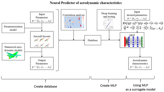
Figure 1. Algorithm of neural predictor.

2.2. Geometric Parameterization of Aircraft Configurations

The configuration of each individual in the database is defined by a set of input design variables (23). These variables are divided into geometric parameters (20 variables) and flight conditions (3 variables). Table 1 and Table 2 present the ranges of the input variables considered in this study.

Table 1. Geometric design variables.

	Variables	Min	Max
1	Aspect ratio of the forward wing AR1	4.0	15.0
2	Sweep of the forward wing Λ1, [°]	0.0	45.0
3	Taper of the forward wing λ1	1.0	3.0
4	Installation angle of the forward wing δ1, [°]	0.0	5.0
5	Aspect ratio of the aftward wing AR2	4.0	15.0
6	Sweep of the aftward wing Λ2, [°]	−45.0	45.0
7	Taper of the aftward wing λ2	1.0	3.0
8	Installation angle of the aftward wing δ2, [°]	−5.0	5.0
9	Relative distance between two wings ${\overline{L}}_2$	2.0	6.0
10	Relative area ${\overline{S}}_2$	0.1	0.9
11	Aspect ratio of the vertical tail AR3	2.0	4.0
12	Relative area of the vertical tail ${\overline{S}}_3$	0.05	0.3
13	Twist angle of the main wing φ, [°]	−5.0	0.0
14	Dihedral angle of the main wing ψ, [°]	0.0	10.0
15	Type of fuselage configuration nF	0	1
16	Type of horizontal tail configuration nHT	0	1
17	Dihedral angle of horizontal tail ψ2, [°]	30.0	50.0
18	Relative position of the horizontal tail zHT	0	1
19	Reference area SΣ, [m2]	1.0	50.0
20	Longitudinal static stability margin $\Delta$	−0.3	0.0

Table 2. Flight conditions.

	Variables	Min	Max
1	Flight speed V, [m/s]	20	90
2	Angle of attack α, [°]	−10.0	10.0
3	Flight altitude H, [m]	0	10,000

The quantities presented in Table 1 are calculated using the following formulas: ${\overline{S}}_2={\displaystyle \raisebox{1ex}{$S_2$}\!\left/ \!\raisebox{-1ex}{$S_1$}\right.}$, $S_{\Sigma }=S_1+S_2$, ${\overline{S}}_3={\displaystyle \raisebox{1ex}{$S_3$}\!\left/ \!\raisebox{-1ex}{$\left(S_1+S_2\right)$}\right.}$, where $S_1$, $S_2$, $S_3$ denote the absolute areas of the front lifting surface, the rear lifting surface, and the vertical tail, respectively. The main lifting surface is defined as the one with the larger area. The longitudinal static stability margin Δ is determined as the relative distance between the pitching moment reference point and the aerodynamic focus.

Some parameters from Table 1 are shown graphically in Figure 2.

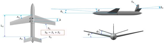
Figure 2. Illustration of geometric parameters.

A distinctive feature of this study is the ability to simultaneously consider a wide range of aerodynamic configurations based on different possible combinations of fuselage types (single-fuselage (Figure 3a–c,j); twin-boom (Figure 3d–f,k); twin-fuselage (Figure 3g–i,l)) and tail configurations (conventional tail (Figure 3a,d,g); V-tail (Figure 3b,e,h); inverted V-tail (Figure 3c,f,i)), along with the ratio of the rear to front wing areas (conventional, tandem, or canard configurations) (Figure 3). The position of the horizontal tail is considered at three locations—root, mid-span, and tip of the vertical tail—through the design variable 0 < z_HT < 1 (Figure 3). Thus, the relative position of the horizontal tail with respect to the vertical tail is defined as follows: root section 0 ≤ z_HT ≤ 1/3; mid-span 1/3 < z_HT < 2/3; tip section 2/3 ≤ z_HT. The type of fuselage configuration is parameterized by the variable n_F: twin-fuselage 0 ≤ n_F ≤ 1/3; single-fuselage 1/3 < n_F < 2/3; twin-boom 2/3 ≤ n_F. Similarly, the type of horizontal tail configuration is defined through the parameter n_HT: conventional tail 0 ≤ n_HT ≤ 1/3; V-tail 1/3 < n_HT < 2/3; inverted V-tail 2/3 ≤ n_HT.

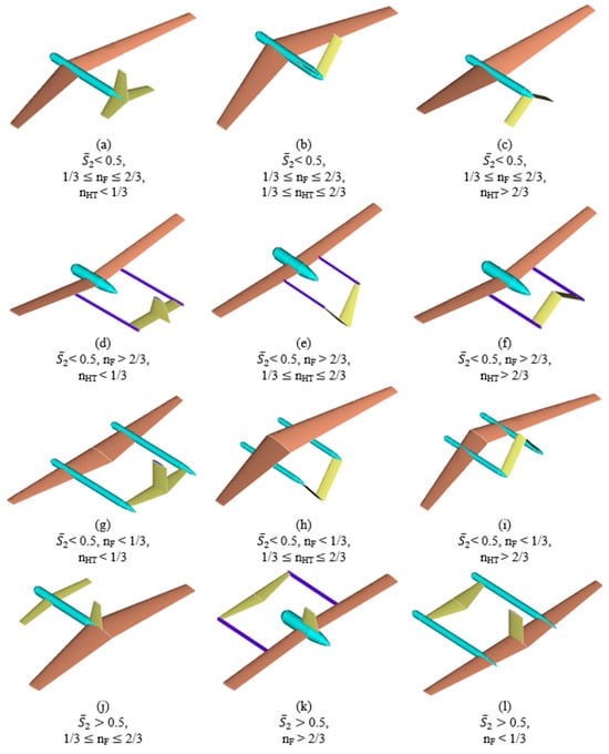
Figure 3. Illustration of possible aircraft configurations with different parameters. (a) $\overline{S_2}<0.5,$1/3 < nF < 2/3, nHT < 1/3; (b) $\overline{S_2}<0.5,$1/3 < nF < 2/3, nHT < 2/3; (c) $\overline{S_2}<0.5,$1/3 < nF < 2/3, nHT > 2/3; (d) $\overline{S_2}<0.5,$nF > 2/3, nHT < 1/3; (e)$\overline{S_2}<0.5,$nF > 2/3, 1/3 ≤ nHT ≤ 2/3; (f) $\overline{S_2}<0.5,$nF > 2/3, nHT > 2/3; (g) $\overline{S_2}<0.5,$nF < 1/3, nHT < 1/3; (h) $\overline{S_2}<0.5,$nF < 1/3, 1/3 ≤ nHT < 2/3; (i) $\overline{S_2}<0.5,$nF < 1/3, nHT > 2/3; (j) $\overline{S_2}>0.5,$1/3 ≤ nF ≤ 2/3; (k) $\overline{S_2}>0.5,$nF > 2/3; (l) $\overline{S_2}>0.5,$nF < 1/3.

2.3. Determination of Aerodynamic Characteristics and Training Dataset Generation

The open-source Python-based software OpenVSP 3.45.3 [28] was used to construct the aerodynamic characteristics database. OpenVSP is based on the vortex lattice method (VLM), which uses a vortex representation of thin lifting surfaces. This method is particularly well suited for modeling subsonic, inviscid, and incompressible flows. It provides an effective balance between computational speed and accuracy when determining aircraft aerodynamic characteristics in the early stages of design.

According to the theoretical foundations of VLM [29,30], the midsurface of the lifting plane is modeled by a system of vortex frames (Figure 4a), each of which contains a П-shaped vortex consisting of an attached vortex and two free ones. The circulation intensity of each vortex is calculated based on solving systems of linear equations A·Γ = V_n, where A is the aerodynamic influence matrix (determined by the geometry of the lifting plane), Γ is the desired column matrix of circulations, and V_n is the column matrix of normal velocities obtained from the non-permeability condition of the lifting surface. Based on the calculation of the distribution of circulations Γ over the lifting surface, the distribution of lifting force over the lifting surface is calculated. The induced drag is calculated based on the distribution of induced velocities and the downwash flow in the Trefftz plane. Figure 4b shows a vortex model of aerodynamics for an arbitrary layout in the OpenVSP software.

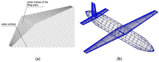
Figure 4. A vortex model (a) of thin lifting surface; (b) of an aircraft layout in OpenVSP 3.45.3 software.

The database of individuals’ geometric characteristics was populated using the Latin Hypercube Sampling (LHS) method [31,32]. This approach generated 28,000 combinations (individuals) through randomized sampling of the 23 parameters listed in Table 1 and Table 2.

The output parameters to be determined (seven in total) include the lift coefficient (C_L), drag coefficient (C_D), pitching moment coefficient (C_M), the derivative of the rolling moment coefficient with respect to sideslip angle ($C_l^{\beta }$), the derivative of the yawing moment coefficient with respect to sideslip angle ($C_n^{\beta }$), the derivative of the pitching moment coefficient with respect to the lift coefficient ($C_m^{C_L}$), and the pitching moment damping coefficient ($C_m^{{\omega }_y}$). OpenVSP was employed in batch mode using a custom Python control script. This enabled automated batch processing of large datasets, automated parameterization of aerodynamic configurations of individuals, as well as parallel computations to accelerate the database generation process. By integrating the OpenVSP API with Python, 3.13.5 a streamlined methodology was developed for the rapid generation of geometrical models, their subsequent aerodynamic evaluation, and storage in the database (Table 3).

Table 3. Structure of the database for training the direct model.

Inputs	x1	Aspect ratio of the forward wing AR1
	x2	Sweep of the forward wing Λ1, [°]
	x3	Taper of the forward wing λ1
	x4	Installation angle of the forward wing δ1, [°]
	x5	Aspect ratio of the aftward wing AR2
	x6	Sweep of the aftward wing Λ2, [°]
	x7	Taper of the aftward wing λ1
	x8	Installation angle of the aftward wing δ2, [°]
	x9	Relative distance between two wings ${\overline{L}}_2$
	x10	Relative area ${\overline{S}}_2$
	x11	Aspect ratio of the vertical tail AR3
	x12	Relative area of the vertical tail ${\overline{S}}_3$
	x13	Twist angle of the main wing φ, [°]
	x14	Dihedral angle of the main wing ψ, [°]
	x15	Type of fuselage configuration nF
	x16	Type of horizontal tail configuration nHT
	x17	Dihedral angle of horizontal tail ψ2, [°]
	x18	Relative position of the horizontal tail zHT
	x19	Flight speed V, [m/s]
	x20	Angle of attack α, [°]
	x21	Reference area SΣ, [m2]
	x22	Longitudinal static stability margin $\mathsf{\Delta }$
	x23	Flight altitude H, [m]
Outputs	y1	Drag coefficient CD
	y2	Lift coefficient CL
	y3	Pitching moment coefficient Cm
	y4	Derivative of rolling moment with respect to sideslip angle $C_l^{\beta }$
	y5	Derivative of yawing moment with respect to sideslip angle $C_n^{\beta }$
	y6	Derivative of pitching moment with respect to lift $C_m^{C_L}$
	y7	Pitch damping $C_m^{{\omega }_y}$

2.4. Data Quality Assessment and Correlation Analysis

The accuracy of the neural network model strongly depends on the quality of the data in the training samples. To ensure the reliability of the input data, several stages of preliminary data preprocessing were carried out:

-

To prevent overfitting and to enhance the generalization capability of the model, the data in the sample were randomly shuffled;

-

From the initial dataset consisting of 28,000 individuals, 849 cases with unsuccessful combinations of geometric parameters leading to poor aerodynamic characteristics were excluded, leaving a database with 27,151 individuals. Figure 5 presents the frequency distribution histograms of aerodynamic characteristics across individuals after this filtering step;

-

Normalization of both input and output variables to the range [0, 1] was performed using the min–max scaling method.

$$x_{norm}={\displaystyle \frac{x-x_{min}}{x-x_{max}}},$$

(2)

where x_min and x_max denote the minimum and maximum values of the corresponding parameter within the dataset.

Figure 5. Distribution histograms of aerodynamic characteristics: (a) C_D; (b) C_L; (c) C_m; (d) $C_l^{\beta }$; (e) $C_n^{\beta }$; (f) $C_m^{C_L}$; (g) $C_m^{{\omega }_y}$.

This procedure ensures a uniform scale across all parameters, thereby eliminating differences in dimensionality. Such normalization improves the convergence of neural network hyperparameter optimization algorithms and contributes to more stable model performance in subsequent applications.

-

A strong correlation between the input and output data must ensure the accurate training of the neural network. This is particularly important for the inverse model in which the input variables are selected to achieve the prescribed output characteristics. The Spearman’s correlation coefficient [33,34] was employed for the dataset correlation analysis, which is defined as follows:

$$\rho \left({\tilde{X}}_i,{\tilde{Y}}_i\right)={\displaystyle \frac{{\sum }_{i=1}^n\left(R_i-\overline{R}\right)\left(S_i-\overline{S}\right)}{\sqrt{{\sum }_{i=1}^n{\left(R_i-\overline{R}\right)}^2}\sqrt{{\sum }_{i=1}^n{\left(S_i-\overline{S}\right)}^2}}}$$

(3)

where R_i = rank(${\tilde{X}}_i$); S_i = rank(${\tilde{Y}}_i$); $\overline{R}$—the mean rank of R_i; $\overline{S}$—the mean rank of S_i.

The value of Spearman’s correlation coefficient ρ ranges from −1 to +1, where values close to ±1 indicate a strong monotonic correlation (positive or negative), while values close to 0 indicate a weak or no relationship.

The correlation analysis is applied to identify the variables that exert the greatest influence on the corresponding outputs. Figure 6 presents the results of this analysis, visualized in the form of a color-coded matrix, where the color intensity reflects the magnitude of the coefficient correlation, and the numerical values are displayed inside the cells.

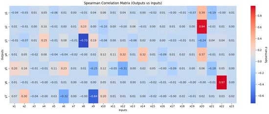
Figure 6. Spearman’s correlation matrix for the direct problem.

The correlations between the input parameters and aerodynamic characteristics obtained using Spearman’s coefficient demonstrate overall consistency with the fundamental laws of aerodynamics. The correlation structure reflects physically justified trends, such as the influence of geometric and flight regime parameters on the forces and moments generated in the flow. The absence of contradictions with theoretical expectations indicates the correctness of the employed model and the initial data’s reliability. Thus, the identified relationships confirm that the computational model adequately captures the aircraft’s aerodynamic behavior within the investigated parameter range.

2.5. Selection of Multilayer Perceptron Hyperparameters

The MLP was implemented using the Keras 3.0 library. The MLP architecture was selected through sequential evolutionary optimization of hyperparameters, including: the number of hidden layers (1–6); the number of neurons per layer; types of activation functions (ReLU, LeakyReLU, ELU, Sigmoid); batch size; and the number of folds in K-fold cross-validation.

During the training of the MLP, the Mean Squared Error (MSE) was employed as the loss function, while the Adam optimizer (Adaptive Moment Estimation) with a learning rate of 0.001 was used. The model performance was evaluated using two key metrics: the Root Mean Squared Error (RMSE), which reflects the average prediction error, and the coefficient of determination (R²), which characterizes the proportion of explained variance in the output data.

To enable proper integration into the genetic representation of individuals, activation functions were encoded as integers (1–4). Each hidden layer was allowed to employ its own activation function.

The early stopping method was applied to prevent overfitting: training was terminated when no improvement in validation error was observed. The number of epochs was limited to 1000.

The optimal type of activation function and the number of neurons per layer were jointly selected using the Differential Evolution algorithm to reduce computational costs, while the remaining hyperparameters were optimized separately in a sequential manner.

For the training stage, 82% of the individuals from the database were considered, while the remaining 18% were left for the testing stage.

Table 4, Table 5, Table 6, Table 7 and Table 8 present the results of the training stage, which include the selection of hidden layers, neurons, activation functions, K-Fold values, and batch size. In Table 4, Table 7 and Table 8, the optimal architectures that were used further are highlighted in green.

Table 4. Selection of the number of hidden layers.

MLP Architechture	MSE	RMSE	R2
			CD	CL	CM	${\mathit{C}}_{\mathit{l}}^{\mathit{\beta }}$	${\mathit{C}}_{\mathit{n}}^{\mathit{\beta }}$	${\mathit{C}}_{\mathit{m}}^{{\mathit{C}}_{\mathit{L}}}$	${\mathit{C}}_{\mathit{m}}^{{\mathit{\omega }}_{\mathit{y}}}$
23-64-7	0.0025	0.0499	0.946	0.987	0.642	0.584	0.871	0.926	0.932
23-64-64-7	0.0018	0.0428	0.960	0.992	0.781	0.647	0.895	0.929	0.961
23-64-64-64-7	0.0017	0.0405	0.961	0.993	0.841	0.667	0.904	0.927	0.966
23-64-64-64-64-7	0.0017	0.0410	0.965	0.993	0.820	0.667	0.908	0.926	0.960
23-64-64-64-64-64-7	0.0018	0.0425	0.960	0.992	0.814	0.655	0.900	0.924	0.962

Table 5. Selection of the number of neurons per hidden layer.

MLP Architecture	MSE	RMSE	R2
			CD	CL	CM	${\mathit{C}}_{\mathit{l}}^{\mathit{\beta }}$	${\mathit{C}}_{\mathit{n}}^{\mathit{\beta }}$	${\mathit{C}}_{\mathit{m}}^{{\mathit{C}}_{\mathit{L}}}$	${\mathit{C}}_{\mathit{m}}^{{\mathit{\omega }}_{\mathit{y}}}$
23-512-435-370-7	0.0010	0.0285	0.975	0.993	0.896	0.805	0.935	0.955	0.977

Table 6. Selection of the activation function.

HL1	HL2	HL3
LEAKY_RELU	LEAKY_RELU	SIGMOID

Table 7. Selection of the k value in K-Fold cross-validation.

k	MSE	RMSE	R2
			CD	CL	CM	${\mathit{C}}_{\mathit{l}}^{\mathit{\beta }}$	${\mathit{C}}_{\mathit{n}}^{\mathit{\beta }}$	${\mathit{C}}_{\mathit{m}}^{{\mathit{C}}_{\mathit{L}}}$	${\mathit{C}}_{\mathit{m}}^{{\mathit{\omega }}_{\mathit{y}}}$
5	0.0010	0.0185	0.9749	0.9933	0.8958	0.8053	0.9345	0.9546	0.9767
8	0.0007	0.0254	0.9802	0.9938	0.9298	0.8689	0.9506	0.9665	0.9819
10	0.0006	0.0228	0.9840	0.9946	0.9412	0.8950	0.9614	0.9721	0.9845
12	0.0006	0.0230	0.9835	0.9942	0.9424	0.8975	0.9602	0.9756	0.9835
14	0.0005	0.0203	0.9858	0.9942	0.9543	0.9229	0.9674	0.9790	0.9873
16	0.0005	0.0217	0.9837	0.9943	0.9502	0.9074	0.9631	0.9777	0.9851
18	0.0005	0.0205	0.9848	0.9941	0.9568	0.9249	0.9661	0.9789	0.9878

Table 8. Selection of batch size.

Batch Size	MSE	RMSE	R2
			CD	CL	CM	${\mathit{C}}_{\mathit{l}}^{\mathit{\beta }}$	${\mathit{C}}_{\mathit{n}}^{\mathit{\beta }}$	${\mathit{C}}_{\mathit{m}}^{{\mathit{C}}_{\mathit{L}}}$	${\mathit{C}}_{\mathit{m}}^{{\mathit{\omega }}_{\mathit{y}}}$
15	0.0010	0.0185	0.9749	0.9933	0.8958	0.8053	0.9345	0.9546	0.9767
20	0.0005	0.0203	0.9858	0.9942	0.9543	0.9229	0.9674	0.9790	0.9873
25	0.0005	0.0193	0.9871	0.9958	0.9549	0.9192	0.9701	0.9813	0.9867
30	0.0004	0.0173	0.9890	0.9969	0.9592	0.9308	0.9737	0.9840	0.9886
35	0.0004	0.0183	0.9873	0.9958	0.9575	0.9221	0.9700	0.9815	0.9890

2.5.1. Selection of the Number of Hidden Layers in Architecture

The analysis results demonstrate that increasing the number of hidden layers from 1 to 3 leads to a significant decrease in MSE from 0.0025 to 0.0017, while RMSE is reduced from 0.0499 to 0.0405, indicating a notable reduction in the mean squared prediction error. However, a further increase in the number of layers to 4 and 5 does not yield additional error reduction; on the contrary, it results in a slight increase (MSE rises to 0.0017 and 0.0018), which indicates the effect of overfitting.

When considering the coefficient of determination (R²) for individual aerodynamic characteristics, the architecture with three hidden layers (23-64-64-64-7) demonstrates the most balanced and highest performance. In particular, the R² for the lift coefficient C_L reaches a very high value of ~0.993, indicating an almost perfect prediction for this characteristic. The R² for the drag coefficient C_D is ~0.961, which is slightly lower compared to C_L and reflects a more complex nonlinear dependency. For the pitching moment C_M, the lowest R² value of ~0.8409 is observed, which is associated with the high sensitivity and complexity of modeling this parameter.

Increasing the number of hidden layers to 4 and 5 provides only a marginal improvement in R² for certain characteristics, while leading to a decrease or fluctuations in R² for others, such as C_M and C_L. This confirms the conclusion that, for the available training dataset, the architecture with three hidden layers already provides sufficient approximation of the nonlinear relationships between input and output variables while maintaining generalization capability.

2.5.2. Selection of the Number of Neurons per Hidden Layer and the Activation Function

In the next stage of the study, an integer-based differential evolution algorithm was employed to further improve the accuracy of aerodynamic characteristic prediction. The objective was to optimize not only the number of neurons in each hidden layer but also to select individual activation functions for each network layer.

As a result of the optimization, an architecture with three hidden layers (23-512-435-370-7) was obtained, with LEAKY_RELU selected as the activation function for the first and second layers and SIGMOID for the third hidden layer. This architecture provided a noticeable improvement in prediction accuracy compared with the previously considered architectures.

The MSE value decreased to 0.0010 and the RMSE to 0.0285 (Table 5), which is almost twice as good as the previous best result obtained with the 23-64-64-64-7 architecture (MSE ~0.0017, RMSE ~0.0405) (Table 4). It is particularly important to note the substantial increase in the coefficients of determination (R²) for individual aerodynamic characteristics.

This improvement can be explained by the fact that the increased number of neurons enables the network to model more complex nonlinear relationships between the input parameters and the aerodynamic characteristics. At the same time, the appropriate selection of activation functions ensures both high sensitivity of the model to weak signals (due to LEAKY_RELU) and the ability to capture saturated nonlinear dependencies and boundaries (using SIGMOID in the last hidden layer) (Table 6).

Thus, the use of an integer-based differential evolution algorithm made it possible to not only automate the hyperparameter tuning process but also identify an architecture that demonstrates significantly better performance across all key metrics. The resulting network combines high accuracy (low MSE and RMSE) with improved generalization capability (high R² values), making it a more reliable tool for predicting the complex object aerodynamic characteristics.

2.5.3. Selection of the K-Fold Cross-Validation Value

In the process of selecting the optimal value of k for the K-Fold cross-validation method applied to the MLP with 23 input variables, three hidden layers, and seven outputs for predicting aerodynamic characteristics, the results presented in Table 7 demonstrate a trend of improved model performance as k increases from 5 to 18.

Increasing the number of folds in the K-Fold method results in the model being tested on progressively smaller portions of the dataset at each training step, while being trained on larger subsets. This reduces error variance and enhances the reliability of assessing the model’s generalization capability. In the present case, as k increases from 5 to 14, the RMSE and R² indicators show a steady and consistent improvement, indicating the model’s ability to robustly extract aerodynamic patterns from different data subsets. The component-wise metrics also stabilize, with reduced fluctuations, further confirming the improvement in model robustness. However, at k = 18, further gains in accuracy become marginal compared to k = 14, suggesting saturation. Moreover, the increased computational cost makes the use of excessively large k values impractical. Therefore, k = 14 is not only optimal in terms of accuracy but also balanced with respect to computational efficiency for the considered aerodynamic task.

2.5.4. Selection of Batch Size in Architecture

The optimal MLP architecture with 23 input parameters, three hidden layers, and seven output characteristics achieved high prediction accuracy with a batch size of 30. The mean squared error was 0.0004, and the RMSE value was 0.0173, indicating a minimal deviation between the predicted and reference values. The coefficients of determination for most output parameters exceeded 0.98, reaching 0.9969 for the lift coefficient, 0.9890 for the drag coefficient, and 0.9886 for the pitch damping (Table 8). High R² values were also recorded for the pitching moment and its derivative with respect to the lift coefficient, highlighting the model’s ability to reproduce stable aerodynamic relationships, including those with pronounced nonlinear features.

The process of selecting the optimal hyperparameter values for the MLP architecture was carried out on a personal computer equipped with an Intel(R) Core(TM) i7-6700 CPU 3.40 GHz and 64 GB of RAM. The entire process took 92,156 s (25.6 h).

As a result of the optimization process, the MLP architecture presented in Table 9 was obtained, while the corresponding evaluation metrics are summarized in Table 10.

Table 9. MLP hyperparameters for the direct problem.

Hyperparameter			Value
Number of hidden layers			3
Number of neurons in each hidden layer	Layer No.	1	512
		2	435
		3	370
Activation function	Layer No.	1	LEAKY_RELU
		2	LEAKY_RELU
		3	SIGMOID
Number of folds in K-Fold cross-validation			14
Batch size			30

Table 10. Evaluation metrics of the MLP for the direct problem (training stage).

MSE	RMSE	R2
		CD	CL	CM	${\mathit{C}}_{\mathit{l}}^{\mathit{\beta }}$	${\mathit{C}}_{\mathit{n}}^{\mathit{\beta }}$	${\mathit{C}}_{\mathit{m}}^{{\mathit{C}}_{\mathit{L}}}$	${\mathit{C}}_{\mathit{m}}^{{\mathit{\omega }}_{\mathit{y}}}$
0.00035	0.01607	0.9986	0.9991	0.9975	0.9982	0.9973	0.9988	0.9991

As a result of training the MLP neural network architecture, high values of the determination coefficient R² were obtained for individual aerodynamic characteristics: R² = 0.9987 for C_D, R² = 0.999 for C_L, R² = 0.9975 for C_M, as well as other indicators at the levels of 0.9981, 0.9972, 0.9988, and 0.9991. These statistical results demonstrate the successful training of the neural network in capturing complex nonlinear dependencies between the input parameters and aerodynamic characteristics. The developed direct model can reproduce more than 96–99% of the data variance.

3. Results and Analysis

3.1. Testing of the Surrogate Model

Figure 7 shows the R² results corresponding to the testing stage. The R² results for the aerodynamic coefficients C_L, C_D, and C_M are like those obtained with other architectures dedicated to predicting aerodynamic coefficients and considering high-dimensionality problems (R² values ~0.99). Table 11 compares the proposed MLP architecture and 3 other architectures.

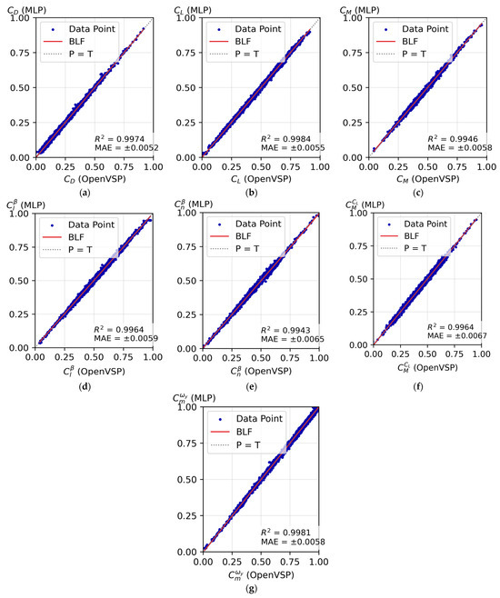
Figure 7. Regression analysis of the final MLP architecture at the testing stage: (a) drag coefficient C_D; (b) lift coefficient C_L; (c) pitching moment C_M; (d) derivative of rolling moment with respect to sideslip angle $C_l^{\beta }$; (e) derivative of yawing moment with respect to sideslip angle $C_n^{\beta }$; (f) derivative of pitching moment with respect to lift $C_m^{C_L}$; (g) pitch damping $C_m^{{\omega }_y}$.

Table 11. Performance analysis of the prediction of the aerodynamic coefficients for airplanes of different neural networks.

Type of Architecture		MLP (This Work)	MLP [35]	Multiple MLPs [27]	Convolutional Neural Network (CNN) [21]
R2	CL	0.9984	0.9998	0.9999	0.9978
	CD	0.9974	0.9987	0.9985	0.9661
	CM	0.9946	0.9981	-	0.9970
	$C_l^{\beta }$	0.9982	-	-	-
	$C_n^{\beta }$	0.9973	-	-	-
	$C_M^{C_L}$	0.9988	-	-	-
	$C_M^{{\omega }_y}$	0.9991	-	-	-
Database size		28,000 (82%—training, 18%—testing)	2,835,000 (95%—training, 5%—testing)	140,000 (90%—training, 10%—testing)	7431 (95%—training, 5%—testing)
Main features		Our neural network utilizes 23 input parameters and 7 output parameters. Of the 23 input parameters, 20 define the aircraft geometry and 3 define flow characteristics. At the time this work was written, this is the only neural network capable of predicting 7 different aerodynamic coefficients. This work considers fixed-wing aircraft configurations with two lifting surfaces. The aerodynamic coefficients predicted by the neural network are considered for an inviscid, incompressible, and subsonic flow.	The neural network implements 22 input parameters and 3 output parameters. The input parameters are: 16 that define the geometry of the wing and tail, 2 that define the fuselage geometry, 3 for the center of gravity position, and one for the angle of attack. The aircraft configuration type corresponds to SMALL UAVs. Only one flight regime was considered (a single value of Re and M).	The authors created a neural network to predict each aerodynamic coefficient. Each MLP considers 40 input parameters and 1 output parameter. Of the input parameters, 10 define the wing configuration, 27 define the geometry of the root, tip, and kink airfoils, and 3 define the flow conditions. This work is limited to predicting the aerodynamic coefficients of wing configurations used in transport aircraft. Subsonic and transonic flows are considered.	The CNN created by the authors has the distinctive feature of handling 1-D tensors. The neural network considers 109 input parameters and 3 output parameters. Of the input parameters, 7 define the wing configuration composed of 5 stations, 100 parameters define the geometry of the airfoils at each station, and 2 define the flow conditions. This work is limited to a flying wing configuration for hypersonic air vehicles. Only hypersonic flows are considered.

Table 11 shows that the neural network we propose stands out for the number of aerodynamic coefficients it predicts while maintaining good generalization. Another characteristic of our neural network is that it required a smaller amount of data to achieve good generalization (compared to works [34,35], which also use MLPs). For the moment, the only disadvantage of our neural network is that the aerodynamic coefficients it predicts are considered for inviscid, incompressible, and subsonic flows, but this is more than sufficient for the model to be considered a good tool in the conceptual design stages of aircraft.

Another aspect that could be evaluated during the testing stage was the computational performance of the developed MLP compared to the OpenVSP software (which was used to create the database). The acquisition of aerodynamic coefficients for aircraft was compared considering sets of 1, 100, 230, and 5000 different configurations. To compare the computation time between the MLP and OpenVSP, a personal computer was used (Intel (R) Core (TM) i7-6700 @ 3.40 GHz, 64 GB of RAM). The results are presented in Table 12.

Table 12. Computation time of aerodynamic characteristics.

Number of Solutions	1	100	230	5000
By MLP	0.0321 (s)	0.0322 (s)	0.0325 (s)	1.38 (s)
By OpenVSP	15.6 (s)	26 (min)	59.8 (min)	21.7 (h)

The results presented in Table 6 clearly demonstrate the computational advantage of the MLP-based aerodynamic model compared to OpenVSP. For a single aircraft configuration, the MLP required only 0.0321 s, whereas OpenVSP took 15.6 s. This performance gap becomes even more pronounced as the number of configurations increases: for 100 aircraft, the MLP completed the calculations in 0.0322 s, while OpenVSP required 26 min; for 230 aircraft, the MLP achieved a computation time of 0.0325 s, compared to 59.8 min with OpenVSP, and for 5000 configurations, the MLP completed all evaluations in just 1.38 s, whereas OpenVSP required approximately 21.7 h. These results highlight two key advantages of the MLP approach: (i) a substantial reduction in computation time—by several orders of magnitude—relative to numerical modeling in OpenVSP, and (ii) remarkable scalability, as the computation time of the MLP remains nearly constant regardless of whether a single configuration or hundreds of configurations are evaluated. This property makes MLP-based surrogate models particularly well-suited for tasks requiring large-scale aerodynamic analysis, such as design space exploration and multi-objective optimization.

3.2. Validation of the MLP Based on Experimental Data

The results obtained were validated using the surrogate MLP model by comparing with:

-

obtained experimental data in a closed-type wind tunnel using the force measurement method;

-

computational data obtained using the OpenVSP software.

The description of the experimental setup (Figure 8a) is provided in [19,36]. The object of investigation is a model with the geometric characteristics presented in Figure 8b.

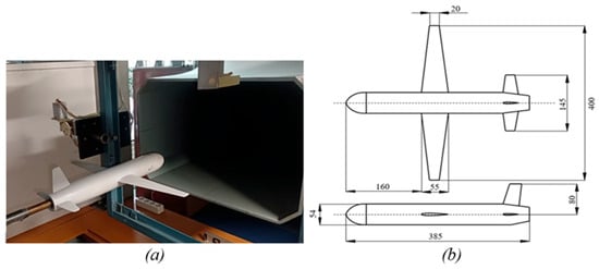
Figure 8. Experimental model in the wind tunnel: (a) Installation of the model in the wind tunnel; (b) Geometric parameters of the experimental model.

The experiment was carried out under ambient conditions of pressure p = 736 mmHg, temperature T = 23.4 °C, and free-stream velocity V_∞ = 25.5 m/s. The model employed has geometric dimensions shown in Figure 9b, and the airfoil used is NACA 1115.

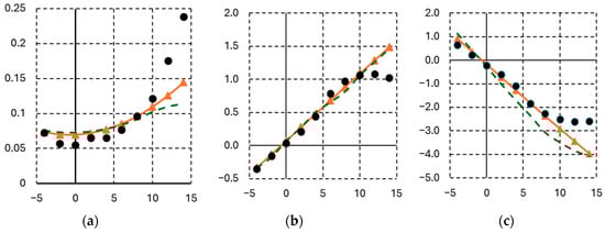
Figure 9. Aerodynamic characteristics: (a) Dependence of C_D on α; (b) Dependence of C_L on α; (c) Dependence of C_M on α.

The aerodynamic coefficients obtained using OpenVSP software and the constructed MLP network are compared with the experimental data in Figure 9.

Two commonly used statistical metrics were employed to assess the accuracy of the predicted aerodynamic coefficients: the mean absolute error and the Root Mean Square Error. Table 13 summarizes the corresponding results.

Table 13. Accuracy of aerodynamic characterization between MLP and experiment.

	RMSE	MAE	RMSE/MAE
CD	0.0123	0.0109	1.1274
CL	0.0799	0.0600	1.3306
CM	0.5879	0.5149	1.1418

Overall, the consistently low RMSE/MAE ratios (ranging from 1.1 to 1.3) indicate that the error distribution across all coefficients remains stable and well-controlled. Although a higher absolute error is observed for C_M, the results are scientifically reasonable and can be regarded as sufficiently accurate for preliminary aerodynamic analyses and optimization studies.

The experiment showed that at angles of attack of more than 10°, a nonlinear section of the dependence of lift on the angle of attack appears due to the separation of the flow on the wing. Numerical mathematical models used to calculate the database in the linear stationary formulation. Despite taking into account the effect of air viscosity on aerodynamic drag, the models do not take into account the effect of viscosity on the separated flow characteristics of the wing. This is expressed in a linear increase in lifting force at α > 10°, where the experiment shows a decrease in lifting force due to flow separation, and is also expressed in an underestimated resistance at α > 10° due to the inability to account for separation flow. The authors of fundamental works [29,30] note the applicability of these models in a linear formulation in the range of −10° < α < +10°. This circumstance limits the use of the developed surrogate models to a range of angles of attack of −10… + 10°, which, however, is quite sufficient for aerodynamic analysis and optimization at the initial stages of designing non-maneuverable aircraft. For these reasons, when comparing, experimental points at angles of attack of 12 and 14 degrees were not considered.

3.3. Solving an Applied Aerodynamic Design Problem Using MLP

We demonstrate the capability of the MLP-based aerodynamic model to address applied design problems in aeronautical engineering using the example of determining the longitudinal equilibrium of an aircraft in the vertical plane.

For an aircraft-type configuration with two lifting surfaces, the static longitudinal trim is achieved by adjusting the relative angular positions of the lifting surfaces in the longitudinal direction and the angle of attack of the overall lifting system at a given dynamic pressure. For convenience in considering different aerodynamic layouts, the incidence angle of the forward lifting surface is assumed constant, δ₁ = const. In this case, the relative angular position of the lifting surfaces is defined by the incidence angle of the rear lifting surface. Accordingly, the condition of static equilibrium of the aircraft in the vertical plane during steady horizontal flight can be expressed as follows:

$$\left\{\begin{array}{c}{C}_m\left(\alpha , {\delta }_2\right)=0 \\ C_L\left(\alpha , {\delta }_2\right)=C_{Lbal}\\ D=T \end{array}\right.,$$

(4)

where C_m is the pitching moment coefficient of the aircraft, C_L is the lift coefficient of the aircraft, C_Lbal is the lift coefficient required to balance the aircraft weight, α is the angle of attack of the lifting system, δ₂ is the incidence angle of the rear lifting surface, D is the aerodynamic drag of the aircraft, and T is the thrust produced by the propulsion system.

Figure 10 schematically illustrates the longitudinal trim of the aircraft in the vertical plane using the variables α and δ₂.

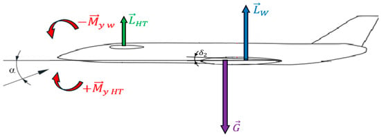
Figure 10. Scheme of longitudinal trim of an aircraft with an arbitrary aerodynamic configuration in the vertical plane.

The solution of problem (4) was carried out in terms of the NLP in the following formulation:

$$\begin{gathered} \left|{\mathrm{C}}_{\mathrm{M}}\left({\mathrm{x}}^{\mathrm{o}\mathrm{p}\mathrm{t}}\right)\right|\le \left|{\mathrm{C}}_{\mathrm{M}}\left(\mathrm{x}\right)\right| \forall \mathrm{x}\in \mathsf{\Omega }, \\ \mathsf{\Omega }=\left\{\mathit{x}: C_L\left(\mathit{x}\right)=C_{L,bal}\right\} \end{gathered}$$

(5)

where $C_M\left(\mathit{x}\right)$ is the objective function (pitching moment coefficient); $\mathit{x}=\left\{\alpha ,{\delta }_2\right\}$ is the vector of variables; ${\mathit{x}}^{\mathit{o}\mathit{p}\mathit{t}}$ is the optimal solution of the problem; and Ω is the feasible design space.

The solution search was performed using the COBYLA (Constrained Optimization By Linear Approximation) algorithm [37,38], implemented in the OpenMDAO library in Python [39].

The trim solution was analyzed for 100 aerodynamic configurations randomly generated using LHS, obtained from combinations of 23 parameters within the considered range (Table 1 and Table 2), in the optimization problem formulation (5). In this problem, C_Lbal = 0.5 and C_m = 0 were assumed.

The evaluation of the objective function and constraints in (5) was performed using the MLP-based aerodynamic model. To assess the reliability of the obtained results, Figure 11 and Figure 12 present a comparison with the corresponding solution of the same problem obtained using the same optimization algorithm, but with the objective function computed from numerical models in OpenVSP.

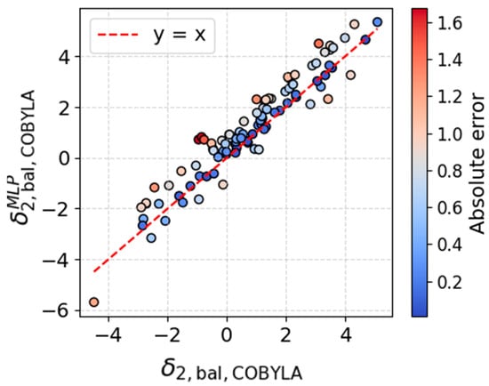
Figure 11. Comparison of installation angle.

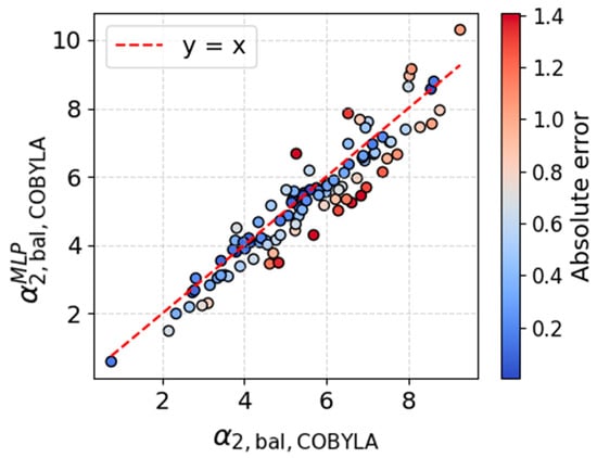
Figure 12. Comparison of angle of attack.

For both target variables, α and δ₂, the data points are scattered along the line of equality (y = x), indicating an overall strong correlation between the values predicted by the MLP and those computed from numerical models, as well as the absence of systematic bias. The deviation of the predicted values of α and δ₂ obtained with the MLP from those computed numerically does not exceed, on average, 1–1.5°, which demonstrates an acceptable level of predictive reliability, particularly considering the complexity of the modeled aerodynamic processes.

One of the key advantages of using the MLP, compared to numerical aerodynamic models in OpenVSP, is the significantly shorter computation time: the calculation of the equilibrium state for 100 aerodynamic configurations using the MLP required 2 min, whereas numerical simulations took 4 h. Both calculations were performed on a standard office computer (Intel(R) Core(TM) i7-6700 @ 3.40 GHz, 64 GB RAM) utilizing two cores.

The mean absolute errors of the remaining aerodynamic coefficients for the 100 considered configurations at the obtained values of α and δ₂ are presented in Table 14.

Table 14. Mean absolute errors of the remaining aerodynamic coefficients obtained using the direct MLP model and the numerical method.

$\Delta$CD	$\Delta {\mathit{C}}_{\mathit{l}}^{\mathit{\beta }}$	${\Delta \mathit{C}}_{\mathit{n}}^{\mathit{\beta }}$	$\Delta {\mathit{C}}_{\mathit{m}}^{{\mathit{C}}_{\mathit{L}}}$	${\Delta \mathit{C}}_{\mathit{m}}^{{\mathit{\omega }}_{\mathit{y}}}$
0.002572	0.028501	0.036966	0.015536	3.038369

4. Conclusions

The results demonstrated the advantages of using neural networks over numerical mathematical models for calculating the aerodynamic characteristics of aircraft, primarily due to the substantial acceleration of computations. The examples considered in this study show that MLP-based surrogate aerodynamic models significantly reduce computation time: a single direct calculation is performed approximately 600 times faster.

The proposed method of geometric discrete parameterization of aircraft aerodynamic configurations enabled the generation of a training dataset for the MLP with several samples based on combinations of 23 parameters. This enabled the development of a sufficiently accurate and generalized neural network model capable of handling conventional, canard, and tandem aircraft configurations with various combinations of discrete and continuous parameters.

The capabilities of neural network models for solving applied problems have been demonstrated. A significant acceleration (approximately 600-fold) of the aircraft longitudinal trim process has been demonstrated. The absolute computation time for trimming a single aircraft using surrogate models is about 1 s, compared to 2.5 min with numerical models employing the vortex lattice method. This computational speedup opens new opportunities for addressing a range of specific problems. These include optimization studies at the early stages of aircraft design, when many design alternatives must be evaluated within a short time frame, and flight dynamics and ballistics problems, where real-time solutions are required.

Furthermore, the performance of the surrogate model scales well for large-scale computations. For example, a 100-fold increase in the number of computations results in a computation time increase in less than 1%. Meanwhile, numerical mathematical models demonstrate a nearly directly proportional increase in computation time with the volume of computations, and the use of parallel processes limits the increase in computation speed through the number of processor cores.

The accuracy of neural network models depends not only on the quality of training and careful optimization of the hyperparameters of the neural network architecture, but also on the quality of the data in the database, which in turn strongly depends on the ability of numerical mathematical models to simulate physical processes in aerodynamics in detail. This is clearly seen from the results of validation of the neural network model based on experimental data: the neural network predicts aerodynamic characteristics well only in the operating range of the mathematical model used (Table 13, Figure 9). Nevertheless, the mathematical models used made it possible to obtain a database for training a neural network in a fairly short time in order to show new possibilities in accelerating aerodynamic calculations. The achieved accuracy of the neural network model is sufficient for the initial stages of aircraft engineering design. Further refinement of the neural network model is possible by preparing a database based on more detailed mathematical models of aerodynamics, for example, using solutions to the Navier-Stokes equations.

Further research in this field should focus on predicting not only integral but also distributed aerodynamic characteristics. This would make it possible to reduce the computation time of loads required for structural strength and weight analyses of the aircraft at the early stages of design.

References

- Komarov, V.A.; Weisshaar, T.A. New Approach to Improving the Aircraft Structural Design process. J. Aircr. 2002, 39, 227–233. [Google Scholar] [CrossRef]
- Eger, S.M.; Liseytsev, N.K.; Samoilovich, O.S. Osnovyi Avtomatizirovannovo Proektirovaniya Samoletov [Fundamentals of Automated Design of Aircraft]; Mashinostroenie Publishers: Moscow, Russia, 1986; 232p. [Google Scholar]
- Lazarev, I.B. Osnovyi Optimal’novo Proektirovaniya Konstruksiy. Zadachi i Metodyi [Fundamentals of Optimal Design of Structures. Problems and Methods]; Siberian State Academy of Railway Engineering: Novosibirsk, Russia, 1995; 295p. [Google Scholar]
- Łukaszewicz, G.; Kalita, P. Navier–Stokes Equations: An Introduction with Applications; Springer International Publishing: Cham, Switzerland, 2016; 390p. [Google Scholar]
- Chen, S.; Doolen, G.D. Lattice Boltzmann Method for Fluid Flows. Annu. Rev. Fluid Mech. 1998, 30, 329–364. [Google Scholar] [CrossRef]
- Dong, Y.; Tao, J.; Zhang, Y.; Lin, W.; Ai, J. Deep Learning in Aircraft Design, Dynamics, and Control: Review and Prospects. IEEE Trans. Aerosp. Electron. Syst. 2021, 57, 2346–2368. [Google Scholar] [CrossRef]
- Sekar, V.; Khoo, B.C. Fast flow field prediction over airfoils using deep learning approach. Phys. Fluids 2019, 31, 057103. [Google Scholar] [CrossRef]
- Moin, H.; Khan, H.Z.I.; Mobeen, S.; Riaz, J. Airfoil’s Aerodynamic Coefficients Prediction using Artificial Neural Network. In Proceedings of the 19th International Bhurban Conference on Applied Sciences and Technology (IBCAST), Islamabad, Pakistan, 16–20 August 2022; pp. 175–182. [Google Scholar]
- Kensley, B.; Ruben, S.; Oubay, H.; Kenneth, M. An Application of Neural Networks to the Prediction of Aerodynamic Coefficients of Aerofoils and Wings. Appl. Math. Model. 2021, 96, 456–479. [Google Scholar] [CrossRef]
- Huang, S.; Miller, L.; Steck, J. An Exploratory Airfoil Generation of Neural Networks to Airfoil Design; American Institute of Aeronautics and Astronautics (AIAA): Reston, VA, USA, 1994. [Google Scholar]
- Khurana, M.S.; Winarto, H.; Sinha, A.K. Application of Swarm Approach and Artificial Neural Networks for Airfoil Shape Optimization the Direct Numerical Optimization. In Proceedings of the 12th AIAA/ISSMO Multidisciplinary Analysis and Optimization Conference, Victoria, BC, Canada, 10–12 September 2008. [Google Scholar]
- Kharal, A.; Saleem, A. Neural Networks Based Airfoil Generation for a given Cp Using Bezier-PARSEC Parameterization. Aerosp. Sci. Technol. 2012, 23, 330–344. [Google Scholar] [CrossRef]
- Wang, J.; Li, R.; He, C.; Chen, H.; Cheng, R.; Zhai, C.; Zhang, M. An inverse design method for supercritical airfoil based on conditional generative models. Chin. J. Aeronaut. 2022, 35, 62–74. [Google Scholar] [CrossRef]
- Bouhlel, M.A.; He, S.; Martins, J.R.R.A. Based gradient–enhanced artificial neural networks for airfoil shape design in the subsonic and transonic regimes. Struct. Multidiscip. Optim. 2020, 61, 1363–1376. [Google Scholar] [CrossRef]
- Minaev, E.; Quijada Pioquinto, J.G.; Shakhov, V.; Kurkin, E.; Lukyanov, O. Airfoil Optimization Using Deep Learning Models and Evolutionary Algorithms for the Case Large-Endurance UAVs Design. Drones 2024, 8, 570. [Google Scholar] [CrossRef]
- Catalani, G.; Agarwal, S.; Bertrand, X.; Tost, F.; Bauerheim, M.; Morlier, J. Neural fields for rapid aircraft aerodynamics simulations. Sci. Rep. 2024, 14, 25496. [Google Scholar] [CrossRef]
- Chen, W.W.; Ramamurthy, A. Deep Generative Model for Efficient 3D Airfoil Parameterization and Generation. In Proceedings of the AIAA Scitech 2021 Forum, Virtual Event, 11–21 January 2021; p. 1690. [Google Scholar] [CrossRef]
- Espinosa Barcenas, O.U.; Quijada Pioquinto, J.G.; Kurkina, E.; Lukyanov, O. Surrogate Aerodynamic Wing Modeling Based on a Multilayer Perceptron. Aerospace 2023, 10, 149. [Google Scholar] [CrossRef]
- Lukyanov, O.; Hoang, V.H.; Kurkin, E.; Quijada-Pioquinto, J.G. Atmospheric Aircraft Conceptual Design Based on Multidisciplinary Optimization with Differential Evolution Algorithm and Neural Networks. Drones 2024, 8, 388. [Google Scholar] [CrossRef]
- Prediction of Aerodynamic Coefficients for Wind Tunnel Data Using a Genetic Algorithm Optimized Neural Network [Electronic Resource]. Available online: https://ntrs.nasa.gov/api/citations/20030107271/downloads/20030107271.pdf (accessed on 2 November 2024).
- Zan, B.; Han, Z.; Xu, C.; Liu, M.; Wang, W. High-dimensional aerodynamic data modeling using a machine learning method based on a convolutional neural network. Adv. Aerodyn. 2022, 4, 39. [Google Scholar] [CrossRef]
- Cavus, N. Aircraft Design Optimization with Artificial Intelligence. In Proceedings of the 54th AIAA Aerospace Sciences Meeting, San Diego, CA, USA, 4–8 January 2016. [Google Scholar] [CrossRef]
- Cavus, N. Artificial intelligence in aircraft conceptual design optimisation. Int. J. Sustain. Aviat. 2016, 2, 119–127. [Google Scholar] [CrossRef]
- Atmaja, S.T.; Fajar, R.; Aribowo, A. Optimization of deep learning hyperparameters to predict amphibious aircraft aerodynamic coefficients using grid search cross validation. AIP Conf. Proc. 2023, 2941, 020008. [Google Scholar] [CrossRef]
- Trani, A.; Wing-Ho, F. Enhancements to SIMMOD: A Neural Network Model to Estimate Aircraft Fuel Consumption; Phase I Final Report; Department of Civil Engineering Virginia Tech: Blacksburg, VA, USA, 1997. [Google Scholar]
- Trani, A.; Wing-Ho, F.; Schilling, G.; Baik, H.; Ses, A. A Neural Network Model to Estimate Aircraft Fuel Consumption. In Proceedings of the AIAA 4th Aviation Technology, Integration and Operations (ATIO) Forum, Chicago, IL, USA, 20–22 September 2004. [Google Scholar] [CrossRef]
- Secco, N.R.; de Mattos, B.S. Artificial neural networks to predict aerodynamic coefficients of transport airplanes. Aircr. Eng. Aerosp. Technol. Int. J. 2017, 89, 211–230. [Google Scholar] [CrossRef]
- OpenVSP. Available online: https://openvsp.org/ (accessed on 13 October 2023).
- Belocerkovskij, S.M. Tonkaya Nesushchaya Poverhnost’ V Dozvukovom Potoke Gaza [Thin Bearing Surface in Subsonic Gas Flow]; Nauka: Moscow, Russia, 1965; p. 244. [Google Scholar]
- Katz, J.; Plotkin, A. Low-Speed Aerodynamics, 2nd ed.; Cambridge Aerospace Series; Cambridge University Press: Cambridge, UK, 2001. [Google Scholar]
- Viana, F.A.C. A tutorial on Latin hypercube design of experiments. Qual. Reliab. Eng. Int. 2016, 32, 1975–1985. [Google Scholar] [CrossRef]
- Sheikholeslami, R.; Razavi, S. Progressive Latin Hypercube Sampling: An efficient approach for robust sampling-based analysis of environmental models. Environ. Model. Softw. 2017, 93, 109–126. [Google Scholar] [CrossRef]
- Spearman, C. The proof and measurement of association between two things. Am. J. Psychol. 1904, 15, 72–101. [Google Scholar] [CrossRef]
- Daniel, W.W. Spearman Rank Correlation Coefficient. Applied Nonparametric Statistics, 2nd ed.; PWS-Kent: Boston, MA, USA, 1990; pp. 358–365. [Google Scholar]
- Karali, H.; Inalhan, G.; Demirezen, M.U.; Yukselen, M.A. A new nonlinear lifting line method for aerodynamic analysis and deep learning modeling of small unmanned aerial vehicles. Int. J. Micro Air Veh. 2021, 13, 1–24. [Google Scholar] [CrossRef]
- Lukyanov, O.E.; Tarasova, E.V.; Martynova, V.A. Remote Control of Experimental Installation and Automation of Experimental Data Processing; Samara Scientific Center of the Russian Academy of Sciences: Samara, Russia, 2017; pp. 128–132. [Google Scholar]
- Powell, M.J.D. A Direct Search Optimization Method That Models the Objective and Constraint Functions by Linear Interpolation. In Advances in Optimization and Numerical Analysis. Mathematics and Its Applications; Gomez, S., Hennart, J.P., Eds.; Springer: Dordrecht, The Netherlands, 1994; Volume 275. [Google Scholar] [CrossRef]
- Barcenas, O.U.E.; Pioquinto, J.G.Q.; Kurkina, E.; Lukyanov, O. Multidisciplinary Analysis and Optimization Method for Conceptually Designing of Electric Flying-Wing Unmanned Aerial Vehicles. Drones 2022, 6, 307. [Google Scholar] [CrossRef]
- Gray, J.S.; Hearn, T.A.; Moore, K.T.; Hwang, J.T.; Martins, J.R.R.A.; Ning, A. OpenMDAO: An open-source framework for multidisciplinary design, analysis, and optimization. Struct. Multidiscip. Optim. 2019, 59, 1075–1104. [Google Scholar] [CrossRef]
Disclaimer/Publisher’s Note: The statements, opinions and data contained in all publications are solely those of the individual author(s) and contributor(s) and not of MDPI and/or the editor(s). MDPI and/or the editor(s) disclaim responsibility for any injury to people or property resulting from any ideas, methods, instructions or products referred to in the content. |
© 2025 by the authors. Licensee MDPI, Basel, Switzerland. This article is an open access article distributed under the terms and conditions of the Creative Commons Attribution (CC BY) license (https://creativecommons.org/licenses/by/4.0/).