Abstract
Kidney disease is a social and global health concern where early detection is crucial to reducing mortality and improving treatment outcomes. Traditional diagnostic methods are time-consuming and prone to human error. To address the issue, this study proposes an efficient automated deep learning diagnostic system using medical imaging for kidney disease detection and classification. The framework integrates DenseNet121 and EfficientNetB0 for deep feature extraction, followed by SVM, Random Forest, and XGBoost classifiers combined via soft voting. The proposed system was evaluated on 12,446 CT images encompassing four kidney classes: cyst, stone, tumor, and normal. The proposed model achieved outstanding performance metrics with an accuracy of 99.24% and an F1-score of 99%. The proposed model enables early and accurate detection of kidney disease, aiding timely treatment, especially in resource-limited settings.
1. Introduction
Kidney disease has become a major health concern affecting millions of individuals worldwide. The number of people suffering from chronic kidney disease (CKD) and related disorders, such as tumors, stones, and cysts, has been growing rapidly in recent years [1]. CKD affects over 10% of the global population. The recent estimates showed that between 700 and 850 million people in the world have the condition [2,3]. Furthermore, some conditions, like multilocular kidney cysts and stones, may recur or remain undetectable in their earliest stages, adding additional diagnostic complexities. Renal cancers, or kidney tumors, constitute approximately 2.5% of all cancer cases [4]. Simple cysts are common (especially with increasing age), but the number may be higher in certain genetic or acquired disease states (e.g., CYP24A1 deficiency, dialysis-associated acquired cystic kidney disease), and possibly increase in CKD progression and cancer risk [5,6]. The incidence of kidney cancer is rising worldwide, with approximately 400,000 new cases annually and 175,000 deaths. The causes are CKD, acquired cystic kidney diseases, and metabolic disorders. Kidney malignancies comprising Wilms’ tumor appear as 3–11% in all childhood cancers [7,8]. Kidney stones account for one of the predominant causes of CKD, affecting approximately 10% of adults worldwide, with recurrence rates reaching up to 50% [9,10]. Early detection of CKD is vital because most times, the conditions of CKD go unnoticed, which makes people unaware in the early stages. Identifying CKD in the early stages allows for timely interventions that can slow or even halt disease progression, reduce the risk of complications such as cardiovascular disease, improve overall patient outcomes, and increase survival rates [11,12]. A deep neural network (DNN) model with a limited dataset may increase the probability of overfitting [13]. Traditional diagnostic methods, such as blood tests and biopsies, are often invasive, time-consuming, and may fail to accurately identify early-stage kidney diseases [14]. Traditional diagnostic methods and standalone machine learning models face challenges such as overfitting, slow computational speed, class imbalance, and limited feature extraction capabilities, which hinder their effectiveness in clinical settings [15,16]. Due to the time-consuming registration, the processing speed of the model becomes slow, hampering the model’s practicality for real-time clinical use, and loses its validation [17]. Deep learning methods, particularly CNNs, have proven their worth in various applications related to medical image classification [18]. CNNs would be able to analyze kidney images obtained from ultrasound, MRI, and CT for the identification of abnormalities with a high degree of accuracy [19]. Despite the great advance in CNN-based kidney disease classification, several intrinsic drawbacks are still inherited from past research. Most of the existing studies simply focus on employing a single CNN model, such as VGG, ResNet, or Inception, without presenting an extensive comparison or fusion of different feature extractors. In addition, very little effort has been given to explaining the selection of some CNN models and their parameter adjustment, which usually influences the explainability and transferability of the results. Class imbalance is rarely fully addressed, and experiments rarely evaluate model robustness under different data partition ratios or on different datasets. Second, the lack of full ablation studies and thorough analyses of existing methods makes the identification of the optimal feature fusion and classification methods hard to find. These call for a more formal, interpretable, and robust hybrid scheme that can integrate complementary CNN structures for improving the reliability of diagnoses in kidney disease detection. Hybrid deep learning approaches fix these limitations by synthesizing the strength of deep learning in robust feature extraction with the strengths of classical machine learning or optimization algorithms in efficient and accurate classification, leading to improved diagnostic accuracy, reduced computational load, and better handling of imbalanced datasets [15,20].
This study proposes a hybrid deep learning model for the accurate classification of kidney diseases from medical images. It also explores effective feature extraction techniques, investigates the benefits of transfer learning with pretrained CNN architectures, and prioritize improvements in both model performance and interpretability to enhance clinical usability. The model combines the extracted features of DenseNet121 and EfficientNetB0 effectively, and the Synthetic Minority Oversampling Technique (SMOTE) is applied to handle class imbalance in the dataset. In order to further refine the process of classification, three machine learning classifiers is applied, Support Vector Machine (SVM), Random Forest (RF), and eXtreme Gradient Boosting (XGBoost). A soft-voting ensemble mechanism is applied subsequently in order to leverage the performance of individual models as well as combined prediction accuracy and reliability. The hybrid model with an ensemble classifier correctly classifies kidney diseases with abnormalities and achieved an outstanding performance, suggesting the effectiveness and readiness of the model for real-world deployment in computer-aided kidney disease diagnosis. To further evaluate the model, it was tested on two more augmented datasets in which it performed well. Thus, this study provides a hybrid model with the following contributions:
- This study combines DenseNet121 and EfficientNetB0, both state-of-the-art convolutional neural networks, and they efficiently extract dense and discriminative features from medical images.
- By combining deep learning models and traditional machine learning algorithms, the hybrid model benefits from the representational power of CNNs and the interpretability and generalizability of conventional classifiers.
- A novel soft-voting ensemble strategy is introduced to fuse multiple classifier outputs, enhancing the model’s stability and diagnostic reliability across heterogeneous datasets.
- The proposed pipeline incorporates a class-balancing mechanism using the Synthetic Minority Oversampling Technique (SMOTE), ensuring equitable learning across imbalanced medical image categories and improving generalization for underrepresented kidney disease types.
The rest of the article is organized as follows: Section 2—Related work—reviews of the background, motivation, and research gaps. Section 3—Methodology—explains the workflow diagram. Section 4—Experimental setup—states the evaluation metrics and device configuration. Section 5—Results and discussion—explains results, comparing CNN models for kidney disease classification across imaging modalities. Finally, Section 6—Conclusion—summarizes the limitations and future research directions.
2. Related Work
Deep learning medical image analysis started with core architectures, including AlexNet [21], VGGNet [22], GoogLeNet [23], ResNet [24], and other similar models. The research demonstrated how convolutional neural networks (CNNs) could extract multi-level image features which led to new medical diagnostic approaches. Medical imaging performance for segmentation tasks received a major boost from U-Net [25], which became a standard architecture. The classical models formed the foundation for modern networks like DenseNet and EfficientNet, which deliver better feature sharing and depth utilization and gradient flow for superior disease detection accuracy. Deep learning methods have been broadly used for the automated detection and classification of kidney abnormalities in medical imaging. However, many earlier approaches, as given in Table 1, show limited generalizability across diverse imaging modalities and patient populations. A deep neural network was proposed by Cruz et al. combining AlexNet for scope reduction and U-Net for segmentation, achieving a high accuracy of 99.92% on the KiTS19 dataset; parameter settings are manually defined, which may lead to the loss of kidney slices or small true positives, thereby reducing segmentation accuracy [26]. A VGG-19-based hybrid model was proposed by Somasundaram et al. Comparing the hybrid model with AlexNet, GoogLeNet, ResNet, and SqueezeNet for kidney stone detection, it achieved a high accuracy of 99.89% and lacked evaluation across diverse datasets, which may affect the model’s generalizability to different medical imaging conditions [27].A U-Net-based deep learning model was developed by Choudhari et al. for the semantic segmentation of kidneys and tumors, demonstrating strong IOU scores, but tumor segmentation accuracy was low, which indicated that additional training epochs and model optimization were needed to improve performance [28].

Table 1.
Summary of models, advantages, and limitations in kidney disease detection.
Patro et al. suggested a Kroneker product-based convolution approach for reducing feature map redundancy and avoiding convolutional overlap, achieving an accuracy of 98.56%, but it is not cost-effective [29]. AI-powered healthcare systems in resource-poor settings are suggested by Ekpar et al., which face limitations such as infrastructure and low digital literacy [30]. Subedi et al. use Vision Transformer (ViT), which sets the boundaries for traditional methods and demonstrates the promise of potential improvement in the medical image analysis field but has not been tested yet on varied datasets [31]. Yildrim et al. proposed a deep learning model which could assist radiologists to detect kidney stone cases accurately and it was clinically proven, but the kidney stones could not be classified according to the sizes [32]. Ghosh et al. developed a fuzzy inference system to enhance kidney CT image contrast with an accuracy of 99.2%, but their dataset was limited and did not have tumor localization and was not clinically validated [33]. An inductive transfer-based ensemble deep neural network (DNN) was used by Chaki et al. for feature extraction, but it lacks spatial localization and has not been clinically tested yet [34].
A hybrid convolutional neural network (CNN) and Residual Network (ResNet) model introduced by Kumar et al. to combine the strengths of both networks achieved accuracy of 90% but lacked multi-modal data integrity and interpretability [35]. Fuladi et al. suggested a CNN model which is limited by dataset diversity and lacks clinical validation, achieving an accuracy of 99.57% [36]. Recently, hybrid deep learning methods have been recognized for their ability to combine the strengths of different architectures. Majid et al. integrated DenseNet121 and ResNet50 to enable both fine-grained feature extraction and robust classifier training, yielding a significant improvement in diagnostic accuracy, but their work was confined to a single dataset [37]. Furthermore, methods employing Grad-CAM and other interpretability techniques suggested by Asif et al. aid in understanding which image regions contribute most to the algorithm’s decisions, thereby strengthening clinician confidence in automated diagnostics but sometimes misclassifying CT images, which can pose severe clinical risks [38]. A CNN-based deep learning approach was proposed by Chanakya et al. for the automated detection of kidney diseases, improving the decipher capacity with an accuracy 98.66% [39]. Ensembles of three deep learning models and three vision transformers were proposed by Ayogu et al., achieving a high accuracy of 99.67%, but the absence of object detection techniques in the preprocessing stage may restrict the ability of the model [40].
Refaee et al. proposed a machine learning approach named ResNet-50, which enhanced early detection, achieving an accuracy of 83%, but the study lacked a diverse dataset; the implementation of XAI may increase the model’s performance [41]. Reddy et al. introduced a deep network comparing U-Net for segmentation and AlexNet for classification, reporting 94.75% accuracy with AlexNet, and they visualized the convolutional layers using saliency maps [42]. A deep learning approach named DarkNet53 was proposed by Obaid et al. for leveraging and generating best performance, but the model fully depended on high-quality and diverse datasets, which may hinder its accuracy in low-resource settings [43]. To enhance the early detection and classification of kidney diseases, a deep learning approach was proposed by Pimpalkar et al., achieving an accuracy of 99.96%, but the study lacked cross-dataset evaluation [44]. An ensemble of CNN models was proposed by Saber et al., achieving an accuracy of 99.85%, but the study lacked external dataset validation, which may restrict the model’s reliability [45].
The medical field has seen multiple deep learning systems achieve outstanding results. The effectiveness of CNNs, U-Net, and hybrid frameworks appears in multiple studies [26,28,37,42,44,45]. However, these studies base their findings on restricted dataset samples, which makes their models unsuitable for different medical environments. The models from Somasundaram et al. [27] and Fuladi et al. [36] achieve high accuracy results, but they have not been tested on external datasets or through cross-dataset evaluation. The architectures from Patro et al. [29] and Kumar et al. [35] deliver strong results, but their systems operate at high computational costs and produce results that lack interpretability. The implementation of Grad-CAM and saliency map techniques [38,42] improves system transparency, but these methods produce incorrect classifications of essential CT areas, which could lead to dangerous medical outcomes. The current models do not solve actual problems that stem from restricted infrastructure and insufficient digital skills in underdeveloped areas [30,43]. Despite significant progress, the literature reveals persistent gaps: (1) limited generalization across multiple datasets, (2) lack of interpretability and clinical validation, and (3) insufficient exploration of complementary hybrid feature extraction. To address these gaps, this study introduces a hybrid model combining DenseNet121 and EfficientNetB0, designed to enhance feature diversity, interpretability, and classification robustness, yielding a reliable and trustworthy pipeline for automated kidney disease detection and classification.
3. Methodology
This research work maintains a systematic workflow illustrated in Figure 1 that includes several steps: (a) data collection, (b) data preprocessing and enhancement, (c) feature extraction, (d) SMOTE balancing, (e) classification and prediction, and (f) visualization.
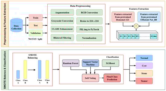
Figure 1.
Methodology flow diagram of proposed architecture.
Initially, the images were enhanced by using two techniques, Contrast-Limited Adaptive Histogram Equalization (CLAHE) and bilateral filtering, then used two distinct feature extractors—Densenet121 and EfficientNetB0. DenseNet121 was chosen for its dense connectivity, which facilitates efficient gradient flow and feature reuse, while EfficientNetB0 provides balanced depth, width, and resolution scaling for parameter efficiency. Their complementary structures enable the fusion of multi-scale and hierarchical features, enhancing robustness for kidney disease detection.
SMOTE balancing was used to reduce class imbalance. Although SMOTE is primarily designed for tabular data, its application to deep feature vectors helps balance the class distribution in the latent feature space. This ensures that minority classes, such as kidney stones, are adequately represented without introducing artificial pixel-level artifacts. These features were then combined and fed into three machine learning classifiers, Support Vector Machine (SVM), Random Forest (RF), and XGBoost, to accurately detect and classify diseased kidneys.
3.1. Data Collection
The dataset used in this research consists of CT kidney images sourced from Kaggle (https://www.kaggle.com/datasets/nazmul0087/ct-kidney-dataset-normal-cyst-tumor-and-stone (accessed on 15 June 2025)). The dataset is publicly available and distributed under an open academic license on Kaggle, allowing reuse for research and publication purposes. All patient information was anonymized, ensuring compliance with ethical data usage standards. It includes four distinct classes—cyst (3709 images), normal (5077 images), stone (1377 images), and tumor (2283 images)—making a total of 12,446 labeled images. The dataset was split into a 70/15/15 ratio for training, testing, and validation, as shown in Figure 2 below.
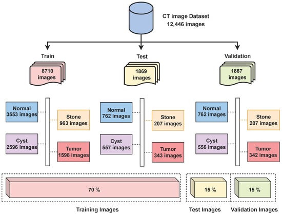
Figure 2.
Distribution of CT kidney images across classes.
While this partitioning provided satisfactory performance, the impact of alternative data split ratios such as 80/10/10 on model performance has not been fully explored. A comparative analysis using different partitioning strategies is planned for future work to assess the robustness and sensitivity of the proposed approach to data division.
All experiments in this study are conducted using variations of the same Kaggle CT kidney dataset. While the results demonstrate strong performance on this dataset, the generalizability of the proposed approach to other populations, imaging protocols, or clinical settings remains to be validated. Future work will involve testing the model on independent datasets from multiple sources to further assess its robustness and real-world applicability.
Some of the examples of the ct images of four classes are shown in Figure 3.
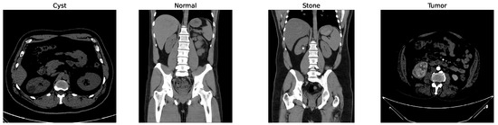
Figure 3.
Examples of cyst, normal, stone, and tumor CT image.
While other kidney diseases exist, this study specifically focuses on these four classes due to the availability and balance of labeled data in the dataset. Extension to additional diseases is left for future work.
3.2. Data Preprocessing
To improve contrast, reduce noise, and enable robust training, a series of preprocessing and augmentation steps was applied to the CT images. Each grayscale CT image was first enhanced using CLAHE to highlight fine-grained textures. CLAHE parameters were empirically selected with a clip limit of 2.0 and a tile grid size of (8, 8), which provided optimal contrast enhancement without amplifying noise. For bilateral filtering, parameters were set to diameter , , and , balancing smoothness with edge preservation. CLAHE operates by partitioning the image into small, non-overlapping regions and clipping their histograms at a predefined threshold T to avoid noise amplification. The clipped histogram is defined by , where denotes the original histogram count for bin i. The total excess C is evenly redistributed to all L histogram bins shown in Equation (1):
with and . Subsequently, the pixel intensities are remapped by their Cumulative Distribution Function (CDF) as per Equation (2):
Here, N represents the total number of pixels in the tile. This procedure efficiently improves the local contrast while avoiding noise and artifact enhancement. Bilateral filtering is then applied to reduce noise while preserving edges. This filter performs non-linear, edge-preserving smoothening by averaging nearby pixel intensities given in Equation (3):
with and representing the spatial and range kernel functions, denoting the neighborhood, and acting as a normalization factor. Figure 4 shows the changes in the image after applying the CLAHE and bilateral filtering.
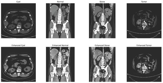
Figure 4.
CLAHE + bilateral filter enhanced image.
To further augment the dataset and aid in generalization, transformation techniques such as rotation, flipping, and zooming were applied [46]. All enhanced images were then resized to pixels, converted to RGB format, and normalized using ImageNet’s mean and standard deviation , expressed as Equation (4):
with I representing the pixel values. Normalization using ImageNet statistics ensures feature compatibility with pretrained CNNs, stabilizing learning and improving convergence. Augmentation techniques, including rotation, flipping, and zooming, further mitigate overfitting by providing geometric diversity. The processed and augmentated dataset was then fed in mini-batches to DenseNet121 and EfficientNetB0 for deep feature extraction. The resulting feature representations were concatenated and afterward classified using an ensemble of machine learning classifiers (Random Forest, SVM, and XGBoost) using soft voting.
Two more virtual datasets were created using separate augmentation technique to further validate the proposed model’s performance over varied data. The process of creating the virtual dataset is shown in Figure 5 below.
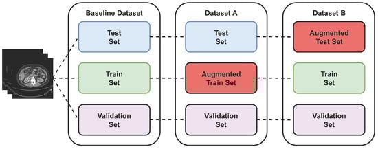
Figure 5.
Virtual dataset using augmentation technique.
3.3. Feature Extraction
Feature extraction is an important technique as it provides the most informative patterns for accurate diagnosis [47]. While several studies have applied single CNN architectures such as ResNet or VGG for kidney CT analysis, their limited feature diversity restricts generalization. The proposed hybrid feature extraction leverages both dense connections (DenseNet121) and compound scaling (EfficientNetB0) to capture complementary spatial and semantic representations, thus improving discriminative capacity. DenseNet121 introduces dense feature reuse and reduces the problem of vanishing gradients, while EfficientNetB0 relies on compound scaling for an ideal balance between accuracy and efficiency. Therefore, their complementary feature hierarchies allow for better texture sensitivity and lesion discrimination than VGG or ResNet, confirmed by preliminary experiments. In this study, a hybrid deep feature extraction approach was used, employing two well-established convolutional neural networks (CNNs)—DenseNet121 and EfficientNetB0—both pretrained in ImageNet. The classifier heads were removed, retaining their respective deep feature representations, which were subsequently fused into a unified descriptor for each CT image.
3.3.1. DenseNet121
DenseNet utilizes dense connections, expressed as Equation (5), where each layer directly accesses all previous feature maps:
with denoting concatenation of previous layer outputs and representing a composite operation. This architecture efficiently reuses features, reduces redundancy, and helps mitigate the vanishing gradient problem.
For feature extraction, we removed the classifier layer and used the output of the last pooling layer, which yielded a 1024-dimensional vector.
3.3.2. EfficientNetB0
EfficientNet utilizes a compound scaling method alongside depthwise separable convolutions (MBConv) and squeeze-and-excitation modules to enable lightweight yet powerful feature extraction. The last convolutional layer produces a 1280-dimensional vector.
3.3.3. Feature Fusion
To leverage the complementary representations of both networks, their respective feature vectors (1024- and 1280-dimensional) were concatenated as shown in Equation (6):
forming a unified 2304-dimensional descriptor. Feature concatenation was preferred over additive or attention-based fusion to preserve all discriminative information from both networks. Preliminary experiments showed that concatenation provided higher validation accuracy compared to other fusion methods. This fused vector was subsequently fed into classifiers (SVM, Random Forest, XGBoost) for robust and accurate kidney disease detection shown in Figure 6.
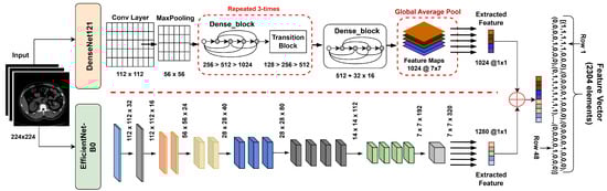
Figure 6.
Hybrid feature extractor concatenation with feature vector.
These classifiers are employed in a cascading ensemble manner, where each classifier contributes its predictions, which are then combined to form a stronger final decision. This approach leverages the complementary strengths of individual models, enhancing the overall classification performance.
3.4. SMOTE Balancing
To reduce the class imbalance problem of the stone class, which leads to more misclassifications, SMOTE is applied. A basic working principle of the SMOTE is illustrated in the Figure 7.
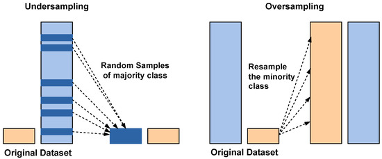
Figure 7.
Class balancing using undersampling and SMOTE oversampling. Blue bars: majority class; orange bars: minority class.
Traditionally, SMOTE is applied to input-level or shallow feature data to synthetically balance the classes. Applying it directly to high-dimensional deep feature embeddings can risk generating unrealistic samples. However, in this study, SMOTE was applied to the fused deep feature representations obtained by concatenating the outputs of DenseNet121 and EfficientNetB0. This design choice was motivated by the observation that the fused embeddings retained meaningful class separability in the high-dimensional feature space, allowing SMOTE to interpolate effectively between minority class neighbors.
Instead of simply duplicating minority class samples, SMOTE generates new synthetic examples by interpolating between existing minority class instances and their nearest neighbors. This process helps balance the dataset by increasing the representation of the minority class, thereby improving the model’s ability to learn meaningful patterns from underrepresented data. By reducing bias toward the majority class, SMOTE enhances the overall classification performance and ensures more reliable predictions in imbalanced learning tasks. To minimize the risk of unrealistic feature distributions after SMOTE augmentation, the generated feature vectors were inspected using dimensionality reduction visualization techniques like t-SNE on representative subsets, which indicated that synthetic features followed similar patterns to the original data.
3.5. Classification Models
After obtaining the 2304-dimensional fused feature vector from DenseNet121 and EfficientNetB0, traditional machine learning classifiers were used for final prediction, including Support Vector Machine (SVM), Random Forest (RF), and XGBoost. In practice, all classifiers were trained on the fused feature vectors with mostly default hyperparameters. Specifically, the SVM used an RBF kernel; Random Forest employed 100 estimators; and XGBoost used 200 boosting rounds with a default learning rate and maximum depth. Since these classifiers operate on fixed feature vectors, no batch size or training epochs were required. Finally, a soft-voting ensemble strategy was applied to combine their predictions and achieve greater robustness and accuracy.
3.5.1. Support Vector Machine (SVM)
SVM is a supervised algorithm which finds the hyperplane that maximally separates classes in high-dimensional space. In this study, radial basis function (RBF) kernel was used with a probability estimator and a fixed random state to ensure reproducibility.
3.5.2. Random Forest
Random Forest is an ensemble method that constructs multiple decision trees on different subsets of training data and merges their predictions, thereby reducing overfitting and improving generalization. Here, we used 100 trees with a set random state.
3.5.3. XGBoost
XGBoost is a high-performance algorithm based on gradient boosting and was also implemented with label encoding disabled and multiclass logarithmic loss as the evaluation metric, allowing for strong and accurate predictions.
To combine the strengths of these classifiers, a soft-voting ensemble was used, averaging their predicted class probabilities. The final class label was then assigned by choosing the highest average probability class. This approach resulted in a more balanced and robust classifier for kidney CT image recognition.
4. Experimental Setup
This section outlines the experimental setup adopted for model training and evaluation. It includes the metrics used for performance measurement and the technical configuration and tools used during implementation.
4.1. Evaluation Metrics
To comprehensively evaluate the performance of the proposed hybrid model, standard classification evaluation metrics were used, including Accuracy (), Precision, Recall, and F1-score.
Accuracy is the fundamental metric that shows the effectiveness of a model in making predictions [48]. It is represented by Equation (7):
Here, true positive () and true negative () represent the number of correctly classified positive and negative images, respectively. And false positive () and False Negative (), represents the number of positive and negative images that were incorrectly classified.
Precision is used to calculate the proportion of accurately predicted positive images related to the total predicted images within a positive class [49]. Precision is expressed as Equation (8):
Recall is the ratio of correctly predicted positive observations to all the actual positives. Recall is defined in Equation (9):
The F1-score, calculable by Equation (10) is an advanced accuracy metric that represents the weighted average of Precision and Recall, as it accounts for both false positives and false negatives [50].
4.2. Implementation Details
The experiments were conducted in Python (3.12.2) using TensorFlow (2.19.0)/Keras (3.7.0). Pretrained CNNs (e.g., DenseNet121 and EfficientNetB0) extracted features, and classifiers (SVM, RF, XGBoost) were trained with 42 random states and 100 estimators on a device equipped with Intel Core i7 11thGen 12gb RAM and 512gb SSD. The source code and preprocessed dataset splits will be made publicly available upon publication to ensure reproducibility and transparency.
5. Result and Discussion
During the training phase, 70% of 12,446 CT images were used for training and 15% for validation, which keeps track of whether the model is overfitting. After training, the remaining 15% is used for testing the model’s performance using 1869 images that were not used during the model train-up on the baseline dataset. This split provides a balanced evaluation between learning and unseen generalization. To further assess the robustness of the proposed model, two additional augmented datasets were created: Dataset A and Dataset B. This allowed an investigation of how training diversity and unseen augmentation influence model performance. The output of these three datasets is discussed in the following subsections.
As shown in Figure 8, the confusion matrix of the proposed hybrid model on the baseline dataset is presented below.
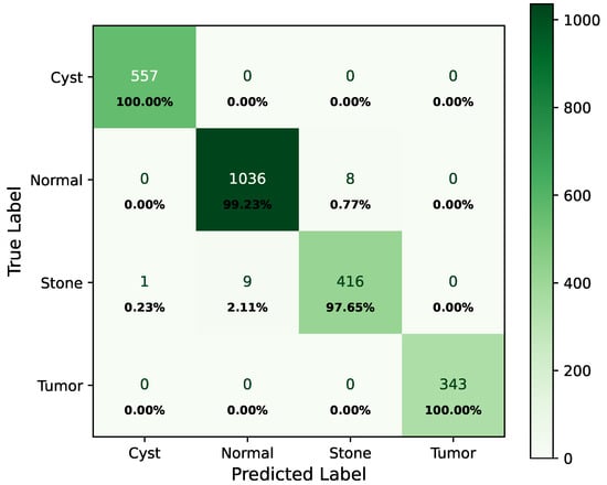
Figure 8.
Confusion matrix of baseline dataset.
In the matrix, the diagonal elements represent correctly classified instances, and the rest of the elements indicate misclassifications. The incorrectly classified numbers are 18, 18, and 21 for baseline, Dataset A, and Dataset B, respectively. Although the model performs consistently well across all datasets, a slightly higher misclassification rate is observed in the stone class. This is mainly attributed to the smaller sample size of the stone category, which limits the model’s ability to learn its feature variability, even after applying SMOTE balancing. Additionally, the visual inspection of misclassified cases shown in Figure 9 revealed that some stone images share overlapping visual characteristics with cyst and tumor classes, such as low-contrast textures and irregular boundaries, making them challenging to distinguish even for deep learning models.
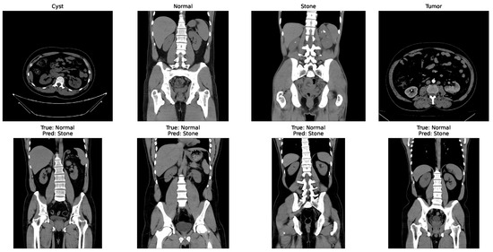
Figure 9.
Some incorrectly classified images.
The classification report of the baseline dataset is shown in Table 2.
Table 2.
Classification report on baseline dataset.
The AUC curve of the baseline dataset is shown in Figure 10.
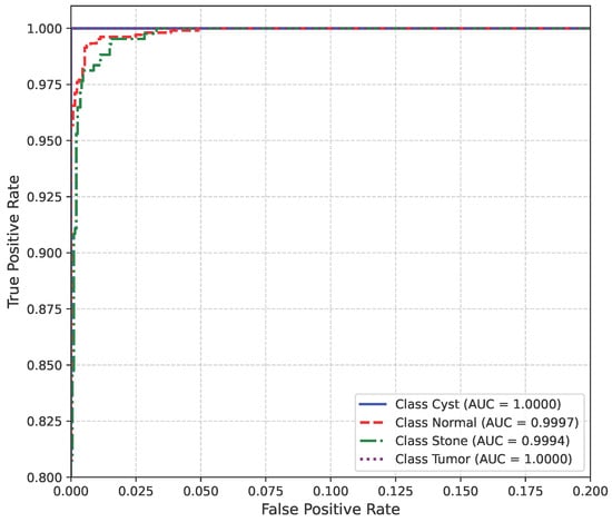
Figure 10.
AUC curve of baseline dataset.
The loss curve of the baseline dataset is shown in Figure 11.
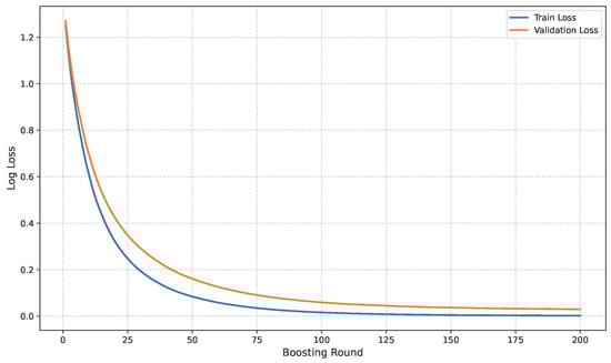
Figure 11.
Loss curve of baseline dataset.
Figure 12 shows the confusion matrix of Dataset A.
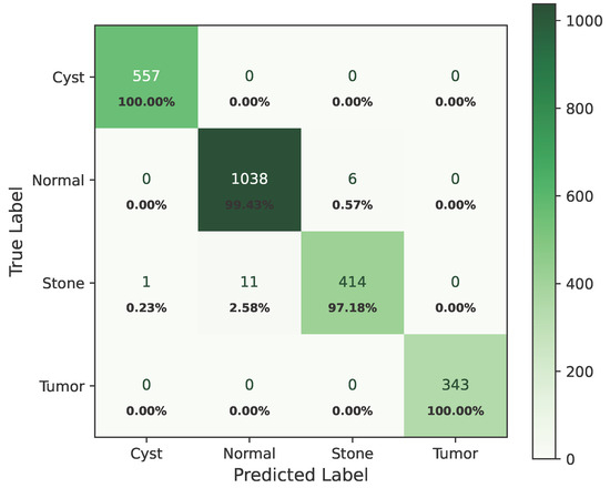
Figure 12.
Confusion matrix of Dataset A.
The classification report for Dataset A is presented in Table 3.
Table 3.
Classification report on Dataset A.
The AUC curve for Dataset A is shown in Figure 13.
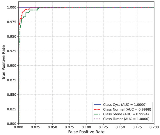
Figure 13.
AUC curve of Dataset A.
Figure 14 shows the loss curve for Dataset A.
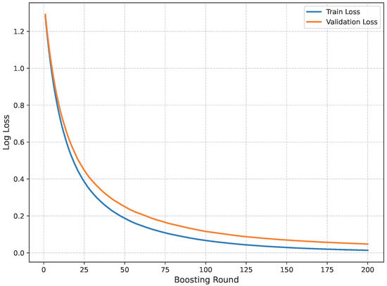
Figure 14.
Loss curve of Dataset A.
The confusion matrix of Dataset B is shown in Figure 15.
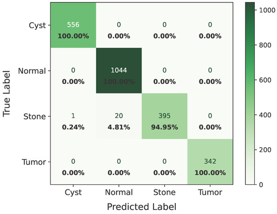
Figure 15.
Confusion matrix of Dataset B.
Table 4 presents the classification report of Dataset B.
Table 4.
Classification report on Dataset B.
Figure 16 shows the loss curve of Dataset B.
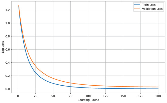
Figure 16.
Loss curve of Dataset B.
Figure 17 shows the AUC curve of Dataset B.
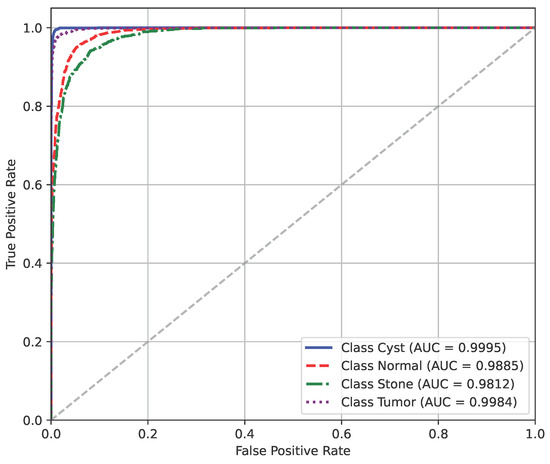
Figure 17.
AUC curve of Dataset B.
The model’s performance across the three datasets shows outstanding results on the baseline dataset, with an overall accuracy of 99.21% and near-perfect class-level performance, where all classes (cyst, normal, stone, tumor) obtained F1-scores between 0.98 and 1.00. On the contrary, almost similar results were observed on Dataset A, also achieving 99% accuracy, with only a slight decline in the stone class (F1 = 0.98), while the remaining classes, particularly cyst and tumor, maintained perfect scores. Dataset B contains augmented test samples with higher texture variability. As seen in the figures, the AUC values for all classes remain close to 1.0, indicating excellent discriminative ability. A high AUC demonstrates that the model can effectively differentiate positive and negative cases across all thresholds, providing a robust measure of performance beyond simple accuracy. The loss curves show smooth convergence without divergence between training and validation losses, suggesting that the model learned effectively without overfitting. This consistency across datasets confirms the regularizing effect of CLAHE, bilateral filtering, and SMOTE on improving generalization. Overall, while the model demonstrates impressive robustness on the baseline dataset and maintains it on Dataset A, the results on Dataset B identify the challenge in coping with more complex data distributions.
Table 5 presents a compact view of all the models that have been tested, including feature fusion strategies, a combination of classifiers, and performance metrics. Several architectures and classifier combinations were evaluated to justify the final model choice. DenseNet121 and EfficientNetB0 were selected due to their complementary characteristics—DenseNet’s dense connectivity promotes feature reuse and gradient stability, while EfficientNet’s compound scaling offers efficiency and fine-grained texture sensitivity.
Table 5.
Implemented approaches.
We implemented six single and four hybrid models combining different feature extractors and classifiers for kidney disease classification. Models like VGG-16 with Random Forest and ResNet-101 with Softmax performed moderately, while deeper architectures such as VGG-19 and ResNet-50 achieved higher accuracy by capturing finer features. DenseNet-121 and ResNet-101 performed best among single and dual models, reaching about 98% accuracy due to DenseNet’s dense connectivity and ResNet’s gradient stability.
An ablation study was conducted to assess the contribution of preprocessing, feature fusion, and classifier combination. CLAHE and bilateral filtering improved image clarity and contrast, enhancing feature extraction. The fusion of DenseNet121 and EfficientNetB0 further improved performance by combining dense and efficient feature representations. Finally, the tri-ensemble of Random Forest, SVM, and XGBoost outperformed individual classifiers, yielding the most stable and accurate predictions.
The final model—combining CLAHE, bilateral filtering, DenseNet-121, EfficientNet-B0, and the tri-ensemble classifier—achieved 99.24% accuracy, confirming the effectiveness of deep feature fusion and ensemble learning.
Finally the model is compared with existing studies in the same dataset, as shown in Table 6.
Table 6.
Evaluation of proposed model compared to existing methods.
From the comparison table, we can see that our proposed hybrid model achieves excellent results among all. There were two hybrid models, and among them, [37] achieved the best accuracy of 98.22%. There was a model named YOLO-v8 [51], whose accuracy was the lowest. On the contrary, our model—with CLAHE and bilateral filtering for top-of-the-line image enhancement, augmented by feature extraction from DenseNet121 and EfficientNet-B0 and backed by a robust ensemble classifier (Random Forest, SVM, and XGBoost)—reported a record level of 99.24% accuracy with a perfect 0.99 in Precision, Recall, and F1-score. This testifies to the unprecedented efficacy of the proposed hybrid and ensemble-based approach in presenting not just high accuracy but also uniform and stable performance in all classes, a new standard for kidney disease classification.
Finally, the comparative assessment firmly indicates the superiority of the suggested model over the current techniques in kidney disease classification. By utilizing the advanced preprocessing techniques (CLAHE and bilateral filtering), strong deep feature extractors (DenseNet121 and EfficientNet-B0), SMOTE class balancing, and a robust ensemble of classifiers (Random Forest, SVM, and XGBoost), the proposed model achieved an excellent accuracy of 99.24%, with near perfect Precision, Recall, and F1-score. This not only surpasses all the models reported earlier but also verifies the power of combining image enhancement, deep learning, and ensemble techniques in achieving strong and highly accurate medical image classification results.
6. Conclusions
In this study, a hybrid ensembled deep learning model was proposed for the detection and classification of kidney diseases using CT images. The model achieved 99.24% accuracy on 1869 images, with only 18 misclassifications. Also, on the other two augmented datasets, the model was 99.24% and 98.85% accurate with misclassifications of 18 and 21 cases, demonstrating that hybrid feature extraction with ensemble classification enables precise and automated kidney disease detection. Although the dataset is relatively balanced and class weight averaged using SMOTE, it is still a single-sourced dataset. Incorporating images from diverse scanners, acquisition settings, and rare disease types could enhance generalization. Cases where stone and tumor appearances are very similar may also benefit from domain-specific augmentation or clinical knowledge integration. The proposed method is suitable for resource-limited environments due to its lightweight preprocessing and use of pretrained feature extractors.
Future work will explore the integration of clinical metadata and real-time deployment to increase its utility across a wider range of clinical settings. Additionally, expanding the dataset and performing a more detailed error analysis could further strengthen the model’s generalizability and accuracy. Incorporating explainability modules such as Grad-CAM to enhance clinical interpretability will further strengthen confidence in automated diagnostic decision-making for real-world kidney disease detection.
Author Contributions
Conceptualization: M.B.A.M., M.N.H. and E.B.; data curation, formal analysis, investigation, methodology: M.N.H., E.B. and T.A.S.; funding acquisition, project administration: Z.M., M.F.A.M. and M.B.A.M.; resources, software: M.N.H., E.B. and T.A.S.; validation, visualization: M.B.A.M., M.N.H., E.B. and M.F.A.M.; writing—original draft: M.N.H., E.B., T.A.S. and M.B.A.M.; writing—review and editing: M.B.A.M., T.A.S., Z.M. and M.F.A.M. All authors have read and agreed to the published version of the manuscript.
Funding
This research received no external funding.
Institutional Review Board Statement
Not applicable.
Informed Consent Statement
Not applicable. The study used a publicly available de-identified dataset from Kaggle, collected with patient consent and confidentiality.
Data Availability Statement
The datasets used and/or analyzed during the current study are available from the corresponding author on reasonable request.
Conflicts of Interest
The authors declare no conflict of interest.
Abbreviations
The following abbreviations are used in this manuscript:
| CT | Computed Tomography |
| SVM | Support Vector Machine |
| RF | Random Forest |
| XGBoost | eXtreme Gradient Boosting |
| CKD | Chronic Kidney Disease |
| DNN | Deep Neural Network |
| CNN | Convolutional Neural Network |
| SMOTE | Synthetic Minority Oversampling Technique |
| AI | Artificial Intelligence |
| ViT | Vision Transformer |
| DL | Deep Learning |
| ML | Machine Learning |
| Grad-CAM | Gradient-weighted Class Activation Mapping |
| XAI | Explainable Artificial Intelligence |
| CLAHE | Contrast-Limited Adaptive Histogram Equalization |
| RBF | Radial Basis Function |
| ROC | Receiver Operating Characteristic |
| AUC | Area Under the Curve |
References
- Jha, V.; García-García, G.; Iseki, K.; Li, Z.; Naicker, S.; Plattner, B.W.; Saran, R.; Wang, A.; Yang, C.W. Chronic kidney disease: Global dimension and perspectives. Lancet 2013, 382, 260–272. [Google Scholar] [CrossRef]
- Kovesdy, C. Epidemiology of chronic kidney disease: An update 2022. Kidney Int. Suppl. 2022, 12 1, 7–11. [Google Scholar] [CrossRef]
- Deng, L.; Guo, S.; Liu, Y.; Zhou, Y.; Liu, Y.; Zheng, X.; Yu, X.; Shuai, P. Global, regional, and national burden of chronic kidney disease and its underlying etiologies from 1990 to 2021: A systematic analysis for the Global Burden of Disease Study 2021. BMC Public Health 2025, 25, 636. [Google Scholar] [CrossRef]
- Badawy, M.; Almars, A.; Balaha, H.; Shehata, M.; Qaraad, M.; Elhosseini, M. A two-stage renal disease classification based on transfer learning with hyperparameters optimization. Front. Med. 2023, 10, 1106717. [Google Scholar] [CrossRef]
- Hanna, C.; Potretzke, T.A.; Cogal, A.G.; Mkhaimer, Y.G.; Tebben, P.J.; Torres, V.E.; Lieske, J.C.; Harris, P.C.; Sas, D.J.; Milliner, D.S.; et al. High Prevalence of Kidney Cysts in Patients With CYP24A1 Deficiency. Kidney Int. Rep. 2021, 6, 1895–1903. [Google Scholar] [CrossRef] [PubMed]
- Shah, A.; Lal, P.; Toorens, E.; Palmer, M.; Schwartz, L.; Vergara, N.; Guzzo, T.; Nayak, A. Acquired Cystic Kidney Disease–associated Renal Cell Carcinoma (ACKD-RCC) Harbor Recurrent Mutations in KMT2C and TSC2 Genes. Am. J. Surg. Pathol. 2020, 44, 1479–1486. [Google Scholar] [CrossRef]
- Takahashi, J.; Tanaka, Y.; Sato, Y.; Ushiku, T.; Nishikawa, H.; Kume, H.; Mano, H. Abstract 6629: Spatial immunogenomic analysis of the transformation process in acquired cystic disease of the kidney. Cancer Res. 2025, 85, 6629. [Google Scholar] [CrossRef]
- Cirillo, L.; Innocenti, S.; Becherucci, F. Global epidemiology of kidney cancer. Nephrol. Dial. Transplant. 2024, 39, 920–928. [Google Scholar] [CrossRef]
- Singh, P.; Harris, P.; Sas, D.J.; Lieske, J. The genetics of kidney stone disease and nephrocalcinosis. Nat. Rev. Nephrol. 2021, 18, 224–240. [Google Scholar] [CrossRef] [PubMed]
- Siener, R. Nutrition and Kidney Stone Disease. Nutrients 2021, 13, 1917. [Google Scholar] [CrossRef] [PubMed]
- Vassalotti, J.; Francis, A.; dos Santos, A.C.S.; Correa-Rotter, R.; Abdellatif, D.; Hsiao, L.L.; Roumeliotis, S.; Haris, A.; Kumaraswami, L.A.; Lui, S.F.; et al. Are your kidneys ok? Detect early to protect kidney health. Ren. Fail. 2025, 47, 2503514. [Google Scholar] [CrossRef]
- Mizdrak, M.; Kumrić, M.; Kurir, T.; Božić, J. Emerging Biomarkers for Early Detection of Chronic Kidney Disease. J. Pers. Med. 2022, 12, 548. [Google Scholar] [CrossRef]
- Gulhane, M.; Kumar, S.; Choudhary, S.; Rakesh, N.; Zhu, Y.; Kaur, M.; Tandon, C.; Gadekallu, T.R. Integrative approach for efficient detection of kidney stones based on improved deep neural network architecture. SLAS Technol. 2024, 29, 100159. [Google Scholar] [CrossRef]
- Levey, A.S.; Coresh, J.; Balk, E.; Kausz, A.T.; Levin, A.; Steffes, M.W.; Hogg, R.J.; Perrone, R.D.; Lau, J.; Eknoyan, G. National Kidney Foundation practice guidelines for chronic kidney disease: Evaluation, classification, and stratification. Ann. Intern. Med. 2003, 139, 137–147. [Google Scholar] [CrossRef]
- Ramu, K.; Patthi, S.; Prajapati, Y.N.; Ramesh, J.V.N.; Banerjee, S.; Rao, K.B.; Alzahrani, S.I.; ayyasamy, R. Hybrid CNN-SVM model for enhanced early detection of Chronic kidney disease. Biomed. Signal Process. Control 2025, 100, 107084. [Google Scholar] [CrossRef]
- Khalid, H.; Khan, A.; Khan, M.Z.; Mehmood, G.; Qureshi, M.S. Machine Learning Hybrid Model for the Prediction of Chronic Kidney Disease. Comput. Intell. Neurosci. 2023, 2023, 9266889. [Google Scholar] [CrossRef]
- Chen, Z.; Xiao, C.; Liu, Y.; Hassan, H.; Li, D.; Liu, J.; Li, H.; Xie, W.; Zhong, W.; Huang, B. Comprehensive 3D Analysis of the Renal System and Stones: Segmenting and Registering Non-Contrast and Contrast Computed Tomography Images. Inf. Syst. Front. 2024, 27, 97–111. [Google Scholar] [CrossRef]
- Litjens, G.; Kooi, T.; Bejnordi, B.; Setio, A.; Ciompi, F.; Ghafoorian, M.; Laak, J.; Ginneken, B.; Sánchez, C.I. A survey on deep learning in medical image analysis. Med. Image Anal. 2017, 42, 60–88. [Google Scholar] [CrossRef] [PubMed]
- Ravishankar, H.; Sudhakar, P.; Venkataramani, R.; Thiruvenkadam, S.; Annangi, P.; Babu, N.; Vaidya, V. Understanding the Mechanisms of Deep Transfer Learning for Medical Images. arXiv 2016, arXiv:1704.06040. [Google Scholar] [CrossRef]
- Venkatrao, K.; Kareemulla, S. HDLNET: A Hybrid Deep Learning Network Model with Intelligent IOT for Detection and Classification of Chronic Kidney Disease. IEEE Access 2023, 11, 99638–99652. [Google Scholar] [CrossRef]
- Krizhevsky, A.; Sutskever, I.; Hinton, G.E. ImageNet classification with deep convolutional neural networks. Commun. ACM 2012, 60, 84–90. [Google Scholar] [CrossRef]
- Simonyan, K.; Zisserman, A. Very Deep Convolutional Networks for Large-Scale Image Recognition. arXiv 2014, arXiv:1409.1556. [Google Scholar]
- Szegedy, C.; Liu, W.; Jia, Y.; Sermanet, P.; Reed, S.E.; Anguelov, D.; Erhan, D.; Vanhoucke, V.; Rabinovich, A. Going deeper with convolutions. In Proceedings of the 2015 IEEE Conference on Computer Vision and Pattern Recognition (CVPR), Boston, MA, USA, 7–12 June 2014; pp. 1–9. [Google Scholar] [CrossRef]
- He, K.; Zhang, X.; Ren, S. Deep Residual Learning for Image Recognition. In Proceedings of the 2016 IEEE Conference on Computer Vision and Pattern Recognition (CVPR), Las Vegas, NV, USA, 27–30 June 2015; pp. 770–778. [Google Scholar] [CrossRef]
- Ronneberger, O.; Fischer, P.; Brox, T. U-Net: Convolutional Networks for Biomedical Image Segmentation. arXiv 2015, arXiv:1505.04597. [Google Scholar] [CrossRef]
- Cruz, L.B.; Araújo, J.D.L.; Ferreira, J.L.; Diniz, J.O.; Silva, A.; Almeida, J.; Paiva, A.; Gattass, M. Kidney segmentation from computed tomography images using deep neural network. Comput. Biol. Med. 2020, 123, 103906. [Google Scholar] [CrossRef]
- Somasundaram, K.; Animekalai, S.M.; Sivakumar, P. An Efficient Detection of Kidney Stone Based on HDVS Deep Learning Approach. In Proceedings of the First International Conference on Combinatorial and Optimization, ICCAP 2021, Chennai, India, 7–8 December 2021. [Google Scholar] [CrossRef]
- Choudhari, K.; Sharma, R.; Halarnkar, P. Kidney and Tumor Segmentation using U-Net Deep Learning Model. Electronic 2020. Available online: https://ssrn.com/abstract=3527410 (accessed on 30 October 2025).
- Patro, K.K.; Prakash, A.J.; Neelapu, B.C.; Tadeusiewicz, R.; Acharya, U.R.; Hammad, M.; Yildirim, O.; Pławiak, P. Application of Kronecker convolutions in deep learning technique for automated detection of kidney stones with coronal CT images. Inf. Sci. 2023, 640, 119005. [Google Scholar] [CrossRef]
- Ekpar, F. Image-based Chronic Kidney Disease Diagnosis Using 2D Convolutional Neural Networks in the Context of a Comprehensive Artificial Intelligence-Driven Healthcare System. Mol. Sci. Appl. 2024, 4, 135–143. [Google Scholar] [CrossRef]
- Subedi, R.; Timilsina, S.; Adhikari, S. Kidney CT Scan Image Classification Using Modified Vision Transformer. J. Eng. Sci. 2023, 2, 24–29. [Google Scholar] [CrossRef]
- Yildirim, K.; Bozdağ, P.; Talo, M.; Yildirim, O.; Karabatak, M.; Acharya, U.R. Deep learning model for automated kidney stone detection using coronal CT images. Comput. Biol. Med. 2021, 135, 104569. [Google Scholar] [CrossRef] [PubMed]
- Ghosh, A.; Chaki, J. Fuzzy Enhanced Kidney Tumor Detection: Integrating Machine Learning Operations for a Fusion of Twin Transferable Network and Weighted Ensemble Machine Learning Classifier. IEEE Access 2025, 13, 7135–7159. [Google Scholar] [CrossRef]
- Chaki, J.; Ucar, A. An Efficient and Robust Approach Using Inductive Transfer-Based Ensemble Deep Neural Networks for Kidney Stone Detection. IEEE Access 2024, 12, 32894–32910. [Google Scholar] [CrossRef]
- Kumar, P.; Singh, D.; Samagh, J.S. A Hybrid Model for Kidney Stone Detection Using Deep Learning. Int. J. Sci. Technol. Manag. 2024, 13, 65–85. [Google Scholar]
- Fuladi, S.; Chaturvedi, H.; Nallakaruppan, M.K.; Grover, V.; Alshahrani, H.; Baza, M. Efficient Approach for Kidney Stone Treatment Using Convolutional Neural Network. Trait. Signal 2024, 41, 929. [Google Scholar] [CrossRef]
- Majid, M.; Gulzar, Y.; Ayoub, S.; Khan, F.; Reegu, F.; Mir, M.S.; Jaziri, W.; Soomro, A.B. Enhanced Transfer Learning Strategies for Effective Kidney Tumor Classification with CT Imaging. Int. J. Adv. Comput. Sci. Appl. 2023, 14, 421–432. [Google Scholar] [CrossRef]
- Asif, S.; Zheng, X.; Zhu, Y. An optimized fusion of deep learning models for kidney stone detection from CT images. J. King Saud Univ.—Comput. Inf. Sci. 2024, 36, 102130. [Google Scholar] [CrossRef]
- Chanakya, S.; Krishna, P.D.M.; Deepa, D.D. Novel Deep Learning Method for Automated Diagnosis of Kidney Disease from Medical Image Using CNN. Int. J. Sci. Technol. 2025, 16, 1–10. [Google Scholar] [CrossRef]
- Ayogu, I.; Daniel, C.; Ayogu, B.; Odii, J.; Okpalla, C.; Nwokorie, E. Investigation of Ensembles of Deep Learning Models for Improved Chronic Kidney Diseases Detection in CT Scan Images. Frankl. Open 2025, 11, 100298. [Google Scholar] [CrossRef]
- Refaee, E.A. Digital transformation in healthcare: Leveraging machine learning for predictive analytics in chronic kidney diseases prevention. J. Innov. Digit. Transform. 2025, 1–16. [Google Scholar] [CrossRef]
- Reddy, A.; Vikas, S.; Sarma, R.R.; Shenoy, G.; Kumar, R. Segmentation and Classification of CT Renal Images Using Deep Networks. In Proceedings of the ICSCSP 2018, Hyderabad, India, 22–23 June 2018; Advances in Intelligent Systems and Computing. Springer: Singapore, 2019. [Google Scholar] [CrossRef]
- Obaid, W.; Hussain, A.; Rabie, T.; Abd, D.H.; Mansoor, W. Multi-model Deep Learning Approach for the Classification of Kidney Diseases using Medical Images. Inform. Med. Unlocked 2025, 57, 101663. [Google Scholar] [CrossRef]
- Pimpalkar, A.; Saini, D.K.J.B.; Shelke, N.M.; Balodi, A.; Rapate, G.; Tolani, M. Fine-tuned deep learning models for early detection and classification of kidney conditions in CT imaging. Sci. Rep. 2025, 15, 10741. [Google Scholar] [CrossRef] [PubMed]
- Saber, A.; Hassan, E.; Elbedwehy, S.; Awad, W.A.; Emara, T.Z. Leveraging ensemble convolutional neural networks and metaheuristic strategies for advanced kidney disease screening and classification. Sci. Rep. 2025, 15, 12487. [Google Scholar] [CrossRef]
- Rahman, M.A.; Miah, M.B.A.; Hossain, M.A.; Hosen, A.S. Enhanced Brain Tumor Classification Using MobileNetV2: A Comprehensive Preprocessing and Fine-Tuning Approach. BioMedInformatics 2025, 5, 30. [Google Scholar] [CrossRef]
- Miah, M.B.A.; Awang, S.; Rahman, M.M.; Hosen, A.S. Keyphrase Distance Analysis Technique from News Articles as a Feature for Keyphrase Extraction: An Unsupervised Approach. Int. J. Adv. Comput. Sci. Appl. 2023, 14, 995–1002. [Google Scholar] [CrossRef]
- Müller-Schöll, C. Accuracy—Review of the concept and proposal for a revised definition. Acta IMEKO 2020, 9, 414–418. [Google Scholar] [CrossRef]
- Miah, M.B.A.; Awang, S.; Azad, M.S.; Rahman, M.M. Keyphrases Concentrated Area Identification from Academic Articles as Feature of Keyphrase Extraction: A New Unsupervised Approach. Int. J. Adv. Comput. Sci. Appl. 2022, 13, 789–796. [Google Scholar] [CrossRef]
- Miah, M.B.A.; Awang, S.; Rahman, M.M.; Hosen, A.; Ra, I.H. A New Unsupervised Technique to Analyze the Centroid and Frequency of Keyphrases from Academic Articles. Electronics 2022, 11, 2773. [Google Scholar] [CrossRef]
- Pande, S.; Agarwal, R. Multi-Class Kidney Abnormalities Detecting Novel System Through Computed Tomography. IEEE Access 2024, 12, 21147–21155. [Google Scholar] [CrossRef]
- Farooq, M.S.; Tariq, A. A Deep Learning Architectures for Kidney Disease Classification. Int. J. Sci. Res. Eng. Manag. 2024, 8, 1–12. [Google Scholar] [CrossRef]
- Girija, C.; Kumar, P.G. Kidney Image Segmentation from CT for Disease Diagnosis based on Deep Extreme Cut and NASNet-Bi-LSTM model using Generative AI for Improved Resolution. Appl. Soft Comput. 2025, 183, 113641. [Google Scholar] [CrossRef]


Disclaimer/Publisher’s Note: The statements, opinions and data contained in all publications are solely those of the individual author(s) and contributor(s) and not of MDPI and/or the editor(s). MDPI and/or the editor(s) disclaim responsibility for any injury to people or property resulting from any ideas, methods, instructions or products referred to in the content. |
© 2025 by the authors. Licensee MDPI, Basel, Switzerland. This article is an open access article distributed under the terms and conditions of the Creative Commons Attribution (CC BY) license (https://creativecommons.org/licenses/by/4.0/).