Optimization Method Based on the Minimum Action Principle for Trajectory Length of Articulated Manipulators

Abstract

In addition to the performance parameters of a mechanical manipulator—such as precision, repeatability, payload and maximum speed—path optimization can bring significant improvements in terms of cycle time and energy consumption. In this paper, a method is proposed for post-processing trajectories initially generated by spline interpolation in joint space (cubic or quintic interpolation), so that the distances traveled are shorter. The principle of least action is used as a theoretical foundation trying to find the best cost function in terms of trajectory lengths using. In the pursuit of minimizing this cost function, an iterative method is applied. Initial trajectories are split into multiple internal nodes that are displaced little by little from their initial positions, recomposing trajectories that pass through these displaced nodes at every iteration. The purpose of this paper is to demonstrate that by post-processing trajectories initially generated by the usual spline interpolation in joint space, alternative, shorter variants can be obtained.

1. Introduction

In the field of articulated-arm manipulators, studies regarding trajectory planning, optimization, and control have always represented an important direction of research. There are many elements in various applications that depend on trajectory efficiency. Aspects that are commonly approached in trajectory optimization studies include energy efficiency [1,2,3,4], execution time [5,6,7,8], positioning accuracy improvement [9,10,11], collision avoidance [12,13,14], and shock and vibration reduction [15,16,17]. The major points of concern in trajectory optimization algorithms also take into account parameters such as complexity, acceleration levels, robustness, and trajectory length [18]. There is often a trade-off between these optimization criteria since, for example, an increased speed, which leads to lower cycle times, has the tendency to increase jerk and vibration. In some cases, path length should be monitored, such as in algorithms that focus on obstacle avoidance.

Traditional methods of generating trajectories for articulated manipulators include two types of interpolation [19]: linear interpolation (MoveL) and joint-space interpolation (MoveJ). In the case of linear interpolation, the movement of the endpoint is constrained to follow a straight line in Cartesian space [20]. In the case of joint-space interpolation, the manipulator can generate an infinite number of trajectories between two points [20]. In the case of MoveL type movements, the trajectory followed by the endpoint is uniquely determined, a straight-line segment between the two target points (the shortest distance between the two points). On the other hand, if this linear movement condition is not imposed, the manipulator can reach two points in the workspace, with several configurations of the joints. 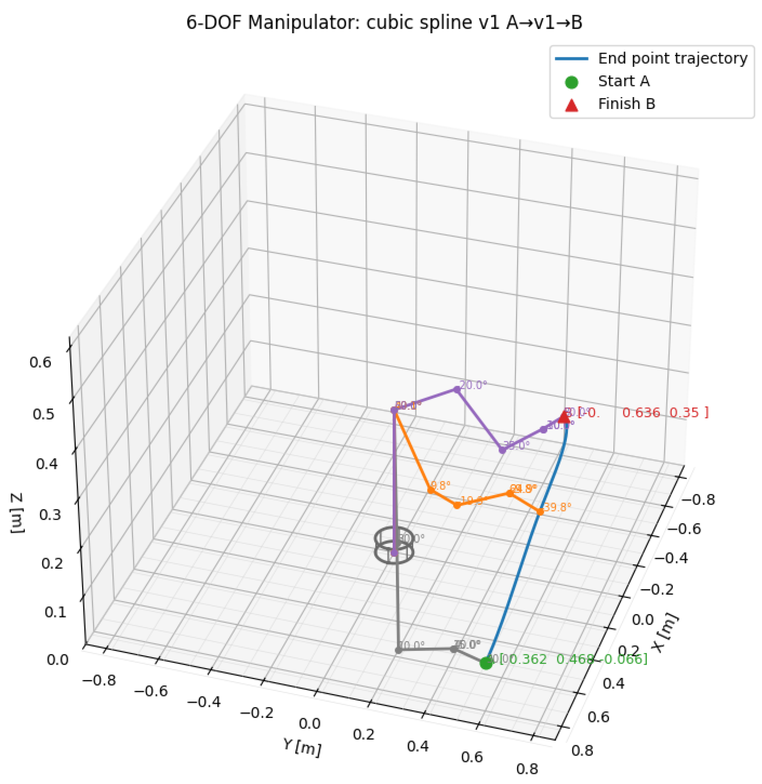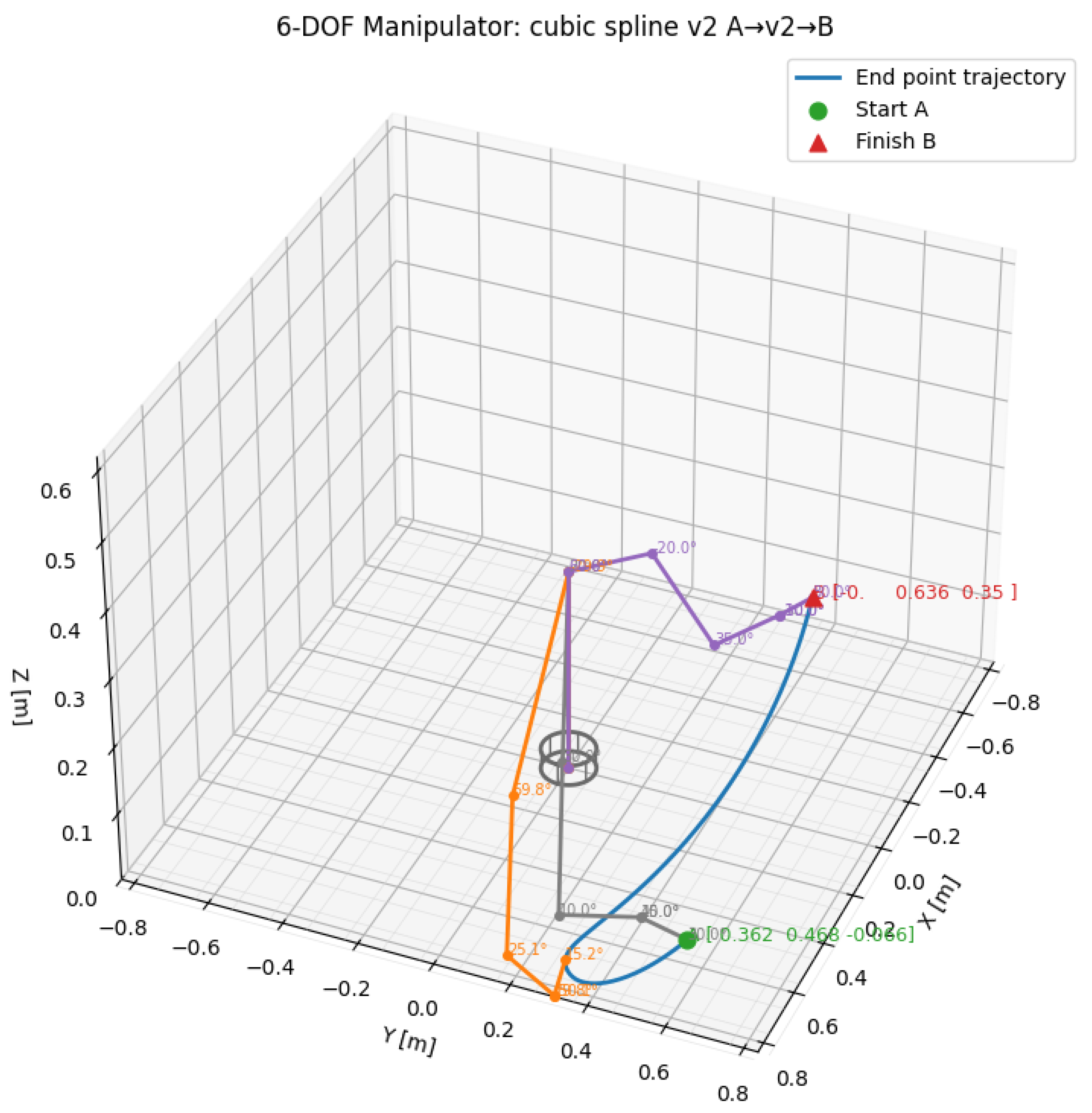The resulting trajectories (although having the same start and end points) can be completely different, due to the different intermediate angles that the joints can have at the intermediate points on the path between the two end points [21]. This can result in curved trajectories in Cartesian space that can be sinuous, longer or shorter, and with steeper or smoother slopes. For example, in Figure 1 and Figure 2, two possible distinct trajectories are presented that the end point of an articulated manipulator can follow to reach the same target points. The manipulator segments are colored differently (purple, orange and gray) capturing 3 different configurations of the manipulator arm in 3 different locations on the trajectories.

Joint movements are used when the path segment doesn’t have to be geometrically constrained in a linear or circular shape. Such constraints are generally imposed by application-specific elements, such as the requirement to follow a certain part outline. Manipulator movement can be generally described mathematically, taking into account manipulator degrees of freedom or end-effector degrees of freedom. For the first case, the workspace of the manipulator is used for movement algorithms, while for the second case, the joint space represents the reference. In the first case, motion planning relies heavily on the inverse kinematics of the manipulator. This means that joint movement, speed, acceleration, etc., are determined by using end-effector movement data as input. Thus, constraints such as speed and acceleration limits for each joint, as well as singularities, must be taken into account. When executing point-to-point movements, since the path itself is not constrained, the most convenient approach is to use the joint space. The focus in this case is on direct kinematics, with only a few elements that require inverse kinematics calculations. Because only the end point of the path is imposed in these situations, the joints will each move in a linear fashion towards the required position, and the end-effector trajectory will be generated as a result of joint movement [22].

Considering the aspects presented above, when working in the joint space, the path itself is not constrained (although there are some limitations to be considered, such as obstacle avoidance); the focus in this case is on choosing the most convenient trajectory. Theoretically, there is an infinite number of possibilities (paths that can be chosen to reach a target point). By establishing certain objectives, the path can be optimized, since its relative flexibility is suitable for modifications. Many applications are using point-to-point movement as the main approach for trajectory generation, mainly in the pick-and-place category [23].

This lack of control over the overall shape of the trajectory makes traditional solutions often suboptimal in applications where cycle time and energy consumption are critical [24]. In this context, the application of the principle of least action represents an opportunity to obtain shorter trajectories. Taking into account that the path length is closely linked to other trajectory parameters and is often influenced by the various optimization algorithms, developing methods of path length reduction can offer the necessary compensation tools. Furthermore, a shorter path length can lead to improvement regarding major aspects of trajectory optimization, such as energy efficiency and component wear. Traditionally, works that do take into account trajectory length are either trying to avoid increasing this parameter or choosing the solution that minimizes the impact.

The purpose of this article is to demonstrate that post-processing of initial trajectories based on this principle can lead to measurable improvements [25]. Also, the study uses a different approach to trajectory optimization, approaching path length as the main focus of the research. The main goal of the paper is to develop a methodology that generates shorter path lengths for point-to-point movement instructions. The generated path is essentially an alternative to joint movement, combining the advantages of shorter distance, lower energy consumption, and lower component wear, without being constrained by a specific geometric configuration (as in the case of linear or circular movement). The study is limited to articulated-arm manipulators with six degrees of freedom. Because the work aims to develop a path generation method that can be generally applied to a wide range of applications, and since the movement is generated in joint space, the loads on the articulated arm of the manipulator are not taken into consideration (also, because the focus of the research is on the kinematics aspects of the manipulator movement.

2. State of the Art

The topic of trajectory planning and optimization, as well as control strategies, has always been of major interest. Significant research efforts are continuously directed towards improvement in these areas. Through a comprehensive review of the literature, Urrea [26] showed that significant advances have been made in industrial robotics regarding control strategies and performance optimizations, citing trajectory and cycle time optimizations as points of major concern. Also, Urrea et. al. [27,28] concluded that advances in industrial robotics are strongly linked to optimization methods and adaptability, including trajectory planning as one of the major approaches.

The geometric trajectory of an articulated manipulator is essentially generated by numerical interpolation between two target points (a starting and a final point). There are two main types of interpolation:

(a)

Interpolation in Cartesian space.

(b)

Interpolation in joint space.

Following linear interpolation in Cartesian space (known as interpolation for MoveL type movements—“move linear”), for each target point that the manipulator must reach, an inverse kinematic (IK) [29] calculation is made to determine the angles required for each joint so that the initial points are reached. The resulting trajectory is perfectly linear, representing the shortest distance between the two target points, and meaning that this type of trajectory cannot be improved in terms of length.

The other method (known as MoveJ interpolation) involves interpolating the positions (angles) of each joint individually. In this case, the number of intermediate points or positions is essential for the shape of the resulting trajectory. To see how the trajectory generation is calculated in this way, we must first establish the following aspects:

• The manipulator has segments chained and connected to each other by n joints.
• There must be at least two known configurations:

  ○

  start: q_start = [q_1,s, q_2,s, …… q_n,s,]

  ○

  finish: q_finish = [q_1,f, q_2,f, …… q_n,f,]

Generating trajectories between two points involves determining the series of intermediate configurations qk that ensure continuous movement between the start and end positions. The calculation method is called “linear interpolation between joint vectors” and is calculated:

$$q\left(s\right)=\left(1-s\right)·q_{start}+q_{finish}, s\in \left[\mathrm{0,1}\right]$$

(1)

$$q\left(s\right)=q_{start}+s{·(q}_{finish}{-q}_{start})$$

(2)

where $q_{start}$ and $q_{finish}$ are the start and end configurations and $s$ is called the interpolation parameter which varies from 0 to 1 and controls the intermediate position on the trajectory.

• At $s=0:q\left(0\right)=q_{start}$—that is, the starting position.
• At $s=1:q\left(10\right)=q_{finish}$—that is, the finish position.

This parameter $s$staggers the trajectory into a number of equal steps (N), for example for N = 20:

$$s_k={\displaystyle \frac{k}{N}},k=\mathrm{0,1},\dots , N$$

(3)

$$s_0=0, s_1={\displaystyle \frac{1}{20}}=0.05, s_2={\displaystyle \frac{2}{20}}=0.1, \dots ...,s_N={\displaystyle \frac{20}{20}}=1$$

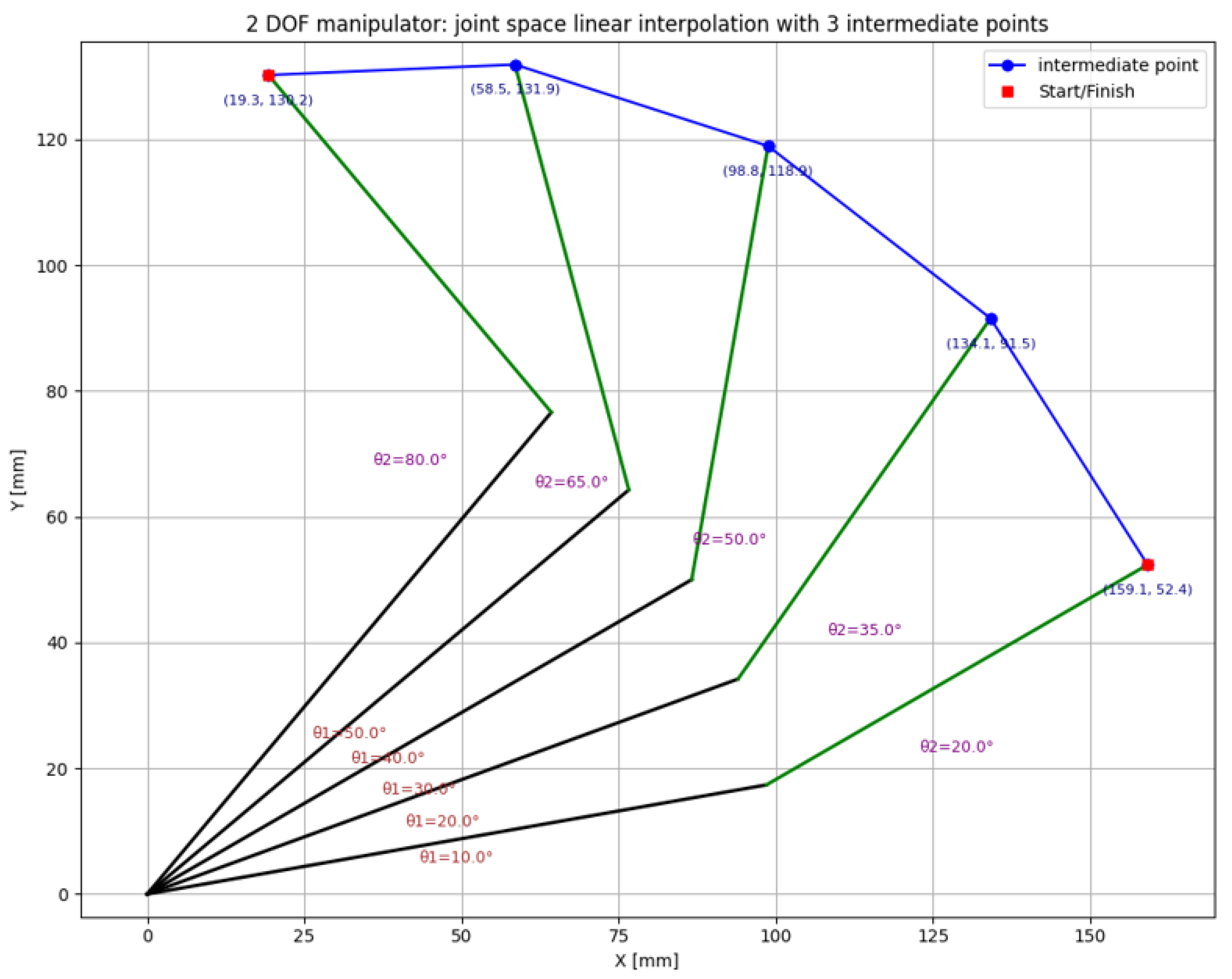
For simplicity, we will consider a manipulator with only two joints with known start and end configurations.: q_start = [10°, 20°], q_finish = [50°, 80°]; and a total number of steps N = 5 (start, intermediate1, intermediate1, intermediate1, finish). We calculate the joint angles for each step:

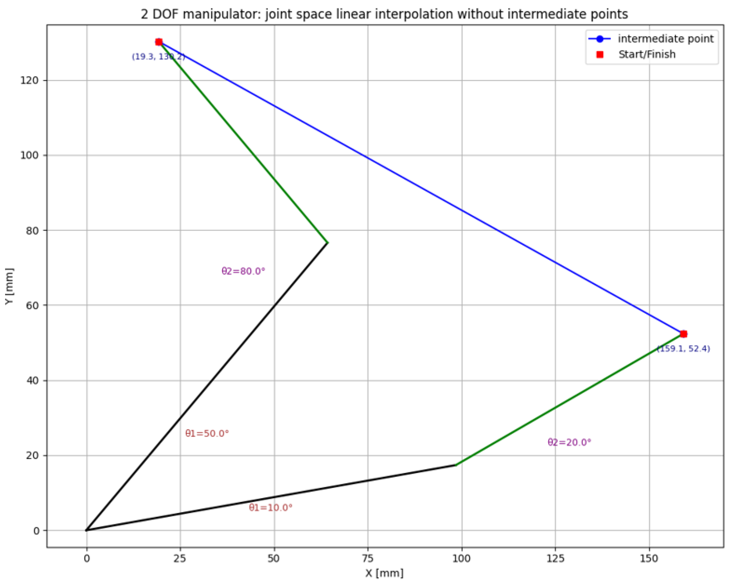
In Figure 3 and Figure 4, the configurations of the joints for movement between two points, without intermediate steps and with 3 intermediate steps (according to the calculation in

Table 1. Calculation of angles of intermediate configurations.

k	${\mathit{s}}_{\mathit{k}}$	j1	J2	${\mathit{q}}_{\mathit{k}}$
0 (start)	$s_0$ = 0	$10+0·(50-10)$ = 10	$20+0·(80-20)$ = 20	[10, 20]
1	$s_1$ = 0	$10+0.25·(50-10)$ = 20	$20+0.25·(80-20)$ = 20	[20, 35]
2	$s_2$ = 0	$10+0.5·(50-10)$ = 30	$20+0.5·(80-20)$ = 20	[30, 50]
3	$s_3$ = 0	$10+0.75·(50-10)$ = 40	$20+0.75·(80-20)$ = 20	[40, 65]
4 (finish)	$s_4$ = 0	$10+1.0·(50-10)$ = 50	$20+1.0·(80-20)$ = 20	[50, 80]

) are graphically represented together with the theoretical trajectories of the manipulator. Trajectory is represented in blue while the manipulator links are represented in black (first link) and green (second link).

In real operation, trajectories that include steep slope variations are to be avoided. These sudden changes in position at nodes cause sudden variations in speeds, accelerations, and torques of the drive motors, which translate into transients and movements with mechanical shocks, vibrations, and positioning errors. We must therefore ensure that the manipulator does not “jump” from one point to another and can follow a trajectory fluently between two target points. Therefore, a major objective in trajectory generation is the smoothing of the trajectories. Such curves can be generated by spline type interpolations (cubic or quintic) [30]. The cubic spline is a function made up of pieces of degree 3 polynomials “glued” together at the nodes so that the function is continuous and has continuous derivatives. This translates into real-world operation in trajectories without corners and without sudden changes in speed and acceleration. The general formula is:

$$S_k\left(x\right)=a_k+b_{k }\left(x-x_k\right)+{c_{k }\left(x-x_k\right)}^2+{d_{k }\left(x-x_k\right)}^3$$

(4)

where: $S_k$ = cubic polynomial; $a_k, b_{k, } c_k, d_k$ = coefficients calculated to respect the continuity and point-to-point conditions, and which are calculated by solving a system of equations starting from:

• $S_k\left(x_k\right)=$$y_k$ (the spline passes through the starting point)
• $S_k\left(x_{k+1}\right)= y_{k+1}$ (the spline passes through the endpoint of the interval)
• ${S\prime }_k\left(x_{k+1}\right)= {S\prime }_{k+1}\left(x_{k+1}\right)$ (ensure speed continuity at nodes)
• ${S”}_k\left(x_{k+1}\right)= {S”}_{k+1}\left(x_{k+1}\right)$ (ensures continuity of acceleration at junctions)
• ${S”}_0\left(x_0\right)=0,{S”}_n\left(x_{n-1}\right)=0$ (the acceleration at the ends is zero)

In total, 4(n − 1) coefficients and the same number of equations will be obtained. From a mathematical point of view, a spline of degree 4 can also be constructed, but even-degree splines are less used in practice because they do not bring any clear additional benefits and tend to have an oscillating behavior called the “Runge Phenomenon” [31]. For this reason, in robotics, the cubic spline is usually used to obtain smooth trajectories or quintic spline if super-smoothness is required. The quintic spline is like the cubic spline except that each piece represents a degree 5 polynomial. The general form is:

$$Q_k\left(x\right)=a_k+b_{k }\left(x-x_k\right)+{c_{k }\left(x-x_k\right)}^2+{d_{k }\left(x-x_k\right)}^3+{e_{k }\left(x-x_k\right)}^4+{f_{k }\left(x-x_k\right)}^5$$

(5)

where this time the coefficients are calculated to respect the continuity conditions inclusive for the 3rd derivative (smooth velocity, acceleration and jerk) [32]. The conditions imposed are several:

• $Q_k\left(x_k\right)=$$y_k$ (the spline passes through the starting point)
• $Q_k\left(x_{k+1}\right)= y_{k+1}$ (the spline passes through the endpoint of the interval)
• ${Q^{\left(j\right)}}_k\left(x_{k+1}\right)= {Q^{\left(j\right)}}_{k+1}\left(x_{k+1}\right)$ (continuity for derivatives 1, 2, 3, 4)
• ${Q\prime \prime \prime }_0\left(x_0\right)=0,{Q\prime \prime \prime }_n\left(x_{n-1}\right)=0$ (3rd derivative at the ends is zero)

The resulting system is larger, comprising 6(n − 1) unknowns and as many equations, and unlike the cubic spline, here the 3rd (“Jerk”) and 4th (“Snap”) derivatives also intervene, which indicate how quickly the acceleration changes and how quickly the jerk changes. In practice, the interpretation of these two parameters is: high-value jerk -> sudden accelerations or decelerations; high-value snap → larger variations of the jerk, making it difficult to control such a mechanical system precisely [33].

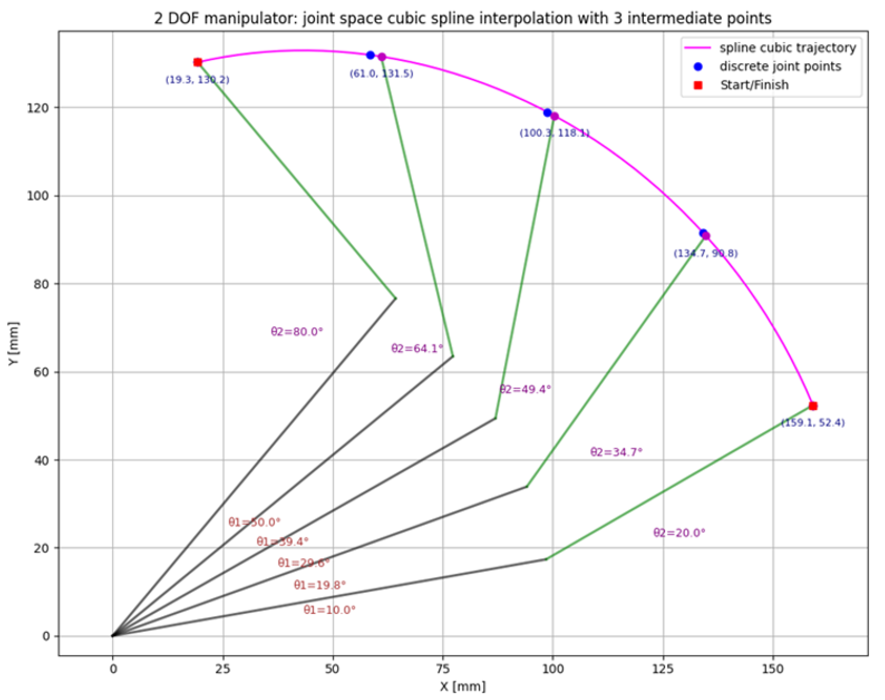
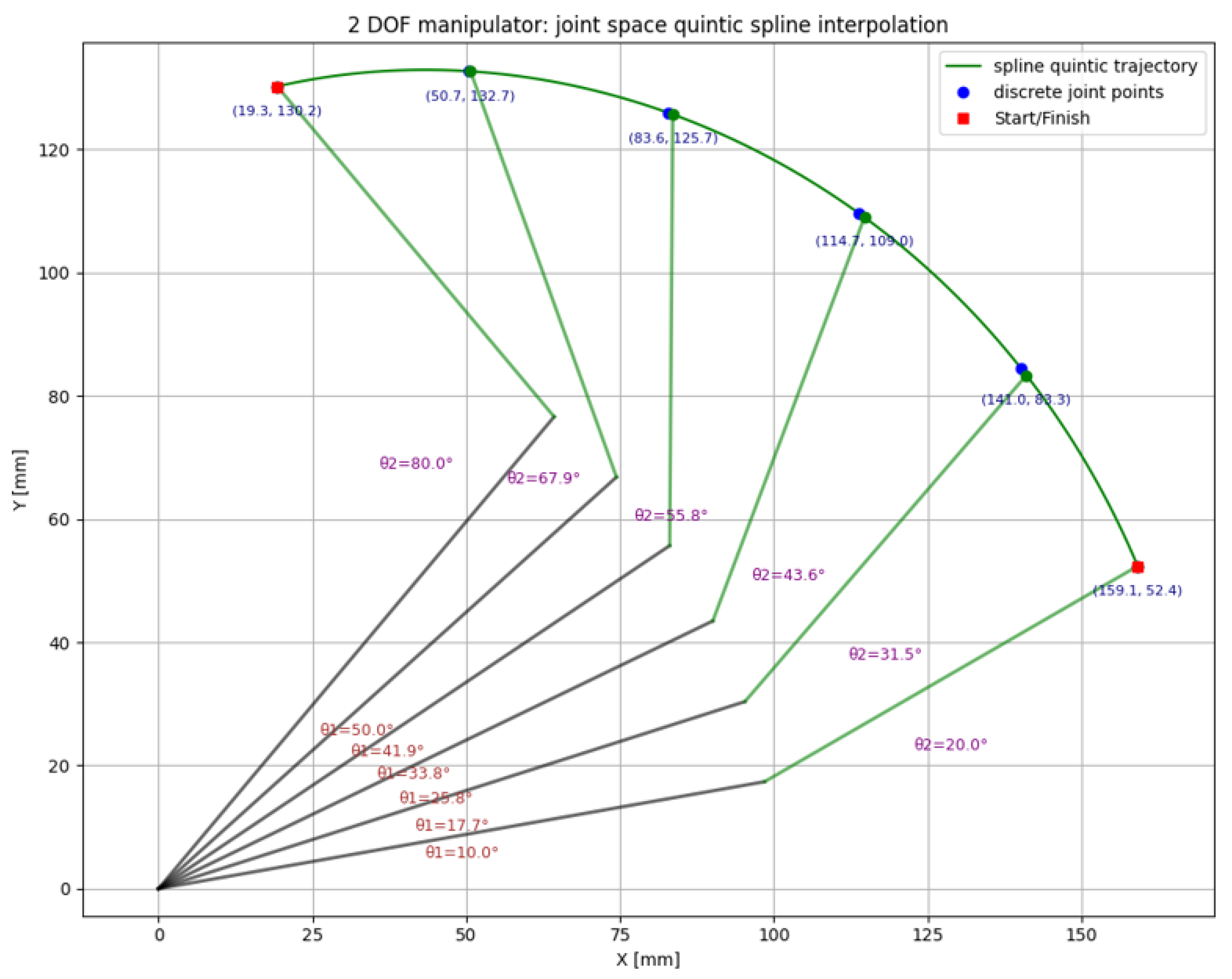
To calculate the joint configurations in intermediate positions by interpolation, a minimum number of 5 points (end, end, and 3 intermediate points) is required for cubic interpolation and a minimum number of 6 points (end, end, and 4 intermediate points) for quintic interpolation. For the simplified case of the 2-degree-of-freedom manipulator, the intermediate joint positions and the trajectories generated by cubic and then quintic interpolation are presented in Figure 5 and Figure 6. Trajectory is represented in purple while the manipulator links are represented in black (first link) and green (second link).

As can be seen from the 2 graphs, the generated trajectories are continuous, with small differences in the intermediate positions calculated between the target points. These differences in the intermediate positions are irrelevant if we are talking about free movements/transitions from one position to another of the manipulator (we excluded from the start the case of linear movements in which the trajectory must be rectilinear, as well as the cases of applications in which the manipulator must follow exactly a pre-established curve). We also specify that, from here on, we will focus on the lengths of the trajectories generated in the classical way, respectively, the attempt to obtain alternative, shorter trajectories applying the principle of minimum action [34].

3. Materials and Methods

Section 3 presents the theoretical mathematical algorithm required to optimize the trajectories using the proposed method. This computational algorithm was also integrated with the help of ChatGPT v5 into a Python 3.13 (64-bit) script that effectively performs the calculations based on input data provided by the user (targets that compose initial trajectories). This calculation file is made available to readers on the GitHub repository (path_optimization_v2 (v1.0.0), GitHub commit 795efb5) specified also under the Data Availability Section. Also, the GenAI tools ChatGPT v5 and Google Translate were used for text translation, reformulating the text in English, as well as for rewriting the abstract and conclusions in a more concise manner.

We consider a set of target points between which the manipulator must execute movements in successive order. These targets are and will remain fixed. We note these targets: q(1), q(2)… q(n); and the s segments of the trajectory that connect 2 consecutive points such that: $q^s\to q^{\left(s+1\right)}$. In Figure 7, three target points are represented, connected by generic trajectory segments.

In order to search for alternative routes for each of the trajectory segments, internal nodes must be created. These internal nodes are intermediate points between the ends of the segment (between successive targets) that will be used to optimize the trajectory segment. A trajectory segment must include at least one intermediate node (K ≥ 1). The greater the number of intermediate nodes, the more solutions for alternative trajectories can be found. We denote the set of internal nodes:

$${\mathit{\chi }}^{\mathit{s}}=\left\{x_1^s,x_2^s\dots .x_K^s,\right\}, x\in R^6 \left(\mathrm{a}\mathrm{n}\mathrm{g}\mathrm{u}\mathrm{l}\mathrm{a}\mathrm{r} \mathrm{v}\mathrm{a}\mathrm{l}\mathrm{u}\mathrm{e}\mathrm{s} \mathrm{o}\mathrm{f} \mathrm{t}\mathrm{h}\mathrm{e} 6 \mathrm{j}\mathrm{o}\mathrm{i}\mathrm{n}\mathrm{t}\mathrm{s}\right)$$

In Figure 8, for each of the initial segments, 2 intermediate nodes were added (K = 2).

Now we have each path segment divided into several pieces. We will call each point that forms these pieces stations. Together with the ends of each segment, the list of stations is:

$$\left[{\mathit{q}}^{\mathit{s}},{\mathit{x}}_1^{\mathit{s}},\dots ,{\mathit{x}}_{\mathit{K}}^{\mathit{s}},{\mathit{q}}^{\mathit{s}+1}\right]$$

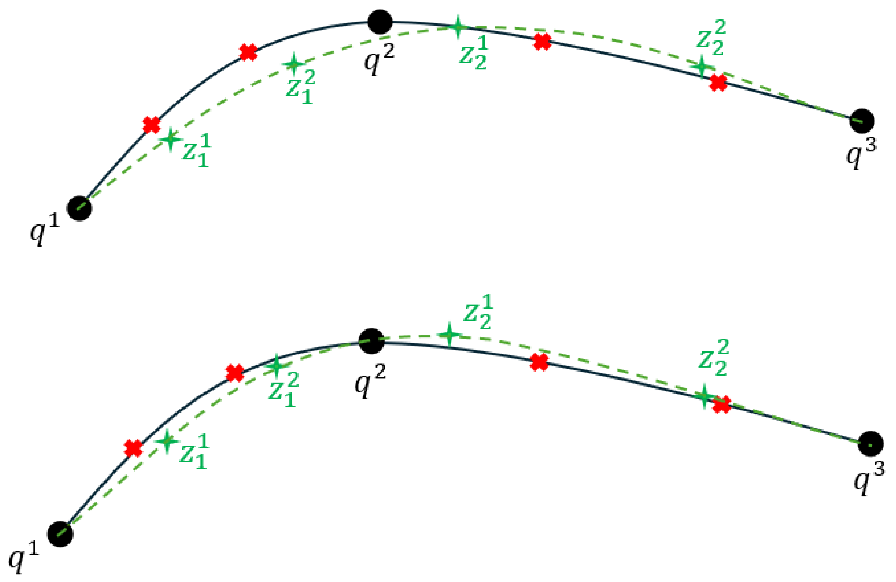
Except for the ends (which coincide with the targets) the position of these stations will be altered iteratively and for the new position of these targets new segments of trajectories will be generated by linear interpolation in joint space, looking for solutions, whose lengths are smaller than the initial one. In other words, it will look for the cost function with the lowest value. In Figure 9, alternative routes obtained between the moved stations (denoted by z) are exemplified where black dots represent initial targets, black lines represent initial trajectory, red crosses represent intermediate nodes on the initial trajectory, green stars represent altered positions of intermediate nodes trough which alternate trajectory (green dots) is constructed.

In our case, the cost function (we will denote it by J) depends on all nodes on all segments and we can write it as follows:

$$\mathit{J}\left(\left\{{\mathit{x}}_{\mathit{j}}^{\mathit{s}}\right\}\right)=\mathit{L}\left(\mathit{P}\right)$$

(6)

where L represents the length and P represents the complete trajectory obtained by concatenating all segments (i.e., the length along the entire path traveled by the manipulator to reach all targets). Recall that the nodes and stations represent configurations of joints (the angles of the manipulator joints are known) and the trajectory in Cartesian space (3D) must be calculated. For this, it is necessary that for each position (p) of the manipulator on the entire path traveled (P) forward kinematics (FK) be applied. Notations:

$$\mathit{P}=\left\{{\mathit{p}}_0,\dots ,{\mathit{p}}_{\mathit{n}}\right\}; {\mathit{p}}_{\mathit{i}}={\mathit{f}}_{\mathit{T}\mathit{C}\mathit{P}}\left({\mathit{z}}_{\mathit{i}}\right)\in {\mathit{R}}^3$$

where f_TCP is the forward kinematics (DH) mapping [35] from the joints to the TCP position (tool center point or manipulator endpoint). With these positions whose Cartesian coordinates are now known, the path length can be measured:

$$\mathit{L}\left(\mathit{P}\right)={\sum }_{\mathit{i}=0}^{\mathit{n}-1}{‖{\mathit{p}}_{\mathit{i}+1}-{\mathit{p}}_{\mathit{i}}‖}_2\left[\mathit{m}\right]$$

(7)

At this point we know the cost function and how we can calculate the lengths of the paths. But to find the minimum of the function J assumes that in an iterative way, at each calculation step, the positions of the stations are modified, and all the calculation steps are completed. Since these modifications are difficult to do manually, a simulated annealing [36] optimizer was implemented that randomly tries to modify the variables (in our case, the joint angles). If we denote the current iteration by t and the total number of iterations set by T, then we can describe how at each iteration t the optimizer generates a Gaussian perturbation [37] with standard deviation:

$$\mathit{\delta }\left(\mathit{t}\right)={\mathit{\delta }}_0+({\mathit{\delta }}_{\mathit{m}\mathit{i}\mathit{n}}-{\mathit{\delta }}_0){\displaystyle \frac{\mathit{t}}{\mathit{T}}}$$

(8)

The perturbation sizes δ are user-defined and represent how much the nodes can move (δ_0) and by what increment these nodes can be moved (δ_min).

At each alteration of the position of the internal nodes, the length of the trajectory must be recalculated. The trajectory is a continuous curve in the articulation space, given by a cubic spline through the target points and the internal nodes adjusted to the optimization, but in order to numerically measure the length in Cartesian space, nothing is interpolated. Each segment is sampled in a number of equidistant pieces (the evaluation density) for which we obtain a vector of joint angles. Knowing the angles of the manipulator in all these, we can calculate by direct kinematics the locations in Cartesian space of the manipulator tip for all these positions. Thus, a polyline is constructed by joining all these successive points. Of course, a polyline generally underestimates the real length of a curve, a chord being shorter than an arc. But to reduce the error, a higher evaluation density can be used so that the “discretization” of the curve is more refined and the calculated results fall within an acceptable margin of error. The measured lengths (which are nothing more than the sum of the chords) are then compared with the reference lengths obtained by cubic spline interpolation. The solutions thus identified can be better or worse and need to be evaluated in some way. For this reason, a form of regularization is needed so that ugly shapes/large oscillations in the joint space between the ends and nodes can be penalized to ensure that the obtained solutions are as smooth as possible. So, the objective function to be minimized becomes:

$$\mathit{J}\left(\left\{{\mathit{x}}_{\mathit{j}}^{\mathit{s}}\right\}\right)=\mathit{L}\left(\mathit{P}\right)+{\mathit{C}}_{\mathit{r}\mathit{e}\mathit{g}}\mathit{R}$$

(9)

where C_reg is a regularization coefficient (usually very small values 10e⁻⁶…10e⁻⁵) by which we determine what importance/weight we assign to this regularization and R is the total regularization function in the joint space. The regularization on each trajectory segment is determined by calculating the sum of the squares of the differences between each two consecutive stations.

$${\mathit{R}}^{\mathit{s}}={\sum }_{\mathit{i}=0}^{\mathit{K}}{‖{\mathit{z}}_{\mathit{j}+1}^{\mathit{s}}-{\mathit{z}}_{\mathit{j}}^{\mathit{s}}‖}_2^2$$

(10)

At this point, if two objective functions J have the same length, the solution with the smallest regularization will be considered the best. To more intuitively illustrate how this calculation process can be utilized, a concrete case study is exemplified in the following chapter.

4. Case Study

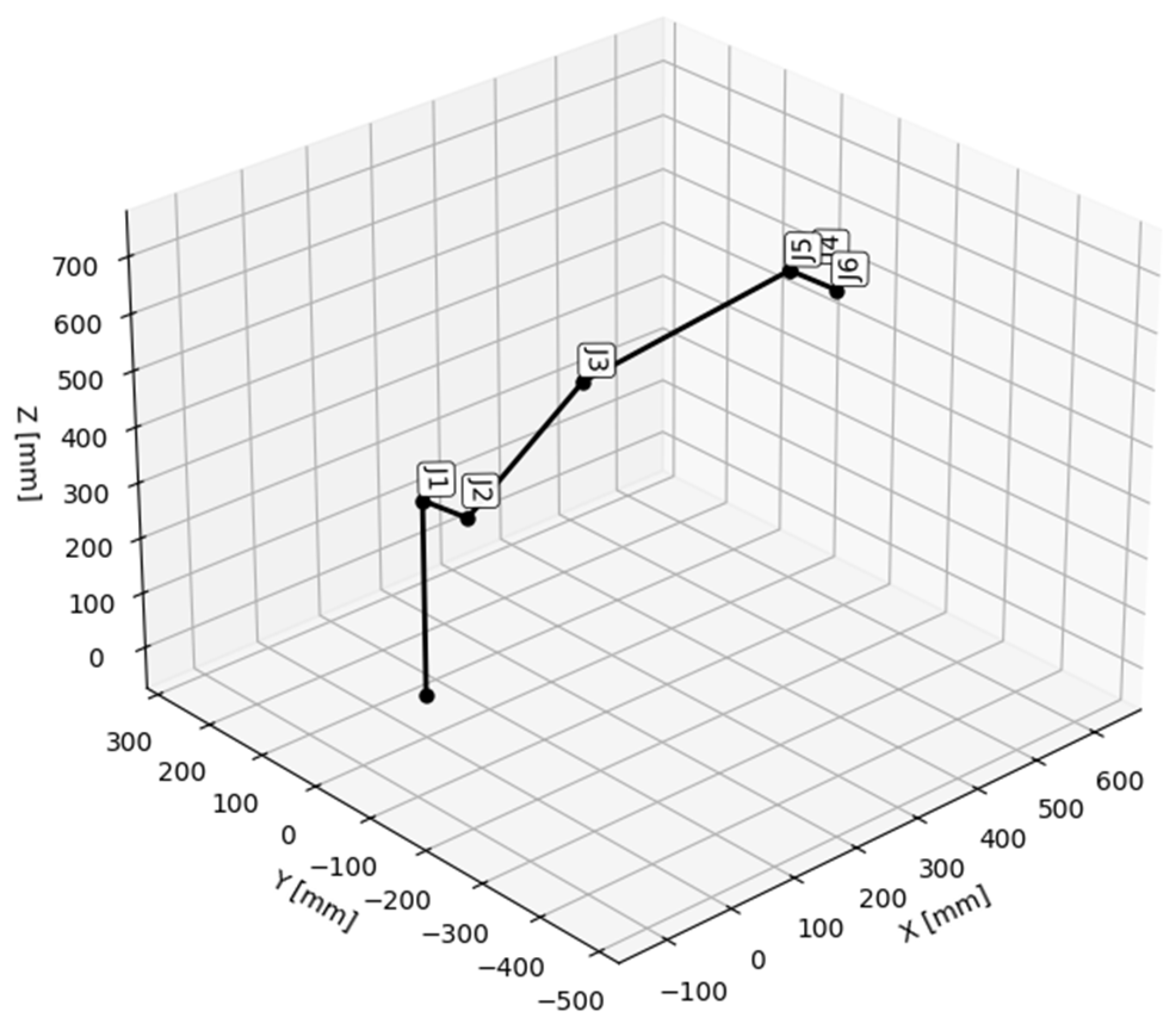
We consider the case of a real manipulator with 6 degrees of freedom (ABB IRB140 model) whose kinematic scheme and dimensions are described by the Denavit-Hartenberg parameters in

Table 2. Geometric parameters of the manipulator.

	J1	J2	J3	J4	J5	J6
α [°]	0	−90	0	−90	90	−90
a [mm]	0	70	360	0	0	0
d [mm]	352	0	0	380	0	65
θ [°]	0	−90	0	0	0	180

. These parameters represent the initial positions of the joints and the lengths of the manipulator segments. The structure of this manipulator is presented in Figure 10.

4.1. Trajectories Between a Single Set of Points: Checking the Convergence of Path Lengths and Test Run

For the presented manipulator, we will generate the trajectories between 10 target points defined randomly in the workspace. The trajectories between the points will first be generated both by the classical cubic spline interpolation solutions and by quintic spline interpolation. Finally, the optimized trajectories will be generated by applying the principle of minimum action (complete methodology described in the previous chapter) with the objective of shortening the lengths of the trajectories. In

Table 3. Target points used for trajectory generation.

	X [mm]	Y [mm]	Z [mm]	Rx [°]	Ry [°]	Rz [°]
1	90.405	−12.224	44.548	63.158	−97.397	332.936
2	86.176	57.213	−86.94	−15.876	−31.008	298.735
3	47.475	64.552	−30.185	−87.284	13.1	−305.328
4	108.118	26.333	26.456	−46.552	112.968	275.185
5	91.867	−61.072	−25.99	−145.983	−82.971	128.134
6	80.772	93.502	−51.351	−41.453	−7.307	−217.37
7	−122.126	−4.859	−69.156	54.34	−15.084	232.875
8	66.087	−37.527	39.807	97.525	−27.005	−148.17
9	60.224	−72.05	−74.017	−157.644	68.862	115.396
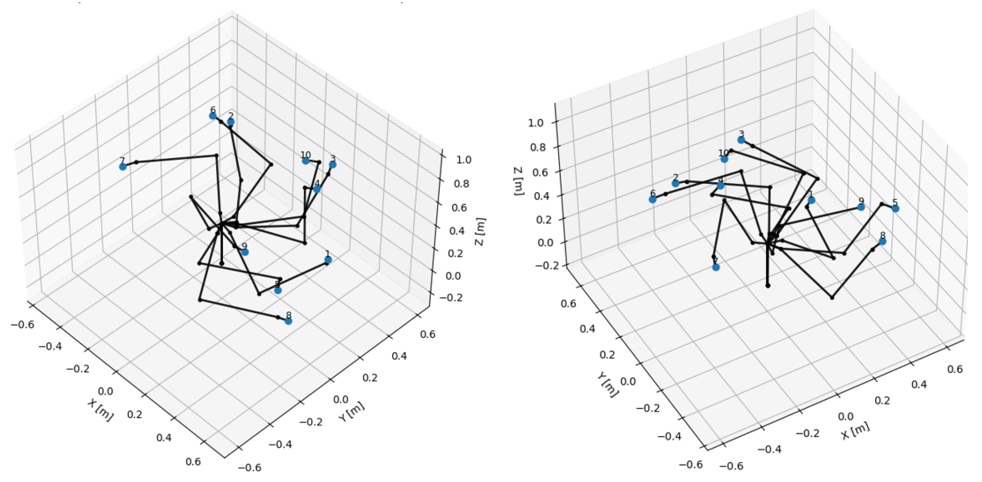
10	67.705	56.146	−27.395	21.997	−86.449	−269.829

, the 10 target points are presented, where X, Y, and Z represent the Cartesian coordinates of the point and Rx, Ry, and Rz represent the angles that determine the orientation of the targets. These target points are represented in Figure 11 in the manipulator workspace together with the manipulator configurations necessary to reach them.

The measurement of the path lengths depends very much on the density of the points on the curve used for the evaluation. Considering that we only want to optimize the paths that the robot has to follow in free movement, and the lengths of these paths are in the tens of cm range, we set a threshold of ≤1 mm in the application. An initial test was run to ensure that the number of evaluation points is large enough to ensure convergence of all paths (cubic, quintic, and optimized) with a difference of less than 1 mm. The results of the convergence test can be observed in

Table 4. Convergence of path lengths.

Traj. Type	Eval Density	Length [m]	Difference from Last [mm]	≤Threshold?
optimized	80	10.5510904	start desity
optimized	160	10.55109169	0.001281257	YES
optimized	320	10.55109201	0.000320314	YES
optimized	640	10.55109209	8.01 × −105	YES
cubic	80	11.1235568	start desity
cubic	160	11.12468944	1.132642826	NO
cubic	320	11.12497264	0.283197502	YES
cubic	640	11.12504344	0.070801961	YES
quintic	80	11.81747855	start desity
quintic	160	11.8187751	1.296552822	NO
quintic	320	11.81909931	0.324207595	YES
quintic	640	11.81918036	0.081055981	YES

. We can see that the trajectory length approximation with any number of evaluation points greater than 320 will generate results with errors less than 1 mm. In all of the further tests, a total of 320 evaluation points were used.

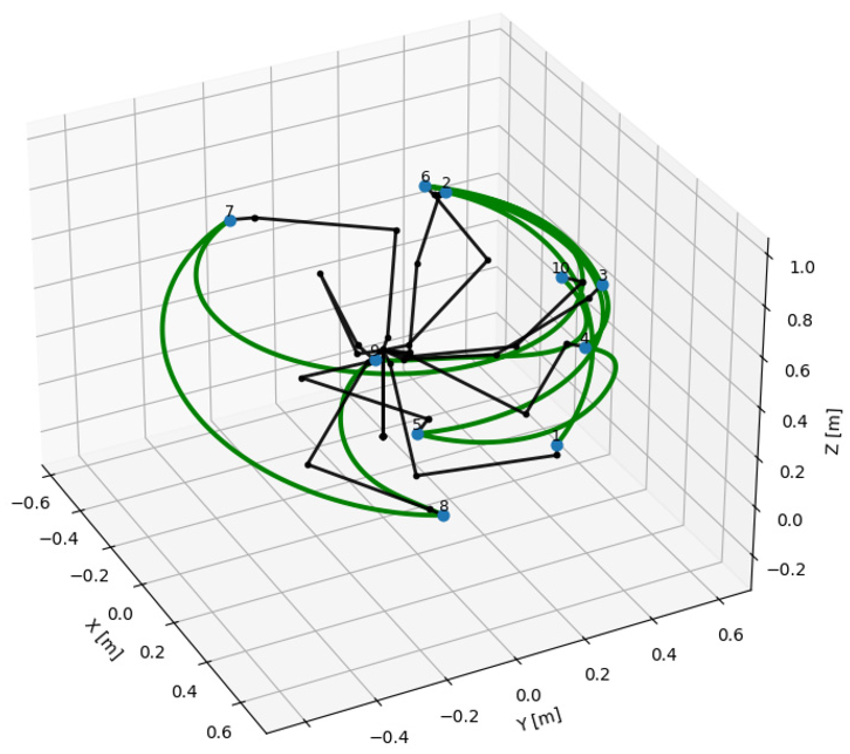
For the 10 targets, the trajectories are generated so that they are traversed in order, from P1 to P2, from P2 to P3, etc., resulting in a total of 9 curves connecting the 10 points. Figure 12 shows the manipulator trajectories generated by cubic spline interpolation (orange curves). Figure 13 shows the manipulator trajectories generated by quintic spline interpolation (purple curves) and Figure 14 shows the trajectories obtained by applying the optimization principle (green curves) presented in the previous chapter. Blue dots that are numbered represent initial target points and black lines represent the manipulator segments in different configurations to reach target points.

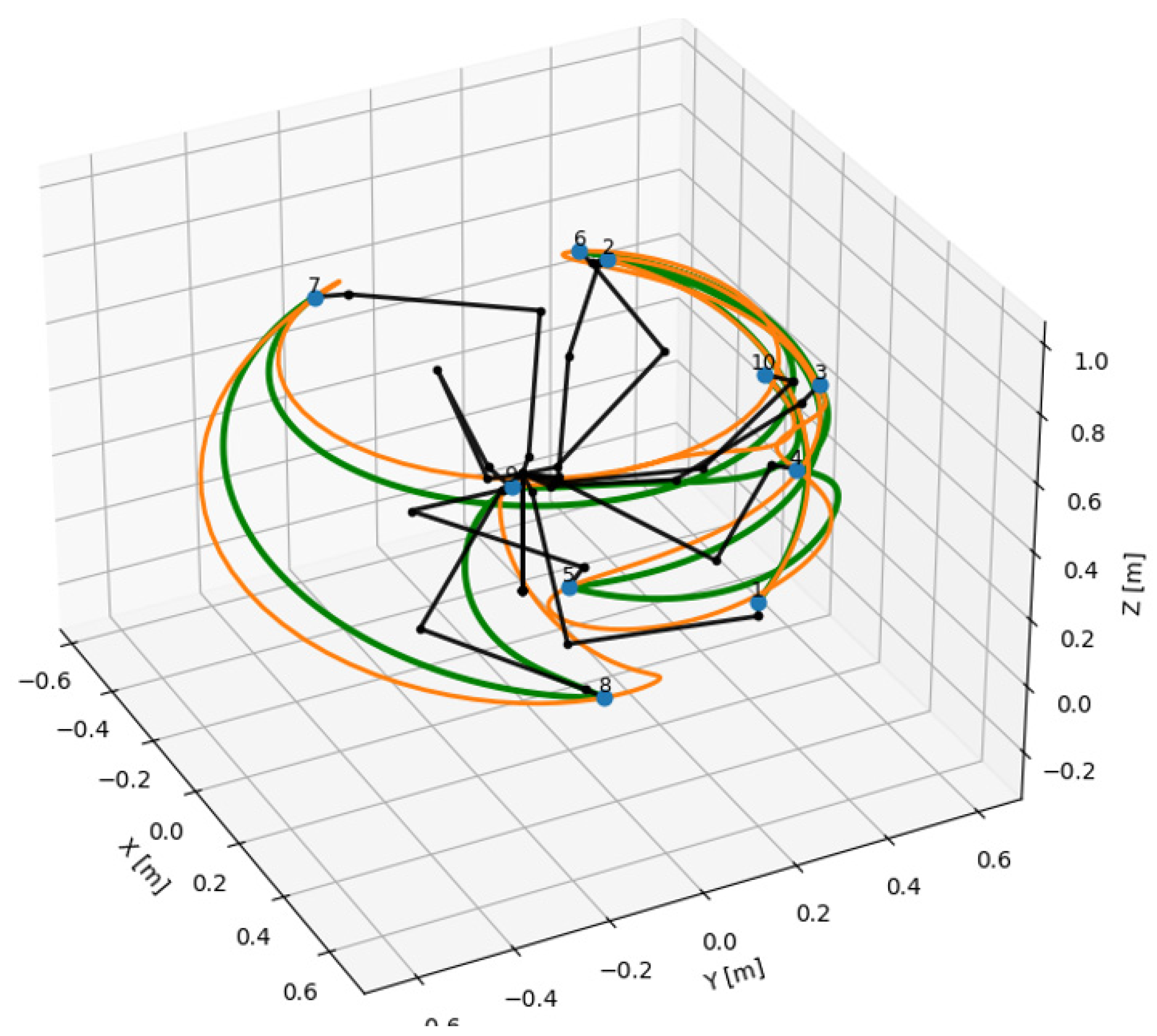
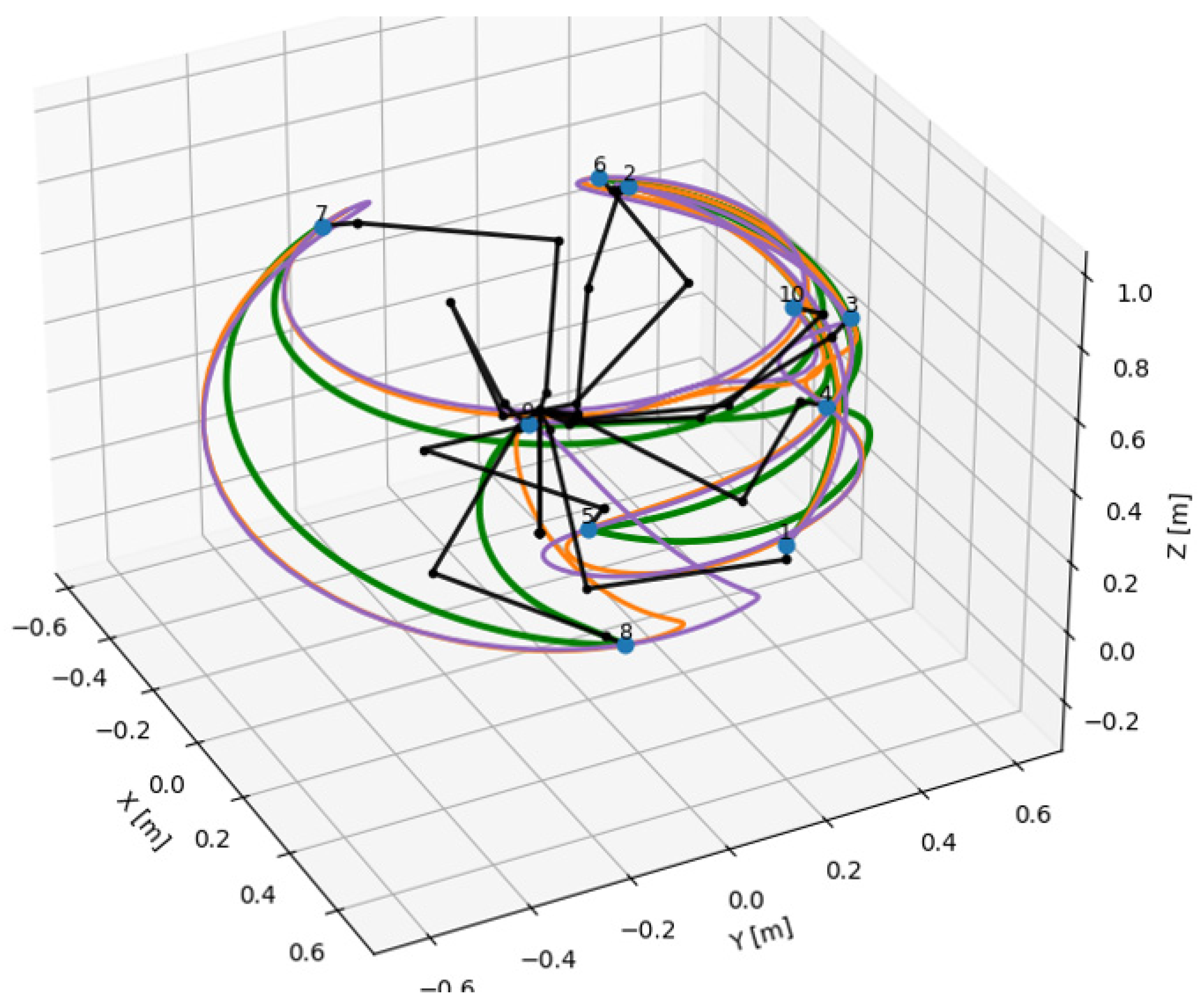
Since the shape of these trajectories is similar and the differences between them are very difficult to observe, these trajectories are presented in superimposed mode in Figure 15, Figure 16 and Figure 17. In Figure 15, the cubic trajectories (orange) are presented superimposed on the optimized trajectories (green), in Figure 16, the quintic trajectories (purple) are presented superimposed on the optimized trajectories (green), and in Figure 17, all 3 types of trajectories are presented simultaneously. In all three figures initial targets points are represented with blue dots numbered from 1 to 10 and manipulator segments are represented in black lines in different configurations to reach target points.

Visualizing the trajectories in graphical form offers the possibility of a quick qualitative assessment, and the first observation that we can draw is that we do not observe any aberrant trajectories. We also notice that the trajectories have similar features but with noticeable differences, which indicates to us, at least on individual segments of the trajectory, that the lengths traveled are also different. For a quantitative assessment of these differences, the metrics of these trajectories are presented in tabular form in Section 5.

At this point, it’s worth noting that, for a specific application, trajectory planning and analysis should take into account aspects such as speed limitations, maximum accelerations, and torque constraints, as well as singularities. However, this is not the case with the current study. Since the goal of the research is to provide shorter paths between trajectory configuration points, this itself implies that the scope of the work is limited to optimizing the joint-type movements. Thus, linear interpolation movements do not fall within the scope of the study—such an improvement wouldn’t be possible for linear interpolation anyway, as linear trajectories are uniquely determined and already represent the shortest path between two points. Since singularity cases for the most common robot structures are well known, and (at least for serial manipulators) are closely linked to linear movements, these kinematic limitations do not apply to point-to-point movements. It should also be noted that, in joint space, the movement is described mathematically by the direct position and velocity kinematics, which determine the end-effector position, orientation, and speed based on individual joints’ movement. Thus, it is the individual joints’ movement that dictates the trajectory parameters, and, therefore, the characteristics of the end-effector movement do not impose any constraints on joint movement. Regarding torque-related constraints, this is heavily dependent on the specifics of the application and operations that are performed by the robot, including the payload. Since the study provides a general framework for optimizing the path length in point-to-point type movements, it does not include specific elements for certain applications.

4.2. Different Configurations and Trajectories Between Multiple Target Point Sets

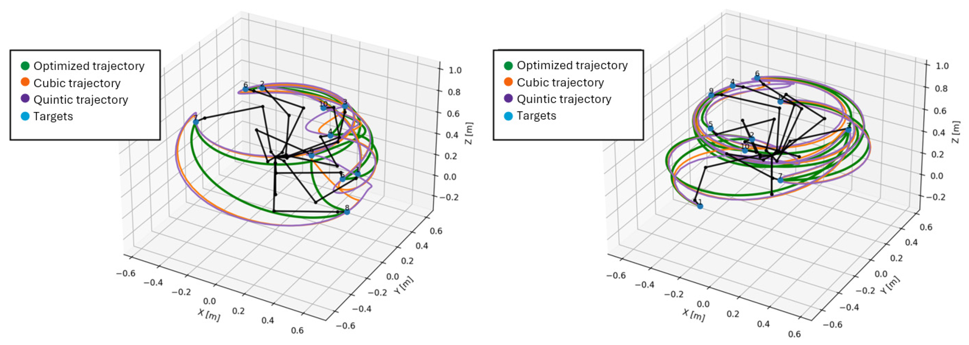
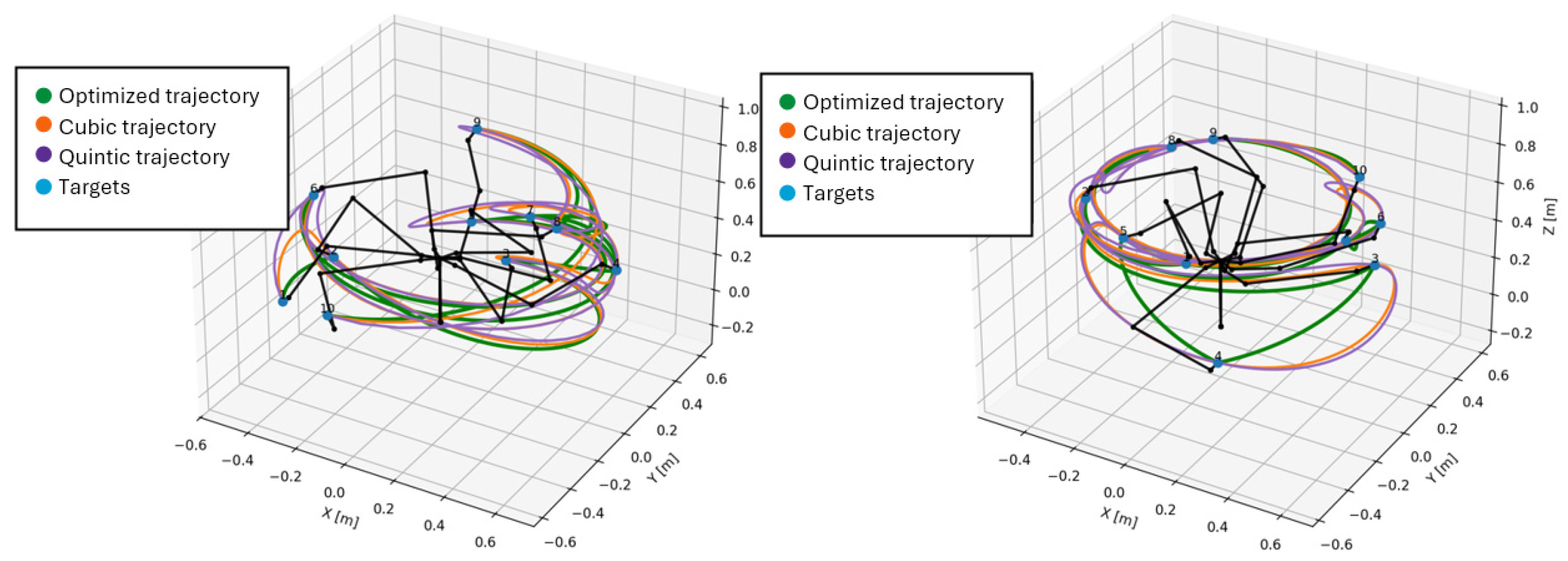
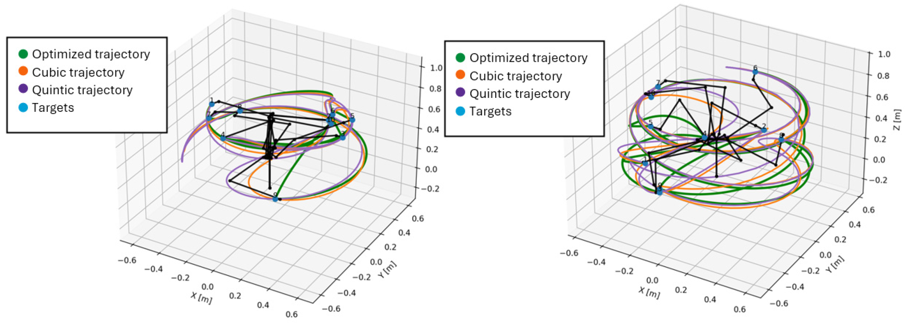
In this scenario, the application was analyzed on sets of points so that we could also obtain some statistical metrics. In the input file, 10 sets of 10 target points each were generated. The first set of 10 points was kept identical to the one from the previous subchapter. The other 9 sets contain completely different target points generated randomly. Due to the very large number of trajectories obtained, the following figures present the overlapping variants (cubic, quintic, and optimized) for each of the 10 sets covered in this scenario (shown in Figure 18, Figure 19, Figure 20, Figure 21 and Figure 22). Same color code is used as in previous figures: cubic trajectory is in orange color, quintic trajectory is in purple color and optimized trajectory is in green color. Initial target points numbered and marked with blue dots.

In this second scenario, we can also see that the optimized trajectories obtained for each set of points are similar to those obtained by cubic or quintic spline interpolation, but for a quantitative assessment, the numerical metrics for all these sets are presented in tabular form in the next chapter.

5. Results

We recall that the method used is an iterative one and that the input parameters for the calculation are: the initial targets (N), the number of intermediate nodes/stations on each segment (z), the maximum value of the displacement of the intermediate nodes (δ_0), the minimum value of the displacement of the intermediate nodes (δ_0), the regularization coefficient (Creg) and the number of iterations. For both presented study cases, the same values of the initial parameters were used and presented in

Table 5. Parameters used for optimization.

Parameter	Value
N	10
z	20
${\delta }_0$ [deg]	5
${\delta }_{min}$ [deg]	0.1
Creg	1 × 10−6
evaluation density	320
i	100

.

In the 100 iterations, the cost functions were calculated and compared with the lengths of the trajectories calculated by cubic and quintic interpolation (whose lengths were calculated by segments and are presented in

Table 6. Lengths of the segments of the cubic trajectory.

Segment	Length [m]
1	1.035585
2	0.578767
$3$	0.489022
$4$	1.226762
5	1.687858
6	2.444982
7	1.833593
8	0.821047
9	1.007427
Total	11.12504

and

Table 7. The lengths of the quintic trajectory segments.

Segment	Length [m]
1	1.105633
2	0.611182
$3$	0.635938
$4$	1.299501
5	1.721185
6	2.428636
7	1.958136
8	1.013572
9	1.045397
Total	11.81918

).

5.1. Results for Single Set of Points

Among the 100 iterations, the candidate solutions were separated by comparing the calculated cost function with the length of the cubic trajectory (from the calculations, this resulted in a shorter length than the quintic one).

Table 8. Values computed for the first 10 iterations.

Iter.	δ [deg]	J Cost	Length [m]	Regularization Penalty	Shorter?
0	5	10.55111891	10.55109209	2.68 × 10−5	YES
1	4.951	20.874362	20.87431911	4.29 × 10−5	NO
2	4.902	20.59416476	20.59412121	4.35 × 10−5	NO
3	4.853	20.73207527	20.73203164	4.36 × 10−5	NO
4	4.804	19.02656266	19.02652185	4.08 × 10−5	NO
5	4.755	18.42859246	18.42855141	4.11 × 10−5	NO
6	4.706	20.10816589	20.10812318	4.27 × 10−5	NO
7	4.657	18.9695764	18.96953525	4.12 × 10−5	NO
8	4.608	17.12315377	17.12311345	4.03 × 10−5	NO
9	4.559	18.83671159	18.83666954	4.21 × 10−5	NO
10	4.51	18.2675479	18.2675072	4.07 × 10−5	NO

presents the calculated values for the first 10 iterations.

A total of 22 solutions were identified that resulted in total path lengths lower than the cubic one. These solutions are presented in

Table 9. The 22 identified solutions that result in total path lengths lower than the cubic one.

Iter.	δ [deg]	J_Cost	Length [m]	Regularization Penalty	Shorter?
0	5	10.55111891	10.55109209	2.68 × 10−5	YES
79	1.129	11.01004046	11.01001281	2.76 × 10−5	YES
81	1.031	11.00981459	11.00978706	2.75 × 10−5	YES
82	0.982	11.12483992	11.12481242	2.75 × 10−5	YES
83	0.933	10.89368873	10.8936614	2.73 × 10−5	YES
84	0.884	10.96554261	10.9655153	2.73 × 10−5	YES
85	0.835	10.91694049	10.9169132	2.73 × 10−5	YES
86	0.786	10.7937389	10.79371167	2.72 × 10−5	YES
87	0.737	10.77945494	10.77942779	2.72 × 10−5	YES
88	0.688	10.75692961	10.75690248	2.71 × 10−5	YES
89	0.639	10.73766958	10.73764249	2.71 × 10−5	YES
90	0.59	10.71161599	10.71158893	2.71 × 10−5	YES
91	0.541	10.69934001	10.69931298	2.70 × 10−5	YES
92	0.492	10.64037586	10.64034888	2.70 × 10−5	YES
93	0.443	10.64243317	10.64240622	2.70 × 10−5	YES
94	0.394	10.63235991	10.63233298	2.69 × 10−5	YES
95	0.345	10.60357656	10.60354967	2.69 × 10−5	YES
96	0.296	10.59670771	10.59668084	2.69 × 10−5	YES
97	0.247	10.57790245	10.57787558	2.69 × 10−5	YES
98	0.198	10.57525813	10.57523129	2.68 × 10−5	YES
99	0.149	10.56273201	10.56270517	2.68 × 10−5	YES
100	0.1	10.55377991	10.55375308	2.68 × 10−5	YES

.

We can see in the table presented that among the candidate solutions, the shortest path length was obtained at the very first iteration when the value of δ was maximum, so the intermediate nodes were moved by the largest magnitude. A centralized comparison of the calculated length values on each segment of the paths is presented in

Table 10. Length comparison by each trajectory segment.

	Trajectory Segments Length [m]
Type	s1	s2	s3	s4	s5	s6	s7	s8	s9	TOTAL
Cubic	1.036	0.579	0.489	1.227	1.688	2.445	1.834	0.821	1.007	11.125
Quintic	1.106	0.611	0.636	1.3	1.721	2.429	1.958	1.014	1.045	11.819
Optimized	1.036	0.564	0.362	1.136	1.596	2.56	1.513	0.739	1.045	10.551

.

The values from the table were colored green, orange, and red to highlight the best, intermediate, and worst results. Given that our objective is global and evaluates only the total length on the entire trajectory and not on each segment, a local increase on some segments may pass the analysis if, however, on other segments the optimization is good enough to compensate and the total length is smaller. This is a compromise that we assume by which we try to obtain a better global result that improves the overall efficiency. Although the optimization method did not provide the best solutions on every single segment of the trajectory, it still found better solutions, so that the global result in this case was considerably smaller.

After this test case with only 10 targets, the batch mode was executed. The same parameters were used except for the input file. The input file for this lot mode contains 10 sets, each containing 10 targets. For each set, global trajectory metrics are presented (individual metrics for each segment can be found in the original results files in the repository), including this time the computing duration for each trajectory type. The optimization method seems to take much longer for given parameters (multiple minutes) than cubic and quintic interpolation (fractions of seconds), thus in the following

Table 11. Trajectory metrics comparison.

	Cubic		Quintic		Optimized		Length Difference [m]
Set	Length [m]	Duration [s]	Length [m]	Duration [s]	Length [m]	Duration [min]	Opt-Cub	Opt-Quin
1	11.125	0.545	11.818	0.549	10.551	36.7	−0.574	−1.267
2	15.844	0.550	17.22	0.621	15.003	37.01	−0.841	−2.217
3	10.21	0.554	10.898	0.543	9.739	37.13	−0.471	−1.159
4	13.471	0.542	14.783	0.569	12.464	37.16	−1.007	−2.319
5	14.789	0.528	15.377	0.554	14.052	37.26	−0.737	−1.325
6	9.996	0.528	11.049	0.552	9.066	37.15	−0.93	−1.983
7	13.879	0.588	14.833	0.541	13.011	37.36	−0.868	−1.822
8	11.748	0.509	13.013	0.565	9.86	37.01	−1.888	−3.153
9	9.675	0.596	10.180	0.519	8.429	37.3	−1.246	−1.751
10	16.800	0.480	17.828	0.501	16.588	38.88	−0.212	−1.24

, computation duration is given in seconds for cubic and quintic splines and in minutes for optimized trajectories.

5.2. Results for Multiple Sets of Points

We can treat the trajectories calculated for multiple sets of points individually (as previously presented in Table 11), or we could even consider a scenario where, in the manipulator work cycle, all target points have to be traversed, so, from the point of view of lengths, it is appropriate to sum and average these values. In continuation of

Table 12. Total lengths and total computation duration.

		Total	Average	Geometric Mean
Cubic	Length [m]	127.537	12.754	12.525
	Duration [s]	5.420	0.542	0.541
Quintic	Length [m]	136.999	13.700	13.460
	Duration [s]	5.514	0.551	0.551
Optimized	Length [m]	118.763	11.876	11.595
	Duration [s]	372.960	37.296	37.292
Length difference	Opt-Cub [m]	−8.774	−0.877	0.764
	Opt-Quin [m]	−18.236	−1.824	1.735

, the total lengths, the total calculation times for generating the trajectories, and the differences/improvements obtained are presented. Also, the average and geometric mean values are calculated.

Therefore, the sum of the lengths of all trajectories generated by cubic interpolation is approximately 127.5 m, and that generated by quintic interpolation is approximately 137 m. Compared to these two cases, the calculated optimized trajectories have a total length of approximately 119 m, which represents a percentage reduction of 6.88% compared to cubic trajectories and 13.31% compared to quintic trajectories.

From the point of view of computational time durations, the optimization process takes much longer (approximately 37 min for each set containing 10 target points, resulting in trajectories with lengths of approximately 12 m) compared to only fractions of a second for cubic and quintic interpolations. But this computational time is irrelevant in the context of the work in which the goal is offline post-processing of pre-existing trajectories, so that it does not imply downtimes for the manipulator.

In terms of path length of mechanical manipulators, a reduction of path length with more than 6% mm is a significant reduction. This means significant path lengths (≥0.5 m for paths generated using 10 target points or ≥8 m for paths generated using 10 different sets of 10 target points each), considering that they operate in most cases in continuously repetitive cycles.

6. Conclusions

This paper has proposed and validated a trajectory optimization method for articulated manipulators based on the principle of least action. By introducing intermediate nodes and iteratively displacing them using a simulated annealing approach, the method enables the identification of alternative trajectories shorter than those obtained with conventional cubic or quintic spline interpolation.

Two case studies were conducted on a 6-DOF manipulator. The first case study conducted on only 10 target points has demonstrated that the optimized trajectories can achieve a reduction in path length of more than 500 mm compared to standard spline solutions. The second case study was conducted on 10 sets containing 10 distinct points each. This was done specifically to be able to extract some statistical data. This time, the total lengths of the trajectories were analyzed and compared, and the results showed improvements of approximately 7–13% meaning reduced travel distances between 8 and 18 m (the total lengths of the cubic and quintic trajectories being between 127 m and 136 m).

Such improvements are particularly significant in industrial contexts, where manipulators operate in repetitive cycles, and even small reductions in trajectory length can accumulate into substantial savings in terms of cycle time, energy consumption, and mechanical wear.

The results also show that the proposed optimization does not generate irregular or impractical paths but instead produces smooth trajectories that respect kinematic continuity. While the method does not guarantee improvement on every single trajectory segment, the overall path optimization proves to be consistently advantageous.

Future work will focus on extending the proposed approach to multi-objective optimization, integrating additional criteria such as smoothness (curvature-based), dynamic constraints (velocity, acceleration, jerk), and energy-based metrics. Moreover, the scalability of the method will be tested in real-time applications, with direct implementation in robot controllers for industrial processes.