Abstract
Computer viruses remain a persistent technological challenge in information security. They require mathematical frameworks that realistically capture their propagation in digital networks. Classical continuous-time, integer-order models often overlook two key aspects of cyber environments: their inherently discrete nature and the memory-dependent effects of networked interactions. In this work, we introduce a fractional-order discrete computer virus (FDCV) model, derived from a three-dimensional continuous integer-order formulation and reformulated into a two-dimensional fractional discrete framework. We analyze its rich dynamical behaviors under both commensurate and incommensurate fractional orders. Leveraging a comprehensive toolbox including bifurcation diagrams, Lyapunov spectra, phase portraits, the 0–1 test for chaos, spectral entropy, and complexity measures, we demonstrate that the FDCV system exhibits persistent chaos and high dynamical complexity across broad parameter regimes. Our findings reveal that fractional-order discrete models not only enhance the dynamical richness compared to integer-order counterparts but also provide a more realistic representation of malware propagation. These insights advance the theoretical study of fractional discrete systems, supporting the development of potential technologies for cybersecurity modeling, detection, and prevention strategies.
1. Introduction
The rapid spread of computer viruses remains a major challenge to cybersecurity, as infections can disrupt critical infrastructures and cause significant economic losses [1,2]. To better understand and predict such propagation, mathematical modeling has been widely employed, often drawing inspiration from epidemiological models [3,4]. While these approaches have provided useful insights, most classical computer virus models are formulated as continuous-time systems with integer-order derivatives. Such formulations may overlook two essential aspects of digital environments: their inherently discrete nature and the memory-dependent interactions within networks [5,6].
In recent years, fractional discrete-time systems have attracted significant attention due to their ability to describe complex processes with memory and hereditary effects while capturing the inherently discrete nature of many real-world phenomena [7,8]. Unlike classical integer-order difference equations, fractional difference equations extend the concept of differentiation and summation to non-integer orders, thereby offering a more flexible framework for modeling dynamical systems. This generalization has been shown to produce richer dynamics, including long-range memory effects, anomalous diffusion, and persistent chaotic behavior, which cannot be observed in the integer-order case [9].
Fractional discrete systems have been applied in various fields, including population dynamics, economic and financial modeling, epidemic spread, image processing, secure communications, and digital technologies [10]. Their ability to combine discrete-time evolution with fractional-order memory makes them particularly suitable for digital environments, where processes evolve in steps but are influenced by past states over long horizons. Moreover, recent studies have demonstrated that fractional discrete systems often exhibit complex and chaotic attractors, which are essential for understanding nonlinear behaviors and for practical applications such as encryption, network security, and emerging technologies [11,12].
Building on these advances, researchers have recently begun exploring the role of fractional discrete models in the study of cyber-epidemics [13,14]. Fractional calculus provides the ability to incorporate long-term memory into the infection process, while the discrete framework naturally reflects the stepwise nature of digital communications, malware propagation, and evolving technologies [15,16]. Despite their potential, however, the development and analysis of fractional discrete computer virus models remain relatively limited compared to their continuous counterparts.
Motivated by this gap, in this work, we propose and investigate a fractional discrete computer virus (FDCV) model. Starting from a three-dimensional continuous integer-order formulation, we reformulate the system into a two-dimensional discrete fractional framework. This reduction not only simplifies the analysis but also reveals new and richer dynamical behaviors arising from the fractional-order operators. To explore the complexity of the proposed model, we study both commensurate and incommensurate cases by varying key system parameters as well as fractional orders. A wide range of analytical and computational tools is employed, including bifurcation diagrams, largest Lyapunov exponents, phase portraits, the 0–1 test for chaos, and complexity measures such as spectral entropy (SE) and complexity. Together, these approaches allow us to systematically characterize the transition between regular and chaotic regimes and quantify the degree of complexity in the system’s evolution. The results show that the FDCV model exhibits persistent chaos and rich complexity across broad parameter ranges, with fractional orders playing a critical role in shaping the dynamical patterns. These findings underscore the significance of fractional discrete modeling in enhancing our understanding of computer virus propagation and suggest potential applications in cybersecurity, including the development of robust countermeasures, cryptographic schemes, and advanced technologies.
The remainder of this paper is organized as follows. In Section 2, we recall some fundamental concepts of discrete fractional calculus and present the numerical algorithms used for simulation. In Section 3, we formulate the proposed FDCV model, together with a discussion of its equilibrium points. In Section 4, we investigate the dynamical behaviors of the FDCV model under both commensurate and incommensurate fractional orders, focusing on bifurcation structures, chaotic regimes, and complexity measures. Finally, Section 5 summarizes the main results and outlines future research directions.
2. Preliminaries and Algorithms
This section introduces the essential mathematical concepts, numerical tools, and the structure of the proposed model. First, we outline key definitions in discrete fractional calculus used in modeling the long-memory behavior of computer virus propagation. Then, we describe the computational techniques adopted to evaluate the complexity and dynamical features of the system.
2.1. Preliminaries
In this work, we consider discrete-time systems involving the Caputo-like delta fractional difference operator. This operator generalizes the standard integer-order difference and is particularly suitable for capturing memory-dependent dynamics in systems such as virus propagation in computer networks.
Definition 1
([17]). Let , and let f be a function defined on the discrete domain , where . The Caputo-like delta fractional difference of order ν is defined as:
where + 1, denotes the m-th forward difference operator, and is the fractional sum [18] defined by:
Theorem 1
([19]). Consider the discrete fractional initial value problem
where and .
Assume that the function is continuous in t and satisfies a Lipschitz condition with respect to y; then the discrete fractional initial value problem admits a unique solution on , which is expressed as
in which
When , , , and for , the above Equation (4) is numerically formulated as
2.2. Algorithms
To study the chaotic and complex behavior of the proposed discrete fractional-order virus model, we use a combination of the following numerical and complexity analysis tools:
- 0–1 Test for Chaos: [20] This binary diagnostic tool is used to distinguish between regular and chaotic dynamics. For a given time series , the test constructs the following trajectories:where c is a randomly chosen constant in . If the trajectory is bounded, the system is regular; if it behaves like Brownian motion, the system is chaotic.
- Spectral Entropy (SE) [21] and Complexity [22]: To evaluate the complexity of time series data, we employ two robust measures: the spectral entropy (SE) and the complexity, both of which are effective in distinguishing between regular and chaotic behaviors.
Consider a discrete time series . First, we subtract the mean to obtain a centered series:
The discrete Fourier transform (DFT) of the centered sequence is computed as:
The normalized power spectrum is defined by:
The spectral entropy (SE) is then calculated as:
To compute the complexity, we define the average amplitude of the Fourier spectrum:
Using a threshold control parameter r, we define a filtered spectrum as:
The inverse Fourier transform of gives the reconstructed signal:
Finally, the complexity is defined as:
These algorithms are implemented using (MATLAB R2015) and are applied to state trajectories (, ) generated by the fractional-order discrete computer virus model.
3. Modeling
The foundational model for our study is based on a system that describes the dynamics of nodes within a network, categorizing them as internal or external, and further differentiating them by their infection status (infected or uninfected) and their breaking-out status (breaking-out or not breaking-out). This framework, as presented by L.-X. Yang and X. Yang [23] in their work on nonlinear systems, is adapted to analyze a continuous model.
The system considers that internal nodes are either virus-free or latent when connected to the internet. External nodes can also be uninfected or infected. The interactions between these nodes, including their connection to the internet, are governed by specific rates. For instance, internal nodes connected to the internet maintain a constant rate , while L-nodes connected to the internet maintain a constant rate . The disconnection of internal nodes from the internet occurs with a probability . The influence of infected removable storage media leads to S-nodes becoming infected with probability , and L-nodes becoming infected with probability . Furthermore, S-nodes become infected by B-nodes with probability , where and are positive constants. The model also accounts for L-node break-out with probability . Finally, every L-node is cured with constant probability , and every B-node is cured with constant probability .
The mean-field rate equations based on these hypotheses are formulated as:
with initial conditions .
The total number of internal computers, , approaches a constant as time progresses, specifically . This allows for a reduction of the system. Thus, the system is equivalent to the two-dimensional system given by:
with initial conditions . This reduced system (17) is particularly relevant for studying the fractional discrete form. Starting from the continuous-time formulation, we first derive its discrete-time counterpart by applying the forward Euler scheme with a fixed step size (). This results in the following representation of the system in discrete time:
We express the discrete system using first-order forward difference operators. This standard representation provides the foundation for extending the system to the fractional-order case. The update equations are then written as:
To incorporate memory effects and long-range dependencies into the system, we generalize the discrete model (19) using the Caputo-like fractional difference operator, thereby introducing memory effects and long-range dependencies into the model. We obtain the following fractional-order discrete-time model:
where . Based on Theorem 1 and setting , the discrete fractional-order system given in (20) admits the following numerical solution:
After deriving the discrete fractional-order version of the system, the next step is to determine its equilibrium points, which serve as the basis for studying stability and dynamic behavior.
Unlike in the integer-order case, the analysis of equilibria in fractional discrete systems is influenced by the memory effects and nonlocal nature introduced by the fractional operator.
The equilibrium points are obtained by setting the right-hand sides of the system (20) equal to zero. This leads to the following:
which characterize the possible equilibrium states of the system. From the second equation,
Substituting Equation (23) into the first equation of system (22), we obtain:
then
We define the nonlinear function:
The fixed point is given by:
where satisfies:
Herein, we set the parameters of the model as , for the fractional order , the nonlinear equilibrium condition of the FDCV system (20) is described by the function . Figure 1a shows the graph of (blue curve) together with the equilibrium line (red curve). The intersection confirms the existence of a feasible positive equilibrium . Nevertheless, as shown in Figure 1b, the time evolution of the variables and does not converge to this equilibrium. Instead, both trajectories exhibit irregular and non-repeating oscillations, characteristic of chaotic behavior. This indicates that, despite the theoretical existence of equilibrium points, the actual system dynamics are dominated by sustained aperiodic fluctuations for this fractional order.
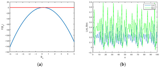
Figure 1.
Dynamics of the FDCV model (20) for ; (a) Equilibrium condition given by the nonlinear function ; (b) time series of and emerged from the initial condition .
To further verify the well-posedness and robustness of the proposed model (20), we conducted additional simulations by varying the parameter while keeping the remaining parameters fixed at , , , , , , , and , with . Three representative values of were considered, and the corresponding trajectories are displayed in Figure 2. As observed, despite variations in , all trajectories remain bounded and consistent, confirming that the model maintains well-posed behavior under small parameter perturbations.
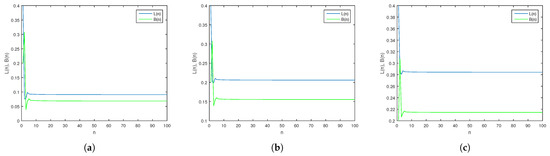
Figure 2.
Verification of well-posedness under variations of the parameter : (a) , (b) , (c) . All trajectories remain bounded and consistent.
4. Dynamics of the Fractional-Order Discrete System
In this section, we numerically investigate the dynamical behavior of the proposed fractional-order discrete computer virus (FDCV) model (20) under variations in key system parameters under commensurate and incommensurate orders. Our analysis is based on bifurcation diagrams, Maximum Lyapunov Exponents (), 0–1 test, Spectral Entropy (SE), and complexity, and aims to reveal the emergence of complex dynamical patterns, including chaos.
We investigate the chaotic behavior in the model (20) by exploiting the maximum Lyapunov exponent. It should be noted that it can be approximated using the Jacobian matrix algorithm [24].
such that
Then, we can get the Lyapunov exponents as:
where are the Jacobian matrix’s eigenvalues.
The fractional memory is inherently included in the Lyapunov exponent calculation via the Caputo-like delta operator. The summation in Equation (30) accounts for the contribution of past states, ensuring that the computed Lyapunov exponents reflect the full memory-dependent dynamics of the system.
4.1. Commensurate Case
We focus on how changes in the recruitment rate and the fractional order influence the long-term evolution of the system.
4.1.1. Dynamics of the FDCV Model with Variation in the Parameter
We first explore how the system’s dynamics are affected by the parameter . The L-nodes representing latent infected computers are connected to the internet and are recruited into the system at a constant rate . By simulating the model for different values of , while keeping all other parameters fixed at , and initial conditions , we observe a range of behaviors. The analysis is conducted across three different fractional orders: , , and .
As depicted in Figure 3, the bifurcation diagrams Figure 3a,c,e illustrate the long-term behavior of the state variable B as is varied for , respectively. Concurrently, Figure 3b,d,f present the corresponding Maximum Lyapunov Exponent () plot. For (Figure 3a,b), initially for small values of , the system exhibits chaotic behavior, indicating sensitive dependence on initial conditions. This chaotic behavior is strongly corroborated by the positive values of in Figure 3b. Interestingly, within the chaotic region, there are several periodic windows around , where the system temporarily goes to periodic behavior, identified by narrower bands in the bifurcation diagram and a dip in to negative values. Beyond these windows, chaos re-emerges and persists for larger values, with remaining predominantly positive, signifying robust chaotic dynamics. A similar progression is observed for (Figure 3c,d) and (Figure 3e,f). While the specific onset points and widths of chaotic and periodic windows may vary slightly with , the overall qualitative behavior remains consistent: an initial periodic phase, followed by period-doubling leading to chaos, punctuated by periodic windows, and finally sustained chaos as increases. The positive values consistently confirm the presence of chaos in the regions of the bifurcation diagrams, while negative values align with the periodic windows. Notably, the overall range of chaotic behavior appears to broaden as approaches 1, indicating that higher fractional orders might promote more sustained chaotic dynamics under these parameter settings. In some simulations, small negative values of occur. These should be regarded as numerical artifacts of the discretization rather than physically meaningful outcomes. It is worth noting that the coefficients of the fractional sum are positive for . Hence, when all parameters and initial conditions are nonnegative, the analytical solution preserves nonnegativity in the absence of numerical errors. The small negative oscillations observed in are therefore attributed to round-off effects rather than to a violation of the model’s invariance properties. Developing positivity-preserving schemes for fractional discrete systems will be an important subject of future work.
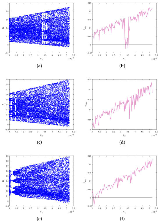
Figure 3.
Bifurcation diagrams and corresponding plots of the FDCV model (20) as a function of for different fractional orders: (a,b) , (c,d) , and (e,f) .
Based on the phase portraits and 0–1 test plots in Figure 4, the FDCV model (20) at a fractional order of undergoes a transition from chaotic to periodic behavior and then back to chaos as the parameter is varied. At , the system is in a chaotic state, as evidenced by the complex chaotic attractor in the phase portrait (Figure 4a) and the unbounded random walk observed in the 0–1 test in Figure 4d. As increases to , the system becomes regular, with its trajectory converging to a stable limit cycle in Figure 4b, and the 0–1 test plot showing a bounded orbit in Figure 4e. For a higher value of , the system returns to a chaotic state, confirmed by the appearance of a new chaotic attractor in Figure 4c and the renewed unbounded random walk in the 0–1 test in Figure 4f.
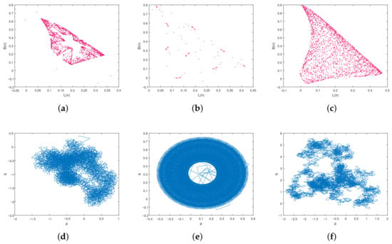
Figure 4.
Phase portraits and 0–1 test of the FDCV model (20) for with (a,d) , (b,e) , and (c,f) .
Figure 5a presents the Spectral Entropy (SE) as a function of . As increases, the SE generally shows an increasing trend, particularly in regions where the bifurcation diagrams indicate chaos and MLEs are positive. The dips in the SE curve correlate well with the periodic windows observed in the bifurcation diagrams, where the system temporarily becomes more predictable. Similarly, Figure 5b illustrates the complexity. The trend in the complexity plot mirrors that of the SE; it generally increases with , indicating growing complexity, and exhibits drops corresponding to the periodic windows where the system’s behavior becomes more regular.
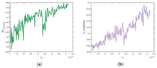
Figure 5.
SE and complexity of the FDCV model (20) for . (a) Spectral Entropy (SE), (b) complexity.
The combined evidence from the bifurcation diagrams, plots, phase portraits, 0–1 test, Spectral Entropy, and complexity consistently demonstrates that the FDCV model (20) exhibits a rich array of dynamical behaviors, transitioning from periodicity to chaos through period-doubling bifurcations as the rate increases. The presence of periodic windows within the chaotic regime further adds to the system’s intricate dynamics, which are robustly confirmed across different fractional orders. The quantitative measures (, SE, ) and qualitative test (0–1 test) effectively corroborate the visual insights gained from the bifurcation diagrams.
4.1.2. Dynamics of the FDCV Model with Variation in the Fractional Order
Next, we study the influence of the fractional order , which captures the memory effect inherent in the system. We assess how the memory strength affects the system’s evolution. To illustrate this effect, we fix all other parameters at and , and consider different values of while varying in the interval . The bifurcation diagrams and maximal Lyapunov exponent () plots reveal how the system’s behavior changes with the fractional order. For , the system exhibits both chaotic and ordered behaviors as is varied. The bifurcation diagram in Figure 6a shows that the system starts in a chaotic state for and undergoes several transitions, with a distinct periodic window emerging around . The corresponding plot in Figure 6b confirms this, with positive values in the chaotic regions and a clear drop to negative values in the periodic window, indicating a stable, ordered state. When the parameter is increased to , the system’s dynamics become robustly chaotic. As seen in the bifurcation diagram in Figure 6c, the system remains chaotic across the entire range of from to 1, with no clear periodic windows. This is supported by the plot in Figure 6d, which shows consistently positive values throughout the interval, confirming the persistent chaotic nature of the dynamics. For this value of , the system also appears to be entirely chaotic. The bifurcation diagram in Figure 6e shows a dense distribution of points with no visible periodic windows. The corresponding plot in Figure 6f is consistently positive, reinforcing the conclusion that the system remains chaotic across the entire range of from to 1. The analysis of Figure 6 demonstrates that the fractional order can act as a bifurcation parameter for the FDCV model (20), inducing transitions between chaos and order, particularly for smaller values of . However, as increases, its influence on the system’s dynamics appears to dominate, leading to a consistently chaotic state that is robust against variations in the fractional order.
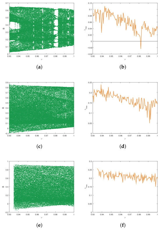
Figure 6.
Bifurcationand of the FDCV model (20) with (a,b) , (c,d) , and (e,f) .
To further characterize these behaviors, Figure 7 displays phase portraits and the 0–1 test for chaos for at representative fractional orders , , and . For and , the phase portraits reveal irregular chaotic attractors and the 0–1 test trajectories spread diffusively, indicating chaos. In contrast, for , the trajectory settles on a regular closed curve and the 0–1 test shows bounded motion, confirming periodic dynamics.
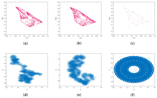
Figure 7.
Phase portraits and 0–1 test of the FDCV model (20) for with (a,d) , (b,e) , and (c,f) .
Figure 8 reports the spectral entropy (SE) and complexity measures for as functions of . Both indicators capture the complexity variation: higher values correspond to more irregular, chaotic dynamics, while lower values indicate more ordered regimes. These measures further validate the transitions observed in the bifurcation and Lyapunov exponent analysis.
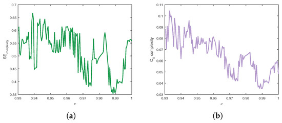
Figure 8.
SE and complexity of the FDCV model (20) for . (a) Spectral Entropy (SE), (b) complexity.
Overall, the results demonstrate that the fractional order plays a critical role in determining the qualitative dynamics of the FDCV model (20). Adjusting can effectively control the onset of chaos and complexity in computer virus propagation, offering potential for targeted mitigation strategies.
4.2. Incommensurate Case
Fractional-order systems with incommensurate orders form a generalized class of dynamical systems in which the fractional orders associated with each state variable are distinct and not rational multiples of one another. This configuration allows each state to exhibit different memory effects, providing a more flexible and realistic representation of the underlying processes. In this subsection, we investigate how incommensurate fractional orders influence the dynamic behavior of the FDCV model.
In the incommensurate case, each state is evaluated at a shifted time according to its fractional order.
4.2.1. Dynamics of the FDCV Model with Variation in
To explore the system’s behavior in the incommensurate setting (31), we begin by varying the fractional order , while keeping , and all other parameters fixed at . This approach enables us to isolate and analyze the specific impact of on the system’s stability, periodicity, and potential transition to chaotic dynamics. Figure 9a shows the bifurcation diagram, which indicates pronounced chaotic dynamics, with no discernible periodic windows and sustained irregularity. Figure 9b displays the corresponding largest Lyapunov exponent as a function of , which remains strictly positive for all tested values. This persistent positivity confirms the system’s sensitive dependence on initial conditions and the continuous presence of chaos throughout the examined interval.
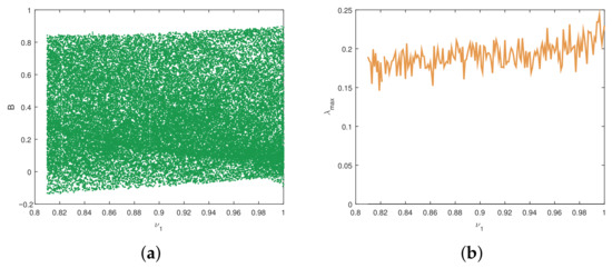
Figure 9.
Bifurcation and of the incommensurate FDCV model (31) versus for . (a) Bifurcation diagram, (b) .
For , the incommensurate FDCV model (31) exhibits clear signatures of strong chaotic behavior. The phase portraits in Figure 10a,b reveal complex, irregular attractors that densely occupy portions of the phase space, indicating the absence of periodic orbits. The results of the 0–1 test for chaos, shown in Figure 10c,d, display unbounded, diffusive trajectories in the -plane resembling a random walk, thereby providing compelling evidence of chaos. Collectively, these observations confirm that the model sustains robust chaotic dynamics for the specified fractional orders. The obtained trajectories remain bounded for all tested initial conditions and fractional orders, confirming that the system is numerically well-posed even when certain variables are unmeasured.
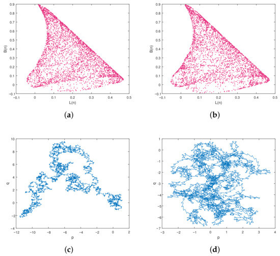
Figure 10.
Phase portraits and 0–1 test of the incommensurate FDCV model (31) for . (a,b) Phase portraits, (c,d) 0–1 test.
As varies with , the complexity measures reveal notable trends in the system’s dynamics. In Figure 11a, the Spectral Entropy (SE) remains relatively high (approximately –) throughout the range, with a slight upward tendency, indicating that unpredictability and irregularity intensify as increases. Figure 11b shows the complexity, which, despite some fluctuations, follows an overall increasing trajectory, suggesting that the richness and structural intricacy of the system’s behavior grow with larger fractional orders.
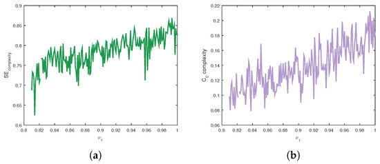
Figure 11.
SE and complexity of the incommensurate FDCV model (31) for . (a) Spectral Entropy (SE), (b) complexity.
4.2.2. Dynamics of the FDCV Model with Variation in
To further investigate the influence of the fractional-order parameter on the incommensurate FDCV model (31), we fix and vary . The bifurcation diagram in Figure 12a reveals that the system exhibits dense chaotic oscillations throughout the considered range, while the largest Lyapunov exponent in Figure 12b remains strictly positive, confirming the persistence of chaos. This indicates that fractional-order variation has a significant impact on the system’s chaotic dynamics. In the simulations, the Caputo-like delta operator was implemented using the full history without memory truncation. This ensures that the observed chaotic dynamics are intrinsic to the proposed FDCV model and not artifacts of the approximation.
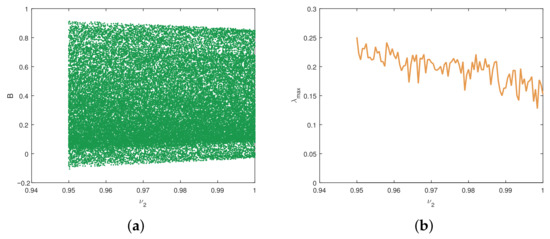
Figure 12.
Bifurcation and of the incommensurate FDCV model (31) versus for . (a) Bifurcation diagram, (b) .
Figure 13 illustrates phase portraits (a, b) and the 0–1 chaos test (c, d) of the incommensurate FDCV model (31) for two representative values of with . The phase portraits reveal irregular and non-periodic attractors, with in Figure 13a producing a denser structure compared to in Figure 13b, reflecting stronger chaotic mixing in the fractional-order case. The 0–1 test outputs (c, d) further validate chaotic dynamics: the trajectories in the (p,q)-plane spread out randomly for both values, with no bounded repetitive pattern. This provides numerical confirmation that the FDCV system (31) maintains chaotic behavior in both cases, though the structure is visibly richer at fractional orders.
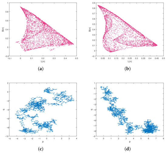
Figure 13.
Phase portraits and 0–1 test of the incommensurate FDCV model (31) for . (a,b) Phase portraits, (c,d) 0–1 test.
The complexity analysis presented in Figure 14 compares two complexity measures, Spectral Entropy (SE) and complexity for the incommensurate FDCV model (31) as varies within [0.94,1] while fixing . The SE values remain relatively high across the interval, showing a slight downward trend as increases, which suggests a gradual reduction in irregularity. Similarly, the complexity measure fluctuates irregularly but also decreases near . Together, these results indicate that the system retains significant complexity and unpredictability across the fractional range, with a tendency toward reduced complexity in . These results highlight the significant role of in shaping the chaotic and complex dynamics of the incommensurate FDCV model (31). In particular, fractional-order variations enhance the irregularity and richness of the attractors.
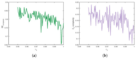
Figure 14.
SE and complexity of the incommensurate FDCV model (31) for . (a) Spectral Entropy (SE), (b) complexity.
5. Conclusions and Future Directions
In this paper, we developed and analyzed a fractional discrete-time computer virus (FDCV) model obtained by reformulating a three-dimensional continuous integer-order system into a two-dimensional discrete fractional framework. The model’s dynamical behaviors were investigated in both commensurate and incommensurate cases. Using bifurcation diagrams, the maximum Lyapunov exponent, phase portraits, the 0–1 test for chaos, and complexity indicators such as spectral entropy (SE) and complexity, we demonstrated that the proposed FDCV model exhibits rich chaotic dynamics and high complexity across wide parameter ranges. The results confirm that fractional-order discrete modeling provides deeper insights into the nonlinear and memory-dependent nature of computer virus propagation compared to classical integer-order approaches.
The study highlights the crucial role of fractional orders in shaping the dynamics of virus spread and shows that both commensurate and incommensurate systems preserve strong chaotic and complex behaviors. These findings contribute to the growing body of work on fractional discrete dynamical systems and underscore their relevance for understanding and modeling cybersecurity threats in modern technologies.
Future research may be pursued along several directions. One promising avenue is the introduction of control strategies into the FDCV model to suppress chaos or stabilize desirable behaviors. Another is the extension of the discrete fractional framework to other epidemiological-type computer virus models, such as SIS, SIR, and SEIR, which may provide further insights into different propagation mechanisms. Additionally, investigating synchronization phenomena in fractional discrete systems could open new perspectives for secure communication technologies. Finally, exploring numerical optimization techniques for parameter estimation may help align the theoretical model more closely with real-world network technologies and data. In addition, integrating the FDCV model with realistic network topologies (e.g., scale-free, small-world, and IoT infrastructures) constitutes another promising direction that will further enhance its applicability to real malware propagation scenarios.
Author Contributions
Conceptualization, A.A. and G.G.; Methodology, I.Z.; Software, I.Z.; Validation, A.M.; Formal analysis, I.Z. and G.C.; Investigation, I.Z. and A.O.; Resources, A.A. and A.O.; Data curation, A.M. and A.O.; Writing—original draft, I.Z.; Writing—review and editing, I.Z.; Visualization, I.Z.; Supervision, A.O. and G.C.; Project administration, A.O. and G.G.; Funding acquisition, A.M. and G.C. and G.G. All authors have read and agreed to the published version of the manuscript.
Funding
This research received no external funding.
Institutional Review Board Statement
Not applicable, as this study did not involve human or animal subjects.
Informed Consent Statement
Not applicable, as this study did not involve human participants.
Data Availability Statement
The original contributions presented in this study are included in the article; further inquiries can be directed to the corresponding author.
Conflicts of Interest
The authors declare no conflicts of interest.
References
- Szor, P. The Art of Computer Virus Research and Defense; Addison-Wesley Education Publishers Inc.: New York, NY, USA, 2005. [Google Scholar]
- Cohen, F. Computer viruses: Theory and experiments. Comput. Secur. 1987, 6, 22–35. [Google Scholar] [CrossRef]
- Piqueira, J.R.C.; Araujo, V.O. A modified epidemiological model for computer viruses. Appl. Math. Comput. 2009, 213, 355–360. [Google Scholar] [CrossRef]
- Yang, X.; Yang, L.X. Towards the epidemiological modeling of computer viruses. Discret. Dyn. Nat. Soc. 2012, 2012, 259671. [Google Scholar] [CrossRef]
- Yang, L.X.; Yang, X.; Zhu, Q.; Wen, L. A computer virus model with graded cure rates. Nonlinear Anal. Real World Appl. 2013, 14, 414–422. [Google Scholar] [CrossRef]
- Yuan, H.; Chen, G. Network virus-epidemic model with the point-to-group information propagation. Appl. Math. Comput. 2008, 206, 357–367. [Google Scholar] [CrossRef]
- Wu, G.C.; Baleanu, D. Discrete fractional logistic map and its chaos. Nonlinear Dyn. 2014, 75, 283–287. [Google Scholar] [CrossRef]
- Edelman, M.; Macau, E.E.; Sanjuan, M.A. Chaotic, Fractional and Complex Dynamics: New Insights and Perspectives; Springer: Berlin/Heidelberg, Germany, 2018. [Google Scholar]
- Zeng, J.; Chen, X.; Wei, L.; Li, D. Bifurcation analysis of a fractional-order eco-epidemiological system with two delays. Nonlinear Dyn. 2024, 112, 22505–22527. [Google Scholar] [CrossRef]
- El-Shahed, M.; Moustafa, M. Dynamics of a fractional-order eco-epidemiological model with two disease strains in a predator population incorporating harvesting. Axioms 2025, 14, 53. [Google Scholar] [CrossRef]
- Karaoğlu, E. On the Stability Analysis of a Fractional-Order Epidemic Model Including General Forms of Nonlinear Incidence and Treatment Functions. Commun. Fac. Sci. Univ. Ankara Ser. A1 Math. Stat. 2024, 73, 285–305. [Google Scholar] [CrossRef]
- Narwal, Y.; Rathee, S. Fractional order mathematical modeling of lumpy skin disease. Commun. Fac. Sci. Univ. Ankara Ser. A1 Math. Stat. 2024, 73, 192–210. [Google Scholar] [CrossRef]
- Kahouli, O.; Zouak, I.; Abu Hammad, M.; Ouannas, A.; Ayari, M. On an incommensurate chaotic fractional discrete model of a computer virus: Stabilization and synchronization. AIMS Math. 2025, 10, 19940–19957. [Google Scholar] [CrossRef]
- Abu Hammad, M.; Zouak, I.; Ouannas, A.; Grassi, G. Fractional Discrete Computer Virus System: Chaos and Complexity Algorithms. Algorithms 2025, 18, 444. [Google Scholar] [CrossRef]
- Kahouli, O.; Zouak, I.; Ouannas, A.; Abidi, I.; Bahou, Y.; Elgharbi, S.; Chaabane, M. Control and synchronization of chaos in some fractional computer virus models. Asian J. Control 2025, 27, 1–9. [Google Scholar]
- Kahouli, O.; Zouak, I.; Hammad, M.A.; Ouannas, A. Chaos, control, and synchronization in discrete-time computer virus system with fractional orders. AIMS Math. 2025, 10, 13594–13621. [Google Scholar]
- Abdeljawad, T. On Riemann and Caputo fractional differences. Comput. Math. Appl. 2011, 62, 1602–1611. [Google Scholar] [CrossRef]
- Atici, F.M.; Eloe, P. Discrete fractional calculus with the nabla operator. Electron. J. Qual. Theory Differ. Equ. 2009, 2009, 62. [Google Scholar] [CrossRef]
- Anastassiou, G.A. Principles of Delta Fractional Calculus on Time Scales and Inequalities. Math. Comput. Model. 2010, 52, 556–566. [Google Scholar] [CrossRef]
- Gottwald, G.A.; Melbourne, I. The 0–1 test for chaos: A review. Chaos Detect. Predict. 2016, 915, 221–247. [Google Scholar]
- He, S.; Sun, K.; Wang, H. Complexity Analysis and DSP Implementation of the Fractional-Order Lorenz Hyperchaotic System. Entropy 2015, 17, 8299–8311. [Google Scholar] [CrossRef]
- Shen, E.; Cai, Z.; Gu, F. Mathematical foundation of a new complexity measure. Appl. Math. Mech. 2005, 26, 1188–1196. [Google Scholar] [CrossRef]
- Yang, L.X.; Yang, X. A new epidemic model of computer viruses. Commun. Nonlinear Sci. Numer. Simul. 2014, 19, 1935–1944. [Google Scholar] [CrossRef]
- Wu, G.C.; Baleanu, D. Jacobian matrix algorithm for Lyapunov exponents of the discrete fractional maps. Commun. Nonlinear Sci. Numer. Simul. 2015, 22, 95–100. [Google Scholar] [CrossRef]


Disclaimer/Publisher’s Note: The statements, opinions and data contained in all publications are solely those of the individual author(s) and contributor(s) and not of MDPI and/or the editor(s). MDPI and/or the editor(s) disclaim responsibility for any injury to people or property resulting from any ideas, methods, instructions or products referred to in the content. |
© 2025 by the authors. Licensee MDPI, Basel, Switzerland. This article is an open access article distributed under the terms and conditions of the Creative Commons Attribution (CC BY) license (https://creativecommons.org/licenses/by/4.0/).