Aircraft Propeller Design Technology Based on CST Parameterization, Deep Learning Models, and Genetic Algorithm

Abstract

This article presents aircraft propeller optimal design technology; including an algorithm and OpenVINT 5 code. To achieve greater geometric flexibility, the proposed technique implements Class-Shape Transformation (CST) parameterization combined with Bézier curves, replacing the previous fully Bézier-based system. Performance improvements in the optimization process are accomplished through deep learning models and a genetic algorithm, which substitute XFOIL and Differential Evolution-based approaches, respectively. The scientific novelty of the article lies in the application of a neural network to predict the aerodynamic characteristics of profiles in the form of contour diagrams, rather than scalar values, which execute the neural network repeatedly per ISM algorithm iteration and speed up the design time of propeller blades by 32 times as much. A propeller for an aircraft-type UAV was designed using the proposed methodology and OpenVINT 5. A comparison was made with the results to solve a similar problem using numerical mathematical models and experimental studies in a wind tunnel.

1. Introduction

The propeller is an integral design element of an aircraft. Propeller shape optimization has become one of the most relevant problems due to the growth of unmanned aerial vehicle production [1,2]. The shape of the propeller affects the efficiency of the entire flight system and requires consideration of many factors and limitations [3,4]. Most early works mainly describe the influence of propeller shape on aerodynamic characteristics under design constraints [5]. This design methodology is based on the well-known work of Betz [6], who defined the condition for maximum propeller efficiency. As numerical design methods have been developed [7], software packages that allow for the implementation of propeller shape and characteristics have been developed. Many more sophisticated aerodynamic models have emerged, including the blade element method (BEM), blade element momentum theory (BEMT), vortex lattice method (VLM), computational fluid dynamics (CFD), and isolated section method (ISM) [1,8,9]. The propeller shape optimization problem is a multidisciplinary design problem (MDO), and the most commonly used methods for solving this problem are gradient and gradient-free methods [10,11]. In addition, the most widely used evolutionary algorithms are the standard genetic algorithm (GA) and particle swarm optimization (PSO) [12,13]. In recent years, machine learning methods have been increasingly used to solve this problem [14]. Neural networks are well suited to solving multidimensional, multiscale, and nonlinear problems [15].

The authors of this article have already investigated the issue of screw shape optimization [16]. This algorithm was developed to address the need for accelerating the optimal design process of propellers used in aviation engines. OpenVINT 4 integrates the following methodologies: Bézier curves for modeling propeller blade geometry [17,18]; the Isolated Sections Method (ISM) for computing the thrust generated by the propeller and its required power [19]; XFOIL for calculating the aerodynamic characteristics of blade cross-sectional profiles [20]; and Success-History-based Adaptive Differential Evolution (SHADE) to perform optimization [21]. Based on the results presented in [16], OpenVINT 4 was shown to compute the aerodynamic characteristics of propellers that align closely with wind tunnel test data, with approximately 3.5% variation. Furthermore, it demonstrated the ability to generate propellers with superior aerodynamic performance compared to commercial counterparts. OpenVINT 4 can generate an optimal propeller design in approximately 3 h of computation time. While this duration is considered relatively acceptable for analyzing a single specific case, it becomes impractical when the algorithm is required to design propellers for multiple aircraft configurations, such as in aircraft-wide optimization processes. Among the future work of the authors is the development of an algorithm suitable for aircraft design, specifically during the conceptual design stages. This algorithm is also planned to provide propeller proposals based on the aircraft configuration. For this reason, the authors have identified the OpenVINT 4 algorithm as a suitable option; however, it is necessary to reduce its computational time to make it usable in conceptual design phases.

An analysis of the computational subprocesses within OpenVINT 4 revealed that the calculation of XFOIL-based aerodynamic coefficients for cross-sectional profiles is the most time-consuming step. The most viable solution to accelerate this process is to replace XFOIL with a neural network. Modern architectures specialized in predicting the aerodynamic characteristics of airfoils or aerodynamic bodies are now available, achieving predictions that are highly consistent with training data while requiring minimal inference times [22,23,24]. In OpenVINT 4, the SHADE algorithm was employed due to its rapid convergence in multimodal, high-dimensional problems and its compatibility with population size reduction methods, specifically the Continuous Adaptive Population Reduction (CARP) method [25]. However, SHADE has the drawback of potentially becoming trapped in local optima if the population diversity is lost [21]. This algorithm helped mitigate the high computational costs associated with XFOIL calculation of the aerodynamic coefficients of the cross-sectional profiles.

This paper describes a propeller design technology based on CST parameterization and deep learning models of aerodynamic contour diagrams. In addition to integrating neural networks into the new version of the algorithm (OpenVINT 5), the parameterization of propellers was enhanced, particularly for modeling the cross-sectional profiles of propeller blades (airfoils), using the CST (Class-Shape Transformation) method [26]. This method offers greater flexibility in modeling diverse airfoil geometries than Bézier curves [27,28]. The other geometric features of the blade are described using Bézier curves. In OpenVINT 5, XFOIL was replaced with a neural network, thereby eliminating computational bottlenecks in the objective function evaluation. Consequently, the optimization algorithm was switched to one with a lower risk of premature convergence and the ability to explore broader search space regions. We selected a genetic algorithm because its genetic operators inherently maintain population diversity [29]. Although genetic algorithms exhibit slower convergence than SHADE, the accelerated objective function computation offsets this limitation. Furthermore, genetic algorithms allow for integrating population size reduction strategies [30], enhancing scalability. In this initial release of the algorithm, its functionality is designed specifically for generating propellers operating in incompressible flow. Future releases will be expanded to include compressible flows.

The scientific novelty of the article lies in the application of a neural network to predict the aerodynamic characteristics of profiles in the form of contour diagrams, rather than scalar values, which execute the neural network repeatedly per ISM algorithm iteration and significantly speed up the design time of propeller blades. In addition, the use of modern flexible and stable CST profile parameterization and a genetic algorithm for finding optimal values allows efficient propeller shapes to be obtained.

The article is structured as follows: Section 2 details the methodologies comprising the OpenVINT 5 algorithm, including the architecture of the neural network used to predict aerodynamic coefficients; Section 3 outlines the neural network configuration and its performance compared to XFOIL, alongside a case study comparing the computational and aerodynamic performance of OpenVINT 4 and 5; and Section 4 gives the conclusions of this work.

2. Methods

The proposed propeller design technology implemented in the OpenVINT 5 algorithm solves the following optimization problem:

$$\begin{array}{cc}\hfill \min & \mathrm{W}(\xi ),\hfill \\ \hfill \text{such that}& T_{\mathit{obj}}-T_{\xi }<0,\hfill \\ & \xi ∊\Omega ,\hfill \end{array}$$

(1)

where W(ξ) is the power required by the propeller; T(ξ) is the thrust provided by the propeller; T_obj is the desired thrust; ξ is the design parameter vector; and Ω is the decision space. Unlike OpenVINT 4 [16], OpenVINT 5 implements new methods primarily focused on reducing computation time, increasing flexibility in propeller geometry, and maintaining global optimum identification during optimization.

Table 1. Methods implemented in OpenVINT versions 4 and 5.

	OpenVINT 4	OpenVINT 5
Propeller cross-section modeling	Bezier Curves	CST Method
Propeller blade body modeling	Bezier Curves	Bezier Curves
Propeller W and T calculation	ISM	ISM
Aerodynamic coefficient calculation for propeller cross-sections	XFOIL	Neural Network
Constrained-to-unconstrained optimization conversion	Penalty Function	Self-Adaptive Penalty Method (SAPM)
Optimization algorithm	SHADE	Genetic Algorithm

shows the methods implemented in OpenVINT versions 4 and 5.

As shown in Table 1, only blade body modeling and the method for calculating propeller W and T remain unchanged in the new version. The other methods and their implementations are described below.

2.1. CST Method

The CST parameterization method stands out for its balance of mathematical simplicity, design flexibility, and computational efficiency. The CST method combines a class function C(x) (defining global characteristics like thickness or camber) and a shape function S(x) (modifying local details). This enables adjustment of specific parameters (leading edge, maximum camber) without altering the rest of the geometry. Consequently, complex shapes can be created with few coefficients, facilitating exploration of optimal designs in optimization processes [26].

In the CST method, the upper and lower airfoil curves are represented as:

$$y(x)=C(x)S(x)+x\Delta y_{te},$$

(2)

where Δy_te denotes the trailing edge thickness of the airfoil (this term is omitted if the airfoil has a sharp trailing edge).

The class function for defining airfoil geometries is expressed as:

$$C(x)=\sqrt{x}(1-x),$$

(3)

while the shape function for generating arbitrary aerodynamic shapes is:

$$S(x)={\sum }_{r=0}^n\left(A_{r}BPn\right),$$

(4)

where BPn is the Bernstein polynomial given by:

$$BPn=\left({\displaystyle \genfrac{}{}{0pt}{}{n}{r}}\right)x^r{\left(1-x\right)}^{n-r},$$

(5)

The use of Bernstein polynomials guarantees smooth curves and surfaces, avoiding discontinuities that could cause flow separation.

Thus, the extended equations defining the airfoil’s upper and lower curves are:

$$y_u=\sqrt{x}(1-x){\sum }_{r=0}^n\left(A_{u,r}BPn\right),$$

(6)

$$y_l=\sqrt{x}(1-x){\sum }_{r=0}^n\left(A_{l,r}BPn\right),$$

(7)

where u is the subscript denoting the upper airfoil curve; l is the subscript denoting the lower airfoil curve; A_u,r and A_l,r are the coefficients of the Bernstein polynomial components; and x is a sequence of values between 0 and 1.

The thickness distribution and camber line of the airfoil are determined using:

$$y_t=2C(x){\sum }_{r=0}^n\left({\displaystyle \frac{A_{u,r}-A_{l.r}}{2}}\right)BPn,$$

(8)

$$y_c=C(x){\sum }_{r=0}^n\left({\displaystyle \frac{A_{u,r}+A_{l.r}}{2}}\right)BPn,$$

(9)

2.2. Neural Network

The objective of the neural network is to substantially reduce computation time for aerodynamic coefficients of propeller cross-sections while maintaining accuracy comparable to XFOIL.

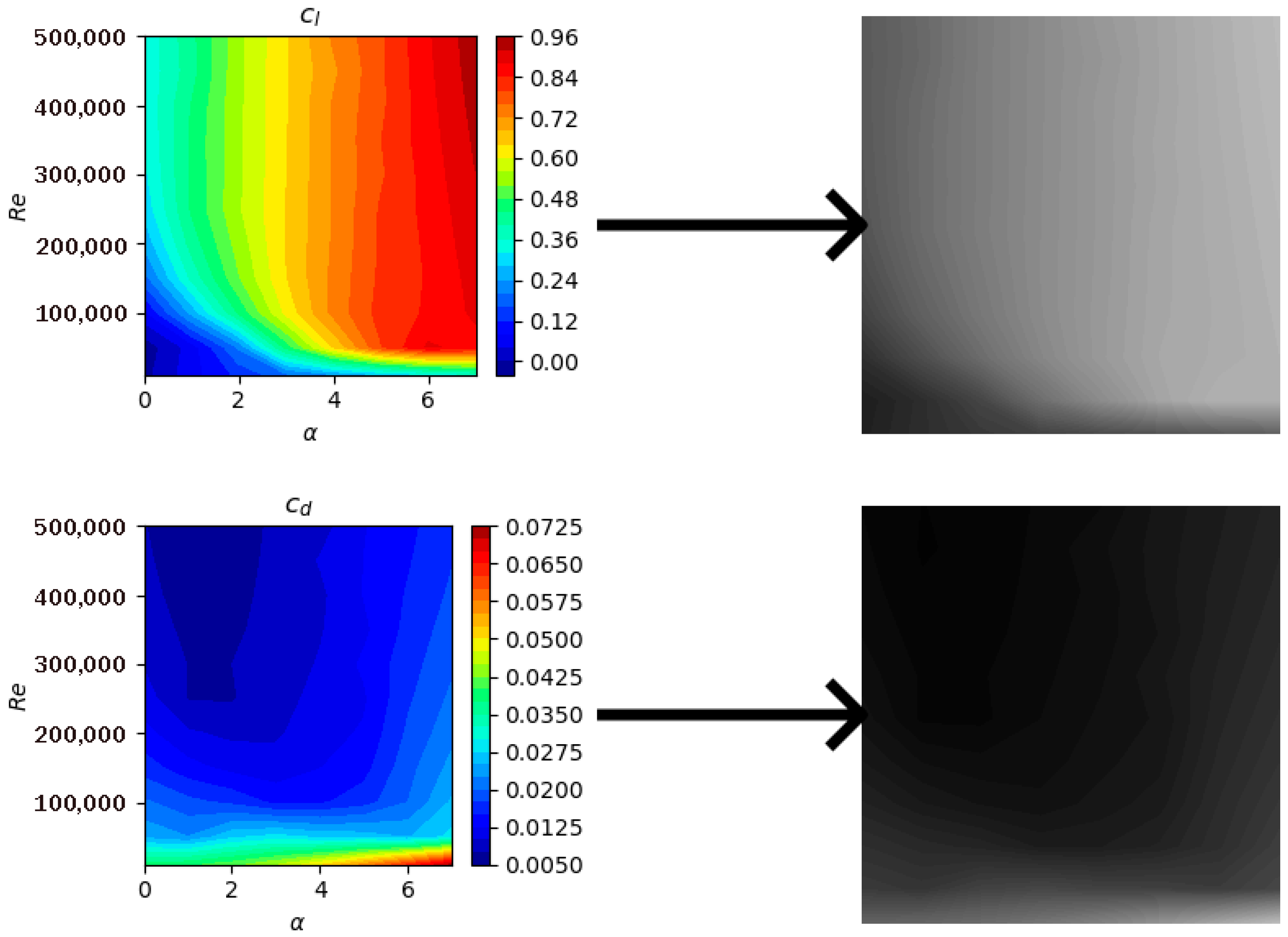
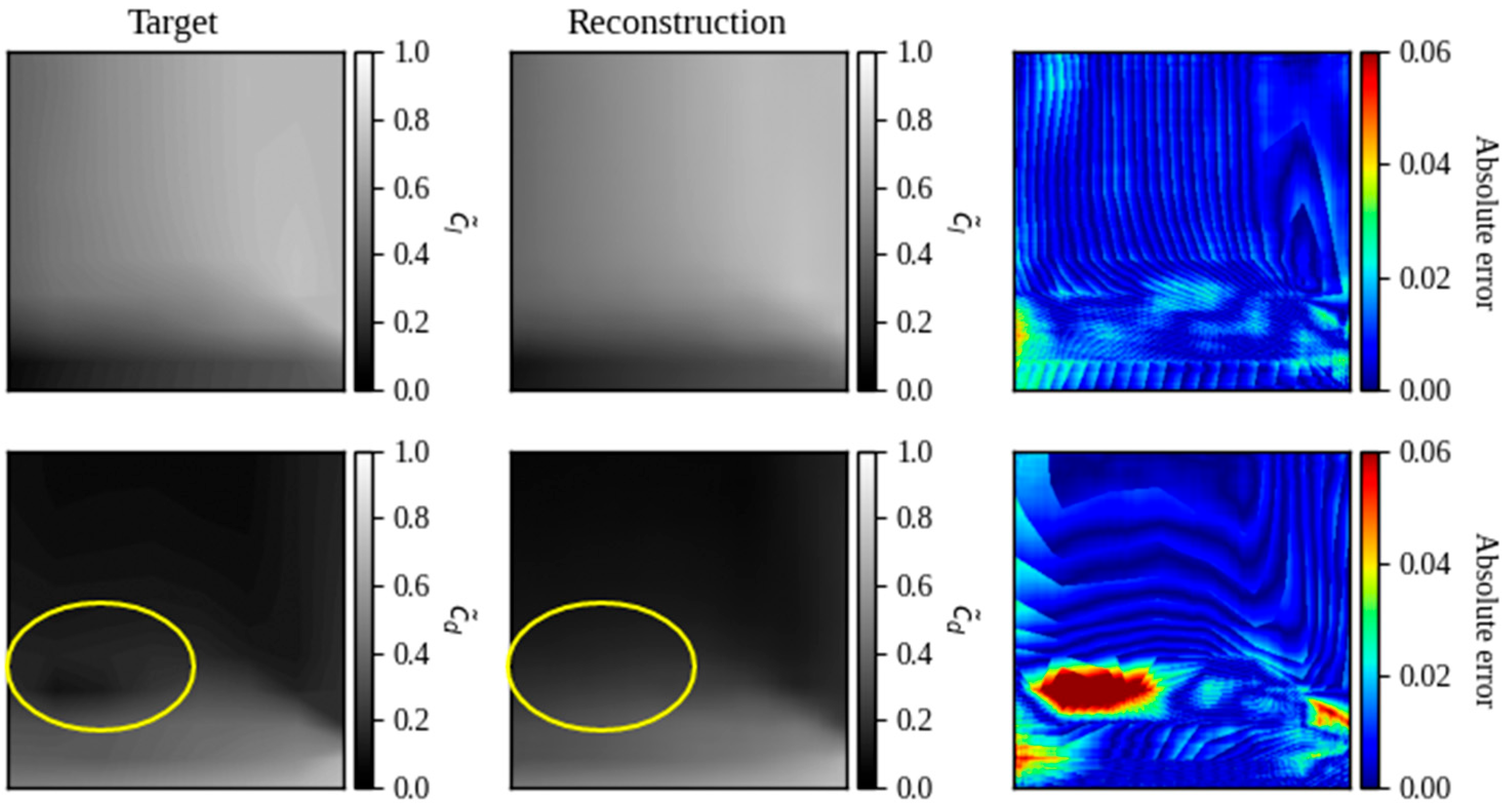
As in OpenVINT 4, this new version retains the modified ISM, which requires calculation of blade cross-section lift coefficients (c_l) and drag coefficients (c_d) as functions of: effective angle of attack (α) and local Reynolds number (Re) [16]. Therefore, it was considered that the neural network has as input vectors the parameters CST (which describe the geometry of a cross-section of the blade) and as output the contour plots of each aerodynamic coefficient (c_l and c_d) as a function of α and Re (see Figure 1).

One rationale for designing the neural network outputs as images (contour plots) rather than scalar values of c_l and c_d stems from compatibility requirements with the original ISM version (see Appendix A). This approach enables evaluation of designed propellers under diverse operating conditions (freestream velocities and revolutions per minute). As shown in Algorithm A1 (lines 9–22), the iterative process requires updating α at each step. Had scalar values been implemented as outputs, this would necessitate executing the neural network repeatedly per iteration to obtain aerodynamic coefficients. The contour plot implementation eliminates this requirement because:

• Each plot contains sufficient α-range data for multiple iterations;
• Predicted plots from a single inference cover multiple Re;
• Identical output plots serve different operating conditions without recomputation.

Furthermore, reference [22] demonstrates an additional advantage: the neural network implementation effectively eliminated inconsistencies (noise) in training data when using contour-based outputs.

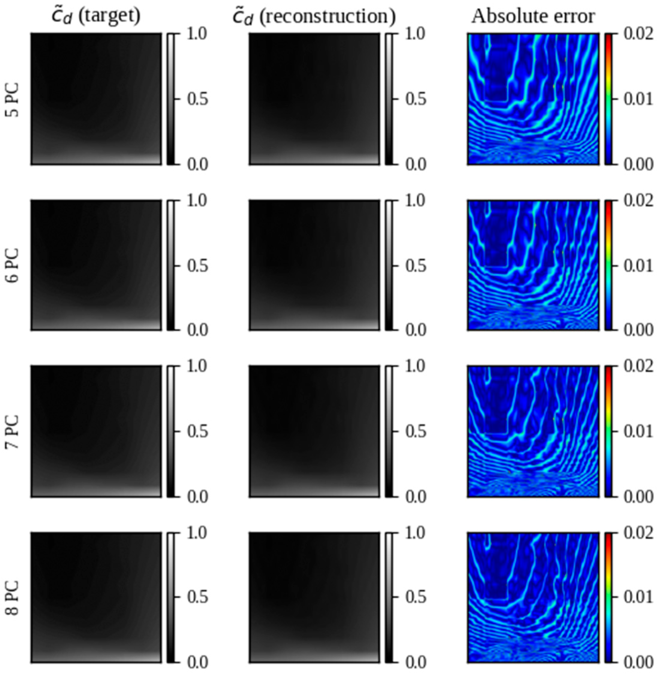
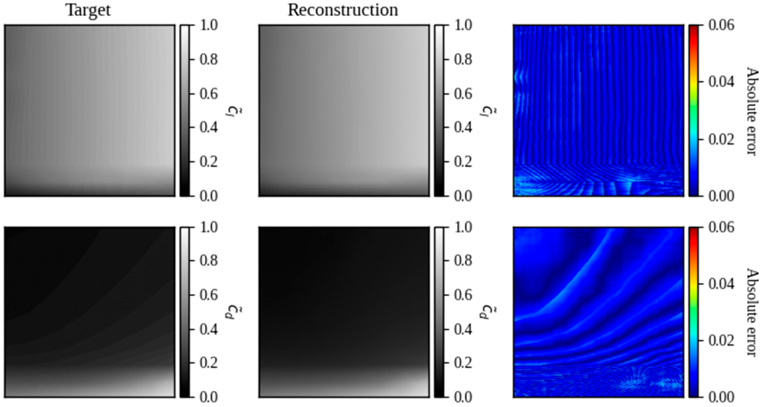
Having defined the input and output data types for the neural network, an architecture combining a multilayer perceptron (MLP) with a variational autoencoder (VAE) decoder was implemented. This hybrid structure has demonstrated efficacy in image prediction from input vectors in prior studies [22,31,32]. The hyperparameter determination process followed these steps:

• Use the Principal Components Analysis (PCA) [33,34] to obtain a first approximation of the representative features of the output images, which provides an initial estimate of the dimension of the latent vector (z) of a VAE;
• Use a VAE (see Figure 2) to extract the representative features of the output images through unsupervised learning;
• Develop an MLP to create a nonlinear mapping between the input parameters (parameters representing the geometry of the airfoils) and the features extracted by the VAE;
• Once the MLP is developed, it is connected to the decoder of the VAE, resulting in a neural network capable of predicting the contour plots of aerodynamic coefficients from a parameter vector representing the geometry of the airfoils (see Figure 3).

In [22], we provide further details on the architecture of the Encoder and Decoder of the VAE used (with the only difference being that in this work, only two layers (images) are considered for input and output, whereas ref. [22] uses three). Additionally, ref. [22] provides details on how to perform the hyperparameter selection for the MLP.

The database used for neural network training comprised 1500 airfoils with their respective aerodynamic coefficient contour plots (c_l and c_d). The input data correspond to the CST parameters, considering Bernstein polynomials of degree 5 for each curve, then the input vectors are formed by 12 parameters, 6 parameters for the upper curve (A_u,r) and 6 for the lower curve (A_l,r). To create the database, two subsets (training and testing) were considered. For training, 90% of the data was used, while 10% was allocated for testing (this data allocation ratio has yielded good results in training architectures composed of an MLP and a VAE [22,32]). The airfoils in each subset were generated by varying the CST parameters of the CLARK-Y airfoil between −40% and 40% (see

Table 2. CST parameters defining the CLARK-Y airfoil. Bernstein polynomials of degree 5 are considered.

Parameter	Value	Parameter	Value
Au,0	0.169295	Al,0	−0.154429
Au,1	0.337268	Al,1	−0.0150239
Au,2	0.0992323	Al,2	−0.121038
Au,3	0.389692	Al,3	0.0159202
Au,4	0.146156	Al,4	−0.0804828
Au,5	0.292191	Al,5	−0.0307818

and Figure 4). The CLARK-Y airfoil was selected due to its great use in the design of propellers [35]. Each subset was created using the Latin Hypercube Sampling technique; this technique ensures that the samples cover most of the design space in both subsets.

The contour plot data were obtained through simulations performed with XFOIL (the script used is shown in

Table 3. Example of the XFOIL script for obtaining aerodynamic coefficients of an airfoil [36].

Code	Operation
LOAD airfoil.dat	Load the coordinate file
MDES	Enter the MDES menu
FILT	Smooth any variations in the coordinate file
EXEC	Apply smoothing
	Return to the main menu
PANE	Set the number and location of airfoil points for analysis
OPER	Enter the OPER menu
ITER 50	Set the maximum number of iterations for convergence
RE 10000	Define the Reynolds number
VISC 10000	Enable viscous flow analysis with the specified Reynolds number
PACC	Initialize the output file to store aerodynamic coefficients
Coeffs.dat	Name of the output file
	Skip the dump file
ALFA 0	Calculate cl and cd at 0° angle of attack
ALFA 1	Calculate cl and cd at 1° angle of attack
…	…
ALFA 7	Calculate cl and cd at 7° angle of attack
PACC	Close the aerodynamic coefficients file
	Return to the main menu
QUIT	Exit XFOIL

). Prior to running XFOIL simulations, the coordinates (x, y) of each airfoil were extracted using the CST method and saved as dat text files. The values of α were set to 0°, 1°, 2°, 3°, 4°, 5°, 6°, and 7°, and Re were 10,000, 50,000, 100,000, 150,000, 200,000, 250,000, 300,000, 350,000, 400,000, 450,000, and 500,000.

To enhance training performance, both the input and output data were normalized [37,38]. For the normalization of input parameters, values were scaled to a 0–1 range using a MinMax scaler [33], with the transformation defined as:

$$A_{j,\mathrm{s}\mathrm{c}\mathrm{a}\mathrm{l}\mathrm{e}\mathrm{d}}={\displaystyle \frac{A_j-A_{j,\mathrm{m}\mathrm{i}\mathrm{n}}}{A_{j,\mathrm{m}\mathrm{a}\mathrm{x}}-A_{j,\mathrm{m}\mathrm{i}\mathrm{n}}}}.$$

(10)

where A_j,min and A_j,max represent the minimum and maximum values, respectively, of the parameter A_j.

For output data normalization, the aerodynamic coefficient values were first scaled to a 0–1 range using:

$$\tilde{c}={\displaystyle \frac{c-{0.9c}_{\mathrm{m}\mathrm{i}\mathrm{n}}}{{1.1c}_{\mathrm{m}\mathrm{a}\mathrm{x}}-{0.9c}_{\mathrm{m}\mathrm{i}\mathrm{n}}}}.$$

(11)

Subsequently, contour plots were generated using the contourf() function from Python 3.11. matplotlib library. The plots were created with 50 levels in a grayscale colormap (0 for black, 1 for white) [39]. The resulting images were saved in png format, excluding axes and labels, at a resolution of 256 × 256 pixels. Examples of the normalized plots are shown in Figure 5.

2.3. Genetic Algorithm and Self-Adaptative Penalty Method

For OpenVINT 5, a real-coded genetic algorithm was implemented. For this encoding scheme, the Simulated Binary Crossover (SBX) operator was employed [40,41], defined as:

$$c_{1,j}={\displaystyle \frac{1}{2}}\left((1-{\beta }_j)p_{1,j}+(1+{\beta }_j)p_{2,j}\right),$$

(12)

$$c_{2,j}={\displaystyle \frac{1}{2}}\left((1+{\beta }_j)p_{1,j}+(1-{\beta }_j)p_{2,j}\right),$$

(13)

where c₁ and c₂ are the offspring vectors derived from parent vectors p₁ and p₂; the subscript j denotes each parameter composing the vectors; and β_j is calculated as:

$${\beta }_j(u)=\left\{\begin{array}{ccc}{(2u)}^{{\displaystyle \frac{1}{{\eta }_c+1}}}& \mathrm{i}\mathrm{f}& u<0.5\\ {\displaystyle \frac{1}{{(2(1-u))}^{\frac{1}{{\eta }_c+1}}}}& \mathrm{e}\mathrm{l}\mathrm{s}\mathrm{e}& \end{array}\right.,$$

(14)

where u is a randomly sampled number from a uniform distribution between 0 and 1, and η_c is the crossover parameter.

The mutation operator employs a polynomial mutation strategy [41], defined as:

$$v_{i,j}=c_{i,j}+\left({\Omega }_j^u-{\Omega }_j^l\right){\delta }_j,$$

(15)

where v_i is the mutated vector derived from c_i; Ω_j^l and Ω_j^u are the minimum and maximum allowable values for parameter j, respectively; and δ_j is calculated as:

$${\delta }_j(u)=\left\{\begin{array}{ccc}{(2u)}^{{\displaystyle \frac{1}{{\eta }_m+1}}}& \mathrm{i}\mathrm{f}& u<0.5\\ {\displaystyle \frac{1}{1-{(2(1-u))}^{\frac{1}{{\eta }_m+1}}}}& \mathrm{e}\mathrm{l}\mathrm{s}\mathrm{e}& \end{array}\right.,$$

(16)

where η_m is the mutation parameter.

Since genetic algorithms do not directly solve constrained optimization problems, a penalty method is required to convert constrained problems into unconstrained formulations. For this new version, the SAPM was selected over penalty functions described in [42], eliminating the need for user-defined parameters (such as U^∗ specified in [42]). In SAPM, an adaptive penalty function combines with a distance function to determine objective vector values. The distance function computes distance measures for each dimension of the objective space. The final objective value for each individual is then obtained by summing its distance value and penalty value [43].

The distance value d_i(ξ) is defined as:

$$d_i(\xi )=\left\{\begin{array}{ccc}\psi (\xi )& \mathrm{i}\mathrm{f}& r_f=0\\ \sqrt{{\tilde{f}}_i{(\xi )}^2+\psi {(\xi )}^2}& \mathrm{e}\mathrm{l}\mathrm{s}\mathrm{e}& \end{array}\right.,$$

(17)

where r_f is the ratio of the number of feasible vectors in the current population to the population size; ${\tilde{f}}_i$(ξ) is the normalized objective function value for each vector, obtained via:

$${\tilde{f}}_i(\xi )={\displaystyle \frac{f_i(\xi )-f_{\mathrm{m}\mathrm{i}\mathrm{n}}^i}{f_{\mathrm{m}\mathrm{a}\mathrm{x}}^i-f_{\mathrm{m}\mathrm{i}\mathrm{n}}^i}},$$

(18)

here, fⁱ_min and fⁱ_max are the minimum and maximum values of the objective function across the current population. ψ(ξ) quantifies constraint violations and is calculated as:

$$\psi (\xi )={\displaystyle \frac{1}{J}}{\sum }_{j=1}^J{\displaystyle \frac{{\varphi }_j(\xi )}{{\varphi }_{\mathrm{m}\mathrm{a}\mathrm{x}}^j}},$$

(19)

$${\varphi }_j(\xi )=\left\{\begin{array}{cc}\mathrm{m}\mathrm{a}\mathrm{x}(0,g_j(\xi ))& j=1,...,q\\ \mathrm{m}\mathrm{a}\mathrm{x}(0,|h_j(\xi )|-\delta )& j=q+1,...,J\end{array}\right.,$$

(20)

where ϕ^j_max is the maximum value of the j-th constraint violation across the current population; and J is the total number of constraints (inequalities and equalities).

In addition to the distance measure, two penalty functions are incorporated into the fitness value of infeasible vectors. These penalties are formulated as:

$$\Psi (\xi )=(1-r_f){\chi }_i(\xi )+r_f{\rm Y}(\xi ),$$

(21)

$${\chi }_i(\xi )=\left\{\begin{array}{ccc}0& \mathrm{i}\mathrm{f}& r_f=0\\ \psi (\xi )& \mathrm{e}\mathrm{l}\mathrm{s}\mathrm{e}& \end{array}\right.,$$

(22)

$${{\rm Y}}_i(\xi )=\left\{\begin{array}{ccc}0& \mathrm{i}\mathrm{f}& {\xi }_i-\mathrm{v}\mathrm{i}\mathrm{a}\mathrm{b}\mathrm{l}\mathrm{e} \mathrm{v}\mathrm{e}\mathrm{c}\mathrm{t}\mathrm{o}\mathrm{r}\\ {\tilde{f}}_i(\xi )& \mathrm{e}\mathrm{l}\mathrm{s}\mathrm{e}& \end{array}\right.,$$

(23)

The modified final objective value of vector ξ is formulated as the sum of the distance measure and the penalty function in the i-th objective function dimension:

$${\tilde{F}}_i(\xi )=d_i(\xi )+{\Psi }_i(\xi ),$$

(24)

The genetic algorithm incorporates an exponential population reduction method [30], where the population size at each generation g is defined as:

$$N_g={\left(N_0+\gamma \right)e}^{-c·g},$$

(25)

$$c={\displaystyle \frac{1}{G}}\left(-ln\left({\displaystyle \frac{N_f-\gamma }{N_0+\gamma }}\right)\right),$$

(26)

where γ is a parameter controlling the decay curve shape (typically set to 5); N_f is the minimum population size (typically set to 20); N₀ is the initial population size; and G is the total number of generations.

The implemented genetic algorithm follows these steps:

• Initialization: The N₀ vectors of the first generation are randomly generated.
• Aerodynamic Evaluation: Compute T and W for each vector using the modified ISM.
• Fitness Assignment: Calculate the modified objective value $\tilde{F}$ for each vector using the self-adaptive penalty method.
• Population Size Update: Calculate the next generation’s population size N_g using exponential decay.
• Elitism: Transfer the top N_E vectors (elite individuals) directly to the next generation population.
• Crossover:
  • Use a tournament selection operator to select two parent vectors.
  • Generate two offspring vectors via the SBX operator.
  • Repeat until N_g − N_E offspring vectors are created.
• Mutation: Apply the polynomial mutation strategy to all N_g − N_E offspring vectors.
• Population Merge: Combine the mutated offspring vectors with the elite vectors to form the next generation.
• Termination: Repeat Steps 2–8 until the maximum number of generations is reached or another stopping criterion is satisfied.

2.4. Code Implimentation

2.4.1. Design Variables

The design variables utilized in the OpenVINT 5 optimization process comprise three propeller characteristics that vary with propeller radius: chord relative to propeller diameter (c/d), effective angle of attack of the cross-section (α), aerodynamic twist (Δ_us, Δ_ls). Following the approach in [16], smooth variation in these characteristics along the blade is achieved through two second-degree Bézier curves. These curves are defined as:

$$B_{\overline{r}}(t)={(1-t)}^2{\overline{r}}_0+2(1-t)t{\overline{r}}_1+t^2{\overline{r}}_2,$$

(27)

$$B_{\xi }(t)={(1-t)}^2{\xi }_0+2(1-t)t{\xi }_1+t^2{\xi }_2.$$

(28)

The control points for the root Bézier curve are defined as:

$$\left\{\begin{array}{c}{\overline{r}}_0^r=0.2\\ {\overline{r}}_1^r=0.5{\overline{r}}_{{\xi }_m}+0.5\\ {\overline{r}}_2^r={\overline{r}}_{{\xi }_m}\end{array}\right.\hspace{1em}\left\{\begin{array}{c}{\xi }_0^r={\xi }_r\\ {\xi }_1^r={\xi }_m\\ {\xi }_2^r={\xi }_m\end{array}\right..$$

(29)

For the tip Bézier curve, the control points are:

$$\left\{\begin{array}{c}{\overline{r}}_0^t={\overline{r}}_{{\xi }_m}\\ {\overline{r}}_1^t=0.5{\overline{r}}_{{\xi }_m}+0.485\\ {\overline{r}}_2^t=0.97\end{array}\right.\hspace{1em}\left\{\begin{array}{c}{\xi }_0^t={\xi }_m\\ {\xi }_1^t={\xi }_m\\ {\xi }_2^t={\xi }_t\end{array}\right..$$

(30)

In (29) and (30), ξ is replaced by c/d, α, Δ_us, and Δ_ls. Here, Δ_us and Δ_ls represent the combined variation in the CLARK-Y airfoil CST parameters for the upper and lower curves, respectively.

Additional parameters considered as design variables include: propeller diameter (d), number of blades (B), and revolutions per minute (n_m). Thus, given ${\overline{r}}_{{\Delta }_{us}m}={\overline{r}}_{{\Delta }_{ls}m}={\overline{r}}_{\Delta m}$, the complete set of design variables in OpenVINT 5 comprises: $\xi =\left[{(c/d)}_r,{(c/d)}_m,{(c/d)}_t,{\overline{r}}_{cm},{\alpha }_r,{\alpha }_m,{\alpha }_t,{\overline{r}}_{\alpha m},{\Delta }_{usr},{\Delta }_{usm},{\Delta }_{ust},{\Delta }_{lsr},{\Delta }_{lsm},{\Delta }_{lst},{\overline{r}}_{\Delta m},n_m, B, d\right]$.

2.4.2. Calculation of the Objective Function

To obtain the calculation of the thrust provided by the propeller and the power required by the propeller, OpenVINT 5 (like version 4) uses a modified version of the ISM (from Algorithm A1). The modification consists of taking the effective angles of attack of each cross-section of the blades as input parameters, and the installation angle becomes a calculated parameter (it becomes an output) (see Algorithm 1). This modification prevents the generation of α values that fall outside the neural network operational range (that is, values with which the neural network was not trained). Additionally, this modification places the calculation of the aerodynamic coefficients outside the loop responsible for computing the local velocities of the cross-sections.

Algorithm 1 shows the pseudocode for calculating W and T. In the algorithm, in addition to showing the steps of the ISM (including the modification mentioned above), the process for creating the Bezier curves of the input parameters such as c/d, α, Δ_us, and Δ_ls is shown. In Algorithm 1, the inputs are: P_g—design parameter vectors of the current population; physical properties of the freestream airflow (V_∞—velocity, ρ—density, and ν—kinematic viscosity); N—current population size; NS—number of blade cross-sectional sections; $\overline{r}$—relative position of each NS-section; namesDir—list of directory names for storing data of each simulated propeller in the current population. The outputs are: [T]—thrust generated by the propeller; [W]—power required by the propeller; [ϕ]—installation angle or geometric twist of each blade section; and [η_d], [η_s]—dynamic and static efficiency of the propeller. Variables enclosed in brackets (for example [T]) denote arrays storing values for all propellers in the current population.

Algorithm 1. Run objective function in OpenVINT 5
	$\mathbf{Inputs}\mathbf{:} P_g, V_{\infty }, \rho , \nu , N, \mathit{NS}, \overline{r}$, namesDir
	Outputs: [T], [W], [ϕ], [ηd], [ηs]
1	[n] = ∅, [d] = ∅;
2	[c/d] = ∅, [α] = ∅, [Re] = ∅, [A] = ∅;
3	for i = 1 to N do
4		Create directory namesDiri;
5		Get the values of c/d, α, Δus, and Δls of each section of the i-propeller with (27)–(30);
6		Get the CST parameters (A) of each section of the i-propeller;
7		c/d ⇾ [c/d], A ⇾ [A], α ⇾ [α];
8		From Pi,g extract nm and d;
9		d ⇾ [d], nm/60 ⇾ [n];
10		Calculate Re in each section of the blade;
11		Re ⇾ [Re];
12	Normalize [A];
13	[IC] = run_nn([A]);
14	[cl] = ∅, [cd] = ∅;
15	for k = 1 to N*NS do
16		cl, cd = read_coeffs([α]k, [Re]k, [IC]k);
17		cl ⇾ [cl], cd ⇾ [cd];
18	[W] = ∅, [T] = ∅, [ηd] = ∅, [ηs] = ∅;
19	[ϕ] = ∅
20	for i = 1 to N do
21		Extract the corresponding data from the i-helix of [c/d], [α], [d], [n], [cl] and [cd];
22		$0\to {\overline{u}}_1, 0\to \left({\int }_{\overline{r}}^1{\displaystyle \frac{{\overline{u}}_1^2}{\overline{r}}}d\overline{r}\right)$;
23		Get ω$\mathrm{and} \overline{v}$ with (A1) and (A2), respectively;
24		for t = 1 to 10 do
25			Iu = ∅;
26			for s = 1 to NS do
27			$\hspace{1em}\mathrm{Get} {\overline{v}}_{1_s}$ with (A3);
28			$\hspace{1em}\mathrm{Get} {\overline{U}}_{1_s}$ with (A4);
29			$\hspace{1em}\mathrm{Get} {\overline{V}}_{1_s}$ with (A5);
30			$\hspace{1em}\mathrm{Get} {\overline{W}}_{1_s}$ with (A6);
31			$\hspace{1em}\mathrm{Get} {\beta }_{1_s}$ with (A7);
32			$\hspace{1em}{\varphi }_s={\alpha }_s+{\beta }_{1_s}$;
33			$\hspace{1em}{K}_s=c_{l_s}/c_{d_s}$;
34			$\hspace{1em}\mathrm{Get} {\sigma }_s$ with (A8);
35			$\hspace{1em}\mathrm{Get} {\overline{\Gamma }}_{r_s}$ with (A9);
36			$\hspace{1em}\mathrm{Get} f_{r_s}$ with (A10);
37			$\hspace{1em}\mathrm{Update} {\overline{u}}_{1_s}$ with (A11);
38			$\hspace{1em}{\overline{u}}_{1_s}^2/{\overline{r}}_s\to I_{u_s}$;
39			for s = 1 to NS do
40			$\hspace{1em}\mathrm{Get} {\left({\int }_{\overline{r}}^1{\displaystyle \frac{{\overline{u}}_1^2}{\overline{r}}}d\overline{r}\right)}_s$$\mathrm{with} \mathrm{trapz}(I_u[s:\mathbf{end}], \overline{r}$[s:end]);
41		ϕ ⇾ [ϕ];
42		for s = 1 to NS do
43			$\mathrm{Get} {dc}_{t_s}$$\mathrm{and} {dm}_{k_s}$ with (A12) and (A13), respectively;
44		$c_t=\mathrm{t}\mathrm{r}\mathrm{a}\mathrm{p}\mathrm{z}(d{c}_t,\overline{r})$;
45		$m_k=\mathrm{t}\mathrm{r}\mathrm{a}\mathrm{p}\mathrm{z}(d{m}_k,\overline{r})$;
46		Get αp, βp and λp with (A16), (A17) and (A18), respectively;
47		Get T, W, ηd and ηs with (A14), (A15), (A19) and (A20), respectively;
48		T ⇾ [T], W ⇾ [W], ηd ⇾ [ηd], ηs ⇾ [ηs];
49		Save information in namesDiri;
50	return Outputs

2.4.3. Blade Geometry Construction

In OpenVINT 5, the blade geometry is generated through the following steps:

• Obtain the airfoil geometry for each section using the CST method;
• Calculate the position of the maximum thickness (x_t,max) of each airfoil section using (8);
• Scale the airfoils of each section according to their corresponding chord length;
• Define the blade twist axis, which intersects the chord line at the x_t,max point;
• Position and rotate the airfoil sections about the twist axis by ϕ degrees (the ϕ value for each section is determined using Algorithm 1).

Figure 6 shows a propeller constructed from the cross-sections generated by OpenVINT. OpenVINT 5 includes functionality to save the blade cross-section coordinates (x, y, z) as DAT text files, enabling seamless integration with SIMENS NX 8.5 software for propeller visualization.

2.4.4. OpenVINT 5 Algorithm

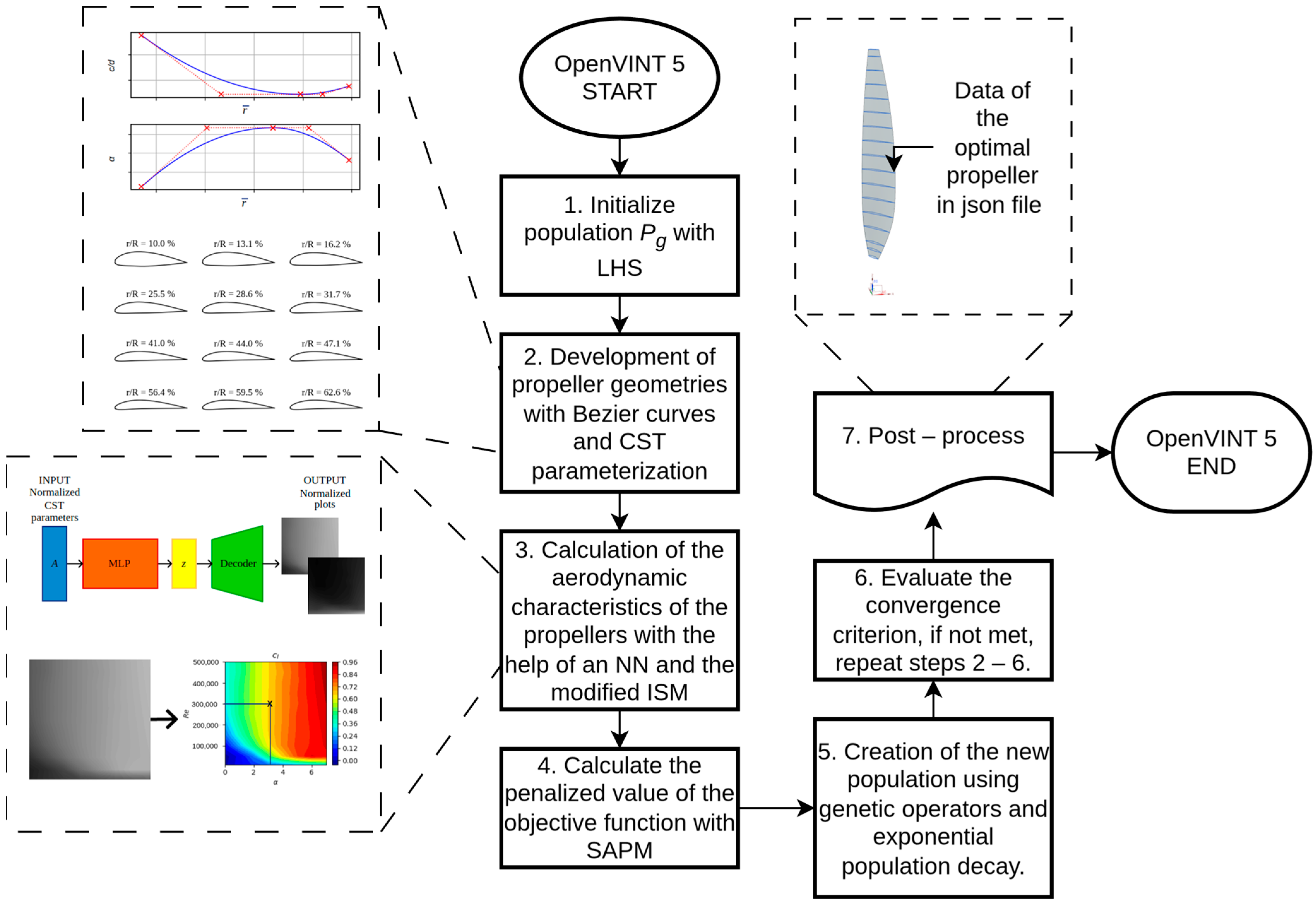
Algorithm 2 shows the pseudocode of OpenVINT 5, while Figure 7 shows how OpenVINT 5 operates schematically, highlighting the main routines.

Algorithm 2. OpenVINT 5 algorithm
	Inputs: Ω, V∞, ρ, ν, N, G, Tobj, name_case;
	Outputs: ξopt, Wopt, Topt, ηd,opt, ηs,opt;
1	Load the architecture and weights of the neural network;
2	Create folder name_case;
3	g = 1;
4	Create folder name_case/Generation_+str(g);
5	Initialize the population P1(ξ) with Latin_Hypercube_Sample(N, Ω);
6	for i = 1 to N0
7		Create folder name_case/Generation_+str(g)/blade_+str(i) (nameDiri);
8	Run Algorithm 1;
9	Calculate the modified objective value $\tilde{F}$ for each vector using SAPM;
10	for g = 2 to G;
11		Create folder name_case/G+str(g);
12		Calculate Ng with (25) and (26);
13		Apply elitism operator;
14		Apply crossover operator;
15		Apply mutation operator;
16		Population update Pg(ξ);
17		for i = 1 to Ng
18			Create folder name_case/Generation_+str(g)/blade_+str(i);
19		Run Algorithm A1;
20			Calculate the modified objective value $\tilde{F}$ for each vector using SAPM;
21	Extract ξopt from PG(ξ);
22	Create folder name_case/blade_opt;
23	Save information of optimal blade in name_case/blade_opt;
24	return Outputs;

In [44] the repository of the OpenVINT algorithm scripts is made available to the reader, in addition the scripts used for the training of the neural network are included.

3. Results and Discussion

3.1. Neural Network Training Results

For the determination of the neural network hyperparameters, PCA was first applied to one of the encoded images from the contour plots. Based on [22,32], it was proposed to analyze between 5 and 8 principal components (PC). Figure 8 and Figure 9 show the reconstructions performed using PCA for each of the normalized fields (${\tilde{c}}_l$ and ${\tilde{c}}_d$). The analyses yielded average image reconstruction errors of up to 2% for the case of 5 PCs. Therefore, it was considered to perform the VAE training with latent z vectors with dimensionality close to 5.

Three VAEs with latent vector dimensions of 5, 6, and 7 were trained to determine the optimal dimensionality of z. The VAEs was trained using the Adam optimizer, which was subjected to a learning rate schedule (specifically ExponentialDecay, with the following arguments: initial_learning_rate = 0.001, decay_steps = 2250, and decay_rate = 0.8). The batch size was set to 32 with a maximum of 300 epochs. EarlyStopping regularization tool from Keras was employed to halt training automatically when validation metrics ceased improving, thereby mitigating overfitting [45]. EarlyStopping callback was implemented with a patience value of 20. The loss function consisted of a combination of Binary Cross-Entropy and KL-Divergence. For evaluation, the Mean Absolute Error (MAE) metric was employed. Figure 10 and

Table 4. MAE values for image reconstruction using VAEs (testing phase).

Latent Dimension	MAE		MAE Global Average
	cl	cd
5	0.0077	0.0067	0.0072
6	0.0082	0.0067	0.0075
7	0.0080	0.0066	0.0073

present the testing phase results for the three latent vector dimensions.

The results indicated that all three latent vector dimensions achieved comparable reconstructions. However, the 5-dimensional latent vectors generally yielded the most accurate reconstructions.

Figure 11 illustrates an example of contour plot reconstructions using a 5-dimensional latent vector. As shown, the reconstruction errors are negligible. In some cases, the VAE even smoothed regions of the c_d contour plots. Figure 12 demonstrates a scenario where the c_d contour plot exhibited a small region with anomalously low c_d values caused by XFOIL convergence inconsistencies. The VAE effectively eliminated this noise.

To determine the optimal architecture for the MLP, the configurations listed in

Table 5. Tested MLP configurations.

Configuration	Layers and Neurons	Activation Function	MSE	R2avg
1	12-32-5	ReLU	0.0053	0.9084
2	12-32-32-5	ReLU	0.0031	0.9398
3	12-32-32-32-5	ReLU	0.0033	0.9347
4	12-32-32-5	Leaky ReLU	0.0043	0.9249
5	12-32-32-5	Tanh	0.0032	0.9363
6	12-64-32-5	Tanh	0.0037	0.9292
7	12-64-64-5	Tanh	0.0042	0.9246

were evaluated. The MLPs were trained using the ADAM optimizer (with a learning rate of 0.001), a batch size of 32, and 10% of the training data reserved for validation. The mean squared error (MSE) was employed as the loss function, and the coefficient of determination (R²) was utilized as the evaluation metric. EarlyStopping callback was implemented with a patience value of 20.

Configuration 5—featuring two hidden layers with 32 neurons each and hyperbolic tangent (Tanh) activation functions—achieved the best mapping between geometric parameters and latent vectors of the images. During testing, it yielded an MSE of 0.0032 and an average R² of 0.9363. Figure 13 details the R² analysis for each of the five latent vector z components.

The neural network responsible for predicting aerodynamic coefficient contour plots comprises: an MLP with a 12-dimensional input layer, two 32-neuron hidden layers, a 5-dimensional output layer connected to a decoder.

The MLP + Decoder ensemble generates output images (e.g., Figure 5), which undergo an inverse transformation using (11) to accurately extract c_l and c_d values. Figure 14 compares decoded contour plots with those generated using XFOIL.

To evaluate the neural network generalization capability, the R² metric was applied (see Figure 15).

The R² results of the proposed neural network are similar to those provided by other neural networks dedicated to predicting airfoil aerodynamic coefficients (R²∼0.99).

Table 6. Performance analysis of the prediction of the aerodynamic coefficients of different neural networks.

Neural Network	R2		Database Size	Main Features
	cl	cd
OpenVINT 5 NN (MLP + Decoder)	0.9881	0.9820	1500	Supports airfoils parameterized with the CST method (based on the CLARK-Y profile); For each input vector (airfoil parameters), two images are generated, each containing information about one aerodynamic coefficient (cl and cd) as a function of different α and Re. Limited to incompressible flow.
AZTLI-NN (MLP + Decoder) [22]	0.9933	0.9764	1000	Supports airfoils parameterized with the CST method; For each input vector (airfoil parameters), three images are generated, each containing information about one aerodynamic coefficient (cl, cd and cl1.5/cd) as a function of α. This is limited to a case of flow (Re = 1.5 × 106 and M = 0.15) (incompressible flow).
MLP [23]	0.9997	0.9092	1680	Supports 4-digit and 5-digit NACA airfoils; For each input vector (airfoil parameters, α, Re and M), a vector composed of three aerodynamic coefficients (cl, cd and cm) is generated. Although Re and M are considered as inputs, the ranges are limited from 1 × 105 to 5 × 106 for Re, and from 0.1 to 0.3 for M (limited to incompressible flow).
Radial Basis Function (RBF) [12]	0.9731 *	0.9731 *	208	Supports airfoils parameterized with the PARSEC method; For each input vector (airfoil parameters), a vector composed of five aerodynamic coefficients (cl, cd,w, cd,f, cd, cm, mcl/cd) is generated. Only one flow case was considered (Re = 2.3 × 107, M = 0.705) and one α value (2.53°).
General Regression Neural Network (GRNN) [12]	0.9807 *	0.9807 *	208	Supports airfoils parameterized with the PARSEC method; For each input vector (airfoil parameters), a vector composed of five aerodynamic coefficients (cl, cd,w, cd,f, cd, cm, mcl/cd) is generated. Only one flow case was considered (Re = 2.3 × 107, M = 0.705) and one α value (2.53°).

* The author did not provide the R² value for each individual aerodynamic coefficient, but rather provided an averaged R² value across the five aerodynamic coefficients.

shows a comparison with four other neural networks having different architectures. Within this comparison, the neural network for OpenVINT 5 stands out by being the only one capable of uniquely predicting aerodynamic coefficients at multiple angles of attack and Reynolds numbers in a single inference—a novel contribution at the time of writing this work.

The neural network predicts contour plots for 150 distinct airfoils in approximately 1.25 s. In contrast, XFOIL requires roughly 1 min to generate data for a single airfoil. Tests were conducted on a system with the following specifications:

• Processor: AMD Ryzen™ 7 5700G with Radeon™ Graphics × 16;
• RAM: 32 GB
• GPU: NVIDIA GeForce RTX 3060, 12 GB
• Operating System: Ubuntu 24.04.2 LTS

3.2. Performance Analysis of OpenVINT 5

To compare the performance between the two versions of OpenVINT, the following case study was considered:

“Design an optimal propeller for a fixed-wing aircraft engine, with a freestream air velocity (V_∞) of 33 m/s and a minimum required thrust (T_obj) of 28 N. The air properties are: ρ = 1.225 kg/m³; ν = 0.000014607 m²/s.”

In the optimization processes it was considered to calculate 4000 times the objective function. For Version 4, the initial population size was set to 100 individuals, a γ factor of 50, and an initial U^∗ value of 1500 W. For Version 5, a initial population size of 100 individuals was used, with η_c and η_m set to 20, and N_E equal to 2. The ranges of the design variables implemented in each algorithm are shown in

Table 7. The ranges of the design variables.

OpenVINT 4		OpenVINT 5
Variable	Range	Variable	Range
(c/d)r	[0.03, 0.05]	(c/d)r	[0.03, 0.05]
(c/d)m	[0.06, 0.12]	(c/d)m	[0.06, 0.12]
(c/d)t	[0.01, 0.02]	(c/d)t	[0.01, 0.02]
${\overline{r}}_{cm}$	[0.35, 0.60]	${\overline{r}}_{cm}$	[0.35, 0.60]
αr	[0, 7]°	αr	[0, 7]°
αm	[0, 7]°	αm	[0, 7]°
αt	[0, 7]°	αt	[0, 7]°
${\overline{r}}_{\alpha m}$	[0.25, 0.75]	${\overline{r}}_{\alpha m}$	[0.25, 0.75]
ytr	[0.10, 0.15]	Δusr	[0.0, 0.3]
ytm	[0.10, 0.15]	Δusm	[−0.1, 0.2]
ytt	[0.10, 0.15]	Δust	[−0.1, 0.1]
${\overline{r}}_{ytm}$	[0.30, 0.80]	Δlsr	[−0.3, 0.0]
xtr	[0.20, 0.40]	Δlsm	[−0.2, 0.1]
xtm	[0.20, 0.40]	Δlst	[−0.1, 0.1]
xtt	[0.20, 0.40]	${\overline{r}}_{\Delta m}$	[0.30, 0.80]
${\overline{r}}_{xtm}$	[0.30, 0.80]	nm	[4000, 5000] rpm
ycr	[0.02, 0.04]	B	[2, 2]
ycm	[0.02, 0.04]	d	[0.56, 0.56] m
yct	[0.02, 0.04]
${\overline{r}}_{ycm}$	[0.30, 0.80]
xcr	[0.30, 0.50]
xcm	[0.30, 0.50]
xct	[0.30, 0.50]
${\overline{r}}_{xcm}$	[0.30, 0.80]
nm	[4000, 5000] rpm
B	[2, 2]
d	[0.56, 0.56] m

.

Tests were conducted on a system with the following specifications:

• Processor: 13th Gen Intel Core™ i5-13400F × 12;
• RAM: 64 GB;
• GPU: NVIDIA GeForce RTX 4090, 24 GB
• Operating System: Ubuntu 24.04.2 LTS

Table 8. Results of optimization processes using OpenVINT 4 and 5.

Parameter	OpenVINT 4	OpenVINT 5
		Test 1	Test 2	Test 3
nm [rpm]	4223	4446	4147	4055
B	2	2	2	2
d [m]	0.56	0.56	0.56	0.56
W [W]	1052	1054	1051	1052
T [N]	28.01	28.00	28.02	28.02
ηd [%]	87.78	87.64	87.95	87.90
Computation time	5452	168.2	168.4	168.3

presents the results of three tests conducted with OpenVINT 5 and one test performed with OpenVINT 4. Figure 16 and Figure 17 compare the geometric characteristics of the blades, while Figure 18 illustrates the distribution of aerodynamic coefficients along the blade span.

In [16], the authors previously highlighted that propeller optimization constitutes a multimodal problem. This finding is reaffirmed using the new OpenVINT version, as diverse design parameter configurations achieving similar optimal values were identified. The primary distinction lies in the aerodynamic twist of the blades, particularly when comparing with the blade generated by OpenVINT 4 (due to the use of different airfoil parameterization methods). Despite geometric differences between the propellers, similar distributions of aerodynamic coefficients along the blade span—and consequently similar W and T values—are achieved.

Regarding computational performance, both algorithms were tasked with evaluating the objective function 4000 times. Version 5 proved 32 times faster than Version 4, saving approximately 1.5 h of computation time (assuming identical hardware). Furthermore, Figure 19 shows that the three tests conducted with OpenVINT 5 achieved convergence to a stable solution before reaching 4000 objective function evaluations. Beyond 20 evaluated generations, it can be stated that the algorithm had identified a stable solution.

Finally, to validate the T and W values obtained through the neural network, one of the three propellers generated by OpenVINT 5 (specifically from Test 1) was subjected to CFD testing (test performed with CFX ANSYS 2022R1 using the SST turbulence model) and was also manufactured for wind tunnel testing.

Figure 20 shows the blade manufactured with thermoplastics. The tests involved varying both the freestream air velocity and the propeller RPM. The results are presented in Figure 21, along with the results from Algorithm A1 (which uses XFOIL and the proposed neural network to calculate the cross-sectional aerodynamic coefficients).

Figure 21 shows that the behavior of the two curves generated with Algorithm A1 (using XFOIL and the neural network) is practically identical. Regarding the comparison between the results obtained with the neural network and those obtained with CFD, the curves show greater similarity as the value of T increases (for example, at T = 50 N there is a 0.8% deviation from the results obtained with the neural network), and this similarity decreases as the value of T decreases (a 5% variation at the design point (T = 28 N) and up to 14% when T = 15 N). Figure 21 also shows that between the curve generated with the neural network and that generated with the wind tunnel, there is similarity at the design point (with a 2.6% variation). The experimental test curve begins to diverge as it moves away from the design point but maintains a parallel trend, with errors of up to 16% at the extremes.

4. Conclusions

This article describes an optimal propeller design technology for the conceptual design stage of aircraft, based on the OpenVINT 5 algorithm. OpenVINT 5 retains the Isolated Section Method (ISM) for calculating propeller thrust, required power, and operational efficiencies. The exceptional performance of this method was validated during the development of the previous version. The main drawback of OpenVINT 4, its computation time, was addressed in OpenVINT 5. The use of neural networks to predict the aerodynamic coefficients of the blade cross-section airfoils achieved a reduction in computation time by up to 32 times, thereby achieving good generalization in predicting aerodynamic coefficients with R²~0.99—comparable to other neural networks dedicated to these processes—with the additional advantage that the proposed neural network provides data for the aerodynamic coefficients (lift and drag) under various angles of attack and Reynolds numbers.

OpenVINT 5 integrates the CST parameterization method to model the blade aerodynamic twist. This method provides significant flexibility in reconstructing various airfoil geometries, enabling the creation of propellers for diverse aircraft configurations.

Although the genetic algorithm adopted in OpenVINT 5 is theoretically slower in convergence (despite it being demonstrated that for the proposed case, up to 20 generations were sufficient to achieve a stable solution), it ensures better maintenance of population diversity, thereby avoiding convergence to local optima. Furthermore, the neural network mitigates the slower convergence by minimizing the objective function computation time.

Given the performance demonstrated by OpenVINT 5, and the comparison conducted with CFD and experimental tests, the algorithm possesses sufficient capability to be used in conceptual design processes.

Currently, in this release of OpenVINT 5, the algorithm is limited to design cases under incompressible flows. Future work aims to improve the neural network to enable predictions of aerodynamic coefficients under compressible flow conditions. For this purpose, plans are in place to develop a database populated with cases generated using CFD (as this technique offers better stability when performing simulations with compressible flows compared to XFOIL).