
ARSIP: Automated Robotic System for Industrial Painting


Abstract
1. Introduction
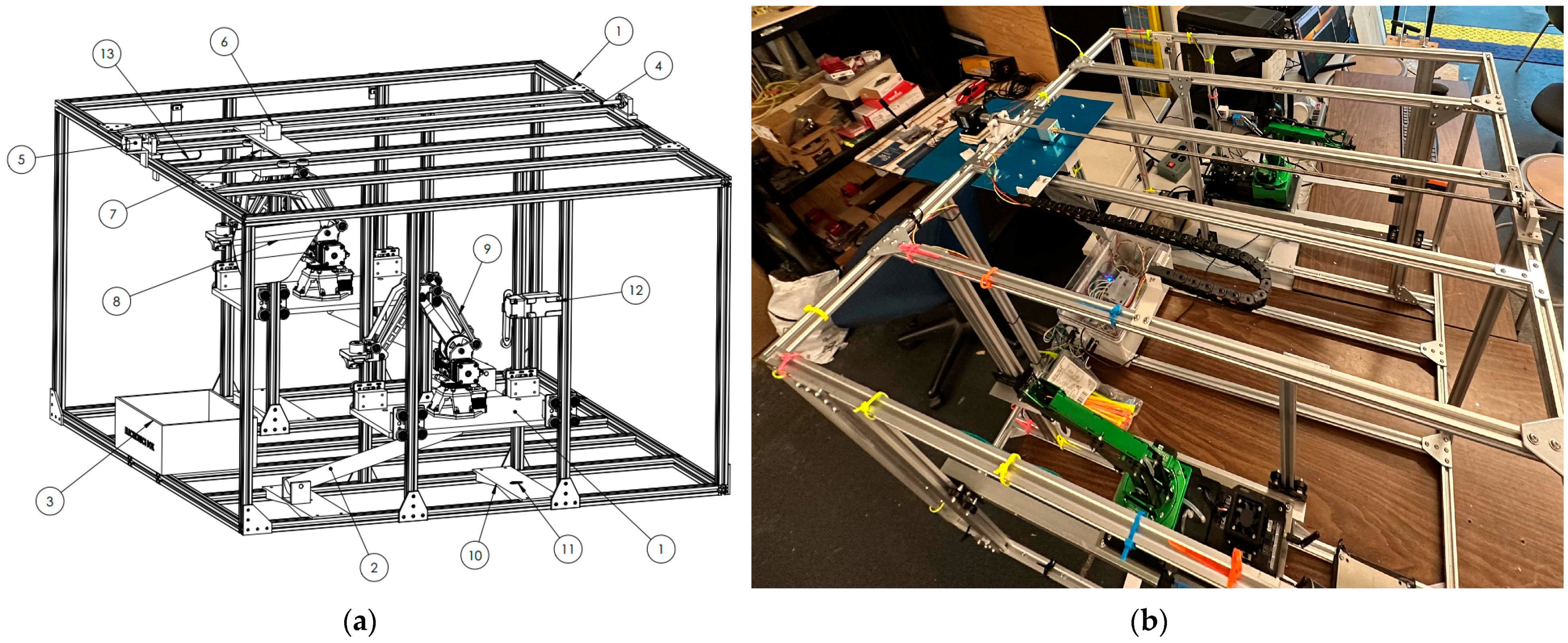
2. System Design and Prototyping
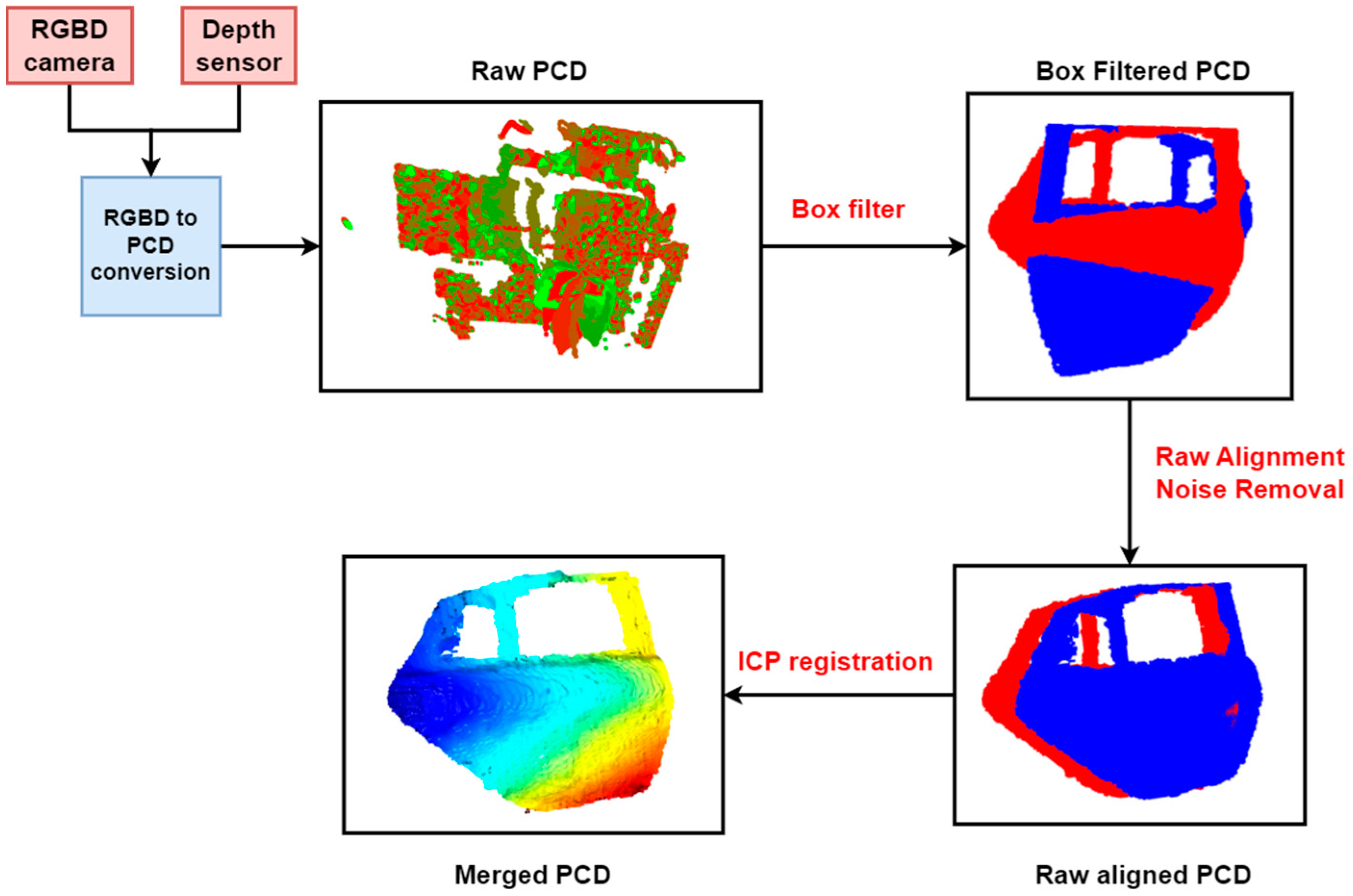
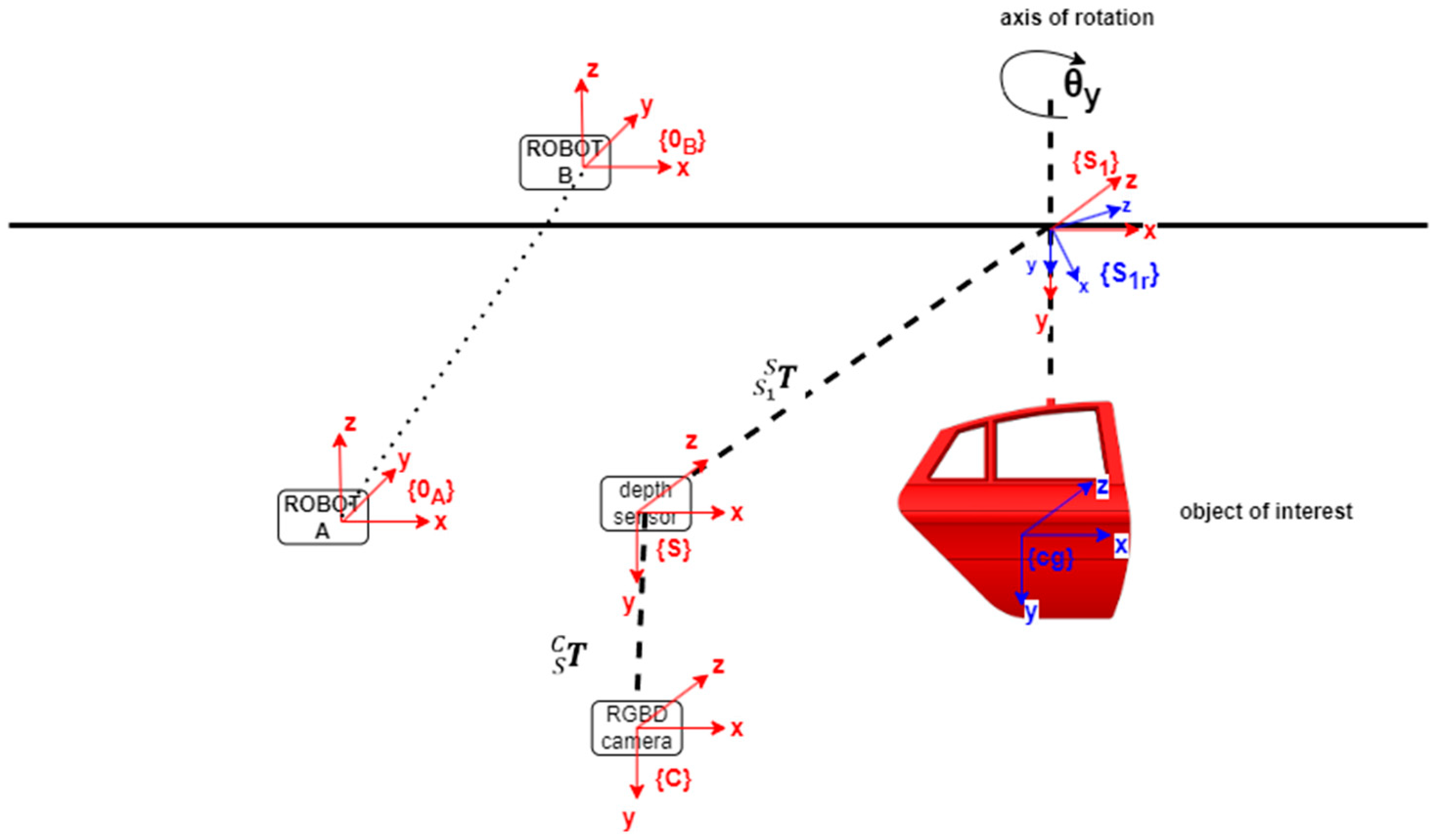
2.1. 3D Scanner and Calibrator
| Algorithm 1: ICP fine alignment |
| Input: (Raw aligned point clouds for each index ). (# of point clouds) Output: (Merged point cloud in the frame {C})
|
2.2. Optimal Trajectory Planner
2.3. Integrated System
3. Software Development
3.1. Software Framework
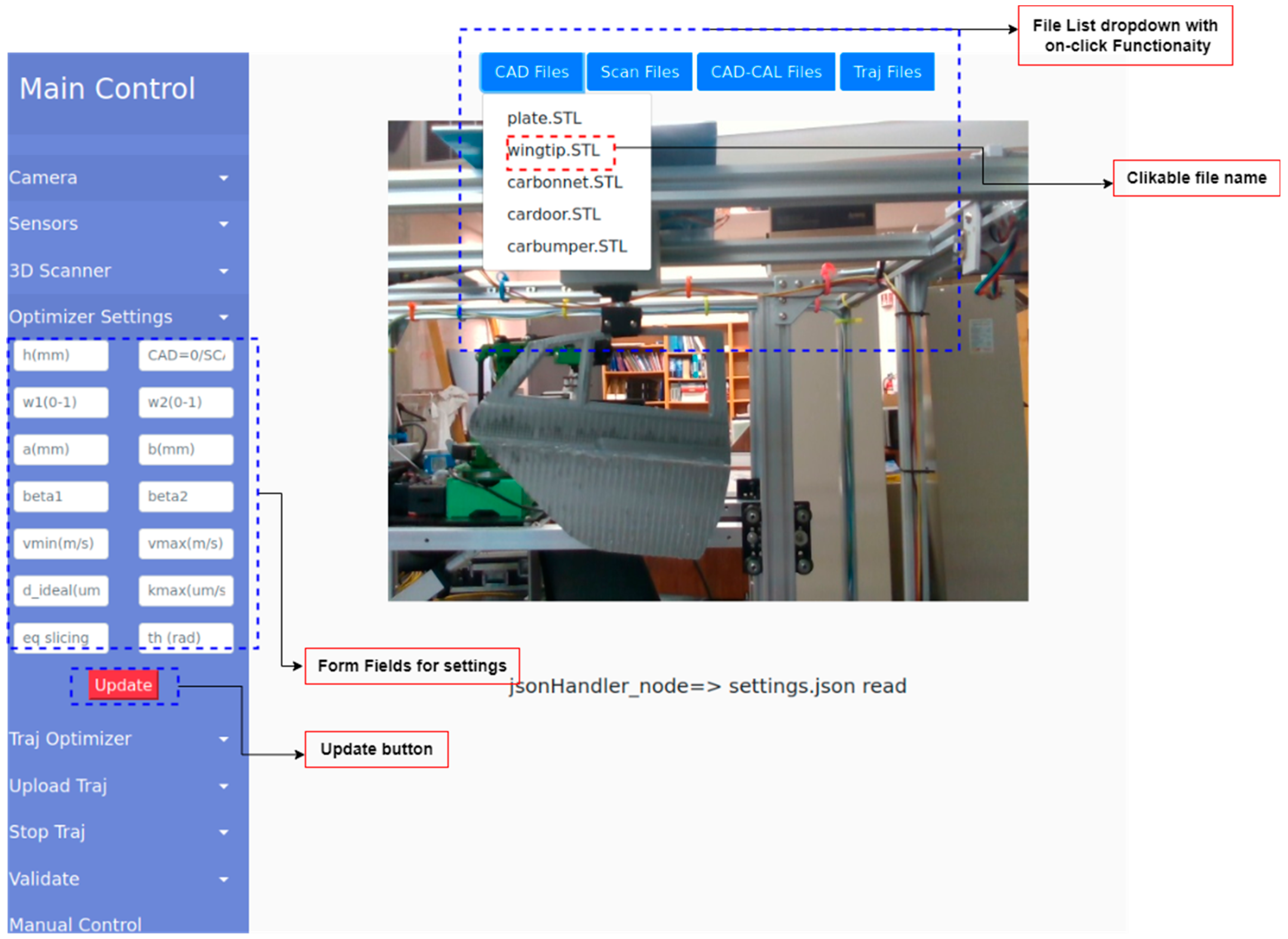
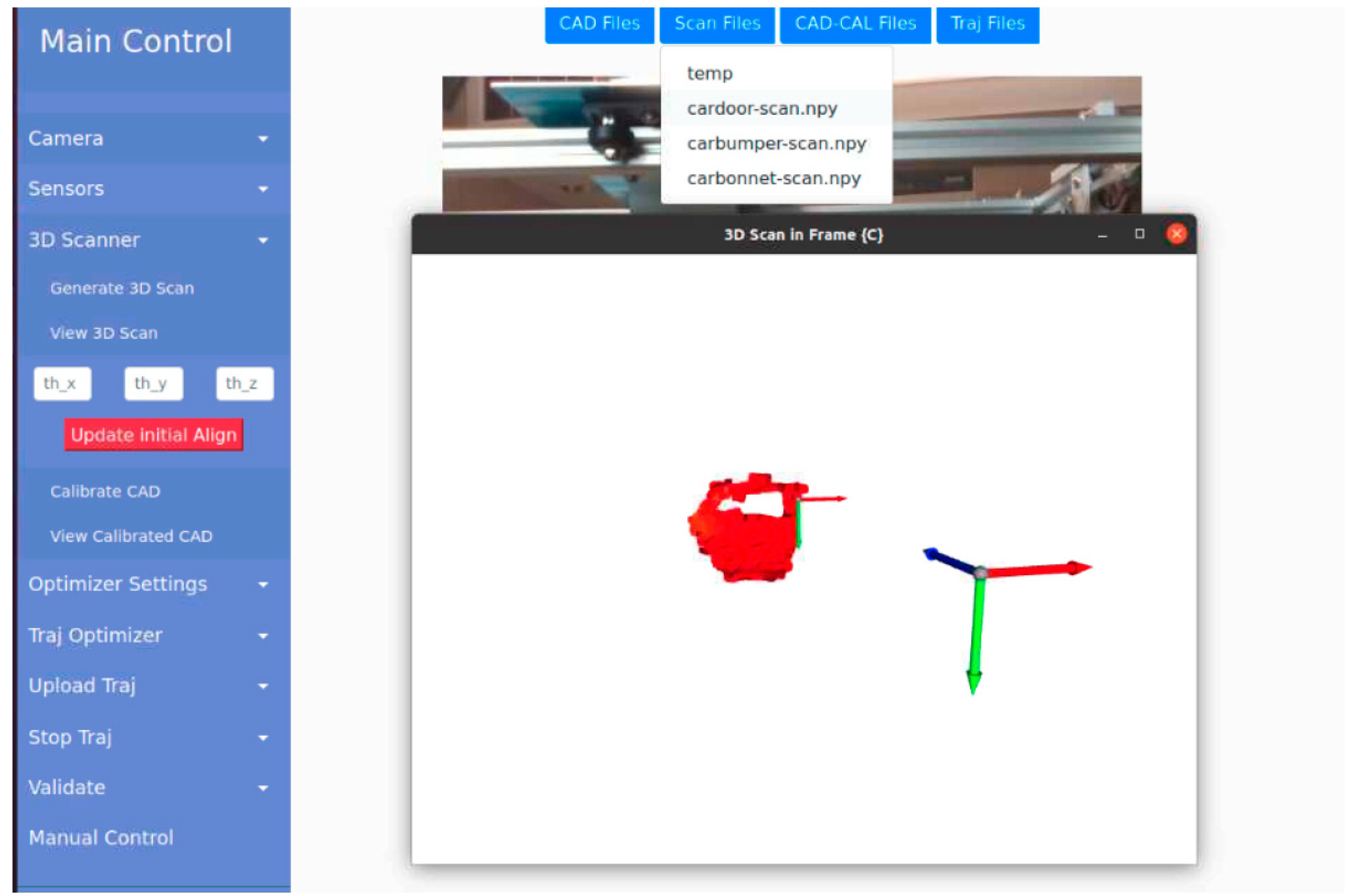
3.2. Graphical User Interface
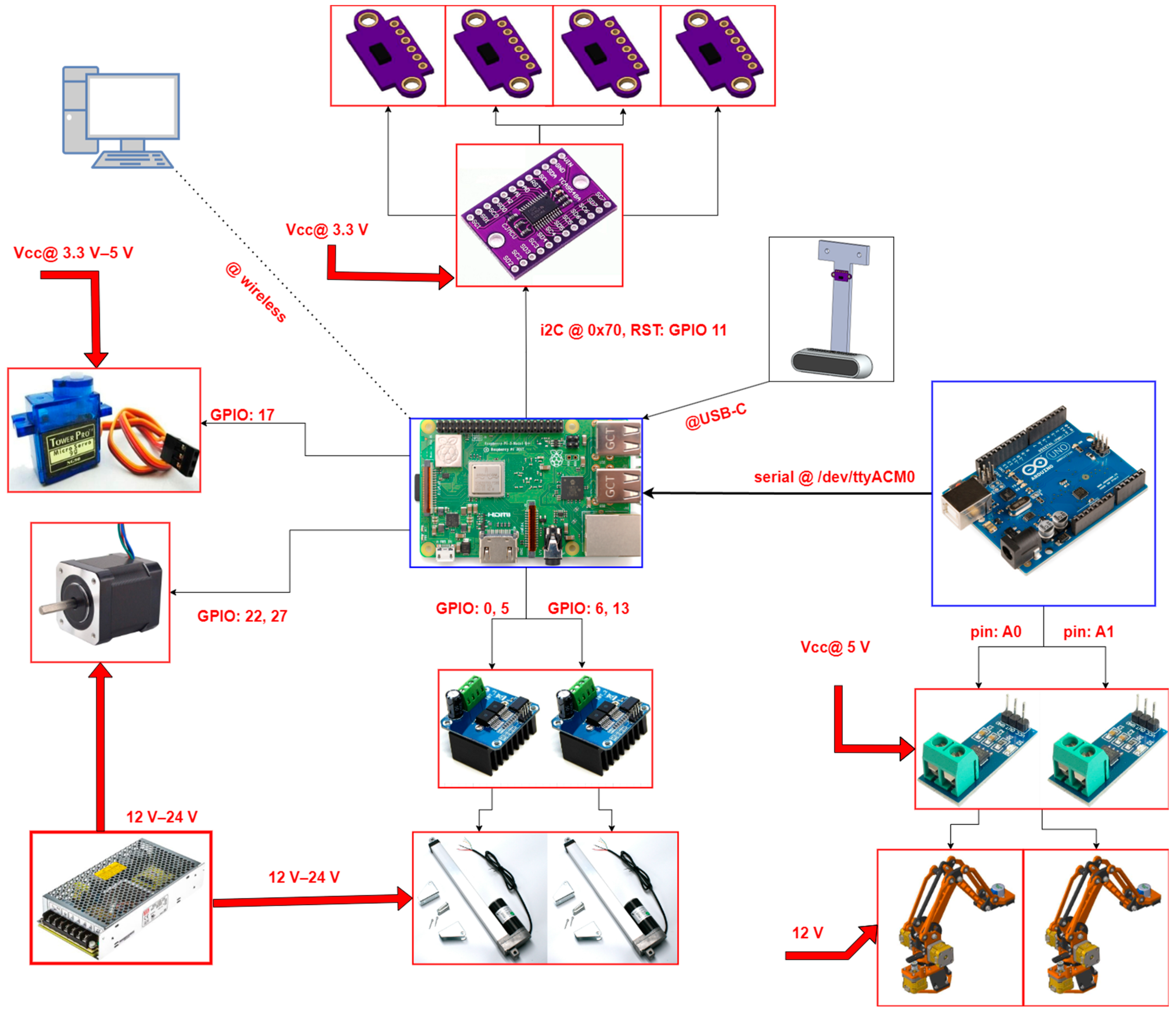
3.3. Circuit Connection Diagram
4. Results and Discussions
4.1. 3D Scanning and CAD Calibration
4.2. Optimal Trajectory Planning
4.3. Comparison with State of the-Art
5. Conclusions and Future Work
- A low-cost 3D scanner and calibrator that capture complex free-form surfaces with accuracies of up to 95%.
- An efficient trajectory planning scheme with energy savings of up to 73% and time savings of up to 33%.
- A trajectory planner capable of achieving optimal coating quality with relative coating errors as low as 5% and deviation errors as low as 17%.
- An easily scalable autonomous hardware–software framework using open-source software such as ROS and Python.
- An interactive web-based graphical user interface providing user control over the system and real-time monitoring of camera feeds, power consumption, and sensor states.
6. Patents
Author Contributions
Funding
Institutional Review Board Statement
Informed Consent Statement
Data Availability Statement
Acknowledgments
Conflicts of Interest
Appendix A

References
- KPMG. Global Automotive Executive Survey; Technical Report; KPMG: Amstelveen, The Netherlands, 2017. [Google Scholar]
- United States Environmental Protection Agency. Volatile Organic Compounds’ Impact on Indoor Air Quality. Available online: https://www.epa.gov/indoor-air-quality-iaq/volatile-organic-compounds-impact-indoor-air-quality#:~:text=Health%20effects%20may%20include%3A,kidney%20and%20central%20nervous%20system (accessed on 1 November 2023).
- Qlayers. Gone to Waste: Exploring the Environmental Consequences of Industrial Paint Pollution. Available online: https://www.qlayers.com/blog/gone-to-waste-exploring-the-environmental-consequences-of-industrial-paint-pollution (accessed on 1 November 2023).
- Bambousek, G.J.; Bartlett, D.S.; Schmidt, T.D. Spray Paint System including Paint Booth, Paint Robot Apparatus Movable Theren and Rail Mechanism for Supporting the Apparatus Thereout. U.S. Patent 4,630,567, 23 December 1986. [Google Scholar]
- Suh, S.-S.; Lee, J.-J.; Choi, Y.-J.; Lee, S.-K. A Prototype Integrated Robotic Painting System: Software and Hardware Development. In Proceedings of the 1993 IEE/RSJ International Conference on Intelligent Robots and Systems, Yokohama, Japan, 26–30 July 1993. [Google Scholar]
- Arıkan, M.A.S.; Balkan, T. Process Modeling, Simulation, and Paint Thickness Measurement for Robotic Spray Painting. J. Field Robot. 2000, 17, 479–494. [Google Scholar]
- Javaid, M.; Haleem, A.; Pratap, S.; Suman, R. Industrial perspectives of 3D scanning: Features, roles and it’s analytical applications. Sens. Int. 2021, 2, 100114. [Google Scholar] [CrossRef]
- Du, L.; Lai, Y.; Luo, C.; Zhang, Y.; Zheng, J.; Ge, X.; Liu, Y. E-quality Control in Dental Metal Additive Manufacturing Inspection Using 3D Scanning and 3D Measurement. Front. Bioeng. Biotechnol. 2020, 8, 1038. [Google Scholar] [CrossRef]
- Dombroski, C.E.; Balsdon, M.E.R.; Froats, A. The use of a low cost 3D scanning and printing tool in the manufacture of custom-made foot orthoses: A preliminary study. BMC Res. Notes 2014, 7, 443. [Google Scholar] [CrossRef]
- Yao, A.W.L. Applications of 3D scanning and reverse engineering techniques for quality control of quick response products. Int. J. Adv. Manuf. Technol. 2005, 26, 1284–1288. [Google Scholar] [CrossRef]
- Newcombe, R.A.; Izadi, S.; Hilliges, O.; Molyneaux, D. KinectFusion: Real-Time Dense Surface Mapping and Tracking. In Proceedings of the 10th IEEE International Symposium on Mixed and Augmented Reality, Basel, Switzerland, 26–29 October 2011. [Google Scholar]
- Meister, S.; Izadi, S.; Kohli, P.; Hammerle, M.; Rother, C.; Kondermann, D. When Can We Use KinectFusion for Ground Truth Acquisition? In Proceedings of the Workshop on Color-Depth Camera Fusion in Robotics, Daejeon, Repubic of Korea, 5–9 November 2012. [Google Scholar]
- Ma, F.; Carlone, L.; Ayaz, U.; Karaman, S. Sparse depth sensing for resource-constrained robots. Int. J. Robot. Res. 2019, 38, 935–980. [Google Scholar] [CrossRef]
- Larsson, S.; Kjellander, J.A. Motion control and data capturing for laser scanning with an industrial robot. Robot. Auton. Syst. 2006, 54, 453–460. [Google Scholar] [CrossRef]
- Borangiu, T.; Dumitrache, A. Robot Arms with 3D Vision Capabilities. In Advances in Robot Manipulators; IntechOpen: Rijeka, Croatia, 2010. [Google Scholar]
- Li, J.; Chen, M.; Jin, X.; Chen, Y.; Dai, Z.; Ou, Z.; Tang, Q. Calibration of a multiple axes 3-D laser scanning system consisting of robot, portable laser scanner and turntable. Optik 2011, 122, 324–329. [Google Scholar] [CrossRef]
- Pichler, A.; Viiicze, H.; Andersen, H.; Hladseii, O. A Method for Automatic Spray Painting of Unknown Parts. In Proceedings of the International Conference on Robotics & Automation, Washington, DC, USA, 11–15 May 2002. [Google Scholar]
- Andulkar, M.V.; Chiddarwar, S.S. Incremental approach for trajectory generation of spray painting robot. Ind. Robot. Int. J. 2015, 42, 228–241. [Google Scholar] [CrossRef]
- Chen, W.; Tang, Y.; Zhao, Q. A novel trajectory planning scheme for spray painting robot with Bézier curves. In Proceedings of the Chinese Control and Decision Conference (CCDC), Yinchuan, China, 28–30 May 2016; pp. 6746–6750. [Google Scholar]
- Yu, X.; Cheng, Z.; Zhang, Y.; Ou, L. Point cloud modeling and slicing algorithm for trajectory planning of spray painting robot. Robotica 2021, 39, 2246–2267. [Google Scholar] [CrossRef]
- Guan, L.; Chen, L. Trajectory planning method based on transitional segment optimization of spray transitional segment optimization of spray. Ind. Robot. Int. J. Robot. Res. Appl. 2019, 46, 31–43. [Google Scholar] [CrossRef]
- KUKA. KUKA Ready2_Spray. Available online: https://pdf.directindustry.com/pdf/kuka-ag/kuka-ready2-spray/17587-748199.html (accessed on 5 November 2023).
- FANUC. FANUC P-250iB Paint Robot. Available online: https://www.fanucamerica.com/products/robots/series/paint/p-250ib-paint-robot (accessed on 5 November 2023).
- ABB. IRB 5500-22/23. Available online: https://new.abb.com/products/robotics/industrial-robots/irb-5500-22 (accessed on 5 November 2023).
- RoboDK. Simulate Robot Applications. Available online: https://robodk.com/examples%7B#}examples-painting (accessed on 5 November 2023).
- Robotic and Automated Workcell Simulation, Validation and Offline Programming. Available online: www.geoplm.com/knowledge-base-resources/GEOPLM-Siemens-PLM-Tecnomatix-Robcad.pdf (accessed on 11 November 2023).
- Delfoi. Delfoi PAINT. Available online: https://www.delfoi.com/delfoi-robotics/delfoi-paint/ (accessed on 11 November 2023).
- ABB. RobotStudio® Painting PowerPac. Available online: https://new.abb.com/products/robotics/application-software/painting-software/robotstudio-painting-powerpac (accessed on 12 November 2023).
- Inropa™ OLP Automatic. Available online: https://www.inropa.com/fileadmin/Arkiv/Dokumenter/Produktblade/OLP_automatic.pdf (accessed on 14 November 2023).
- FANUC. FANUC ROBOGUIDE PaintPro. Available online: https://www.fanucamerica.com/support/training/robot/elearn/fanuc-roboguide-paintpro (accessed on 14 November 2023).
- Idrees, M.; Gabbar, H.A. A hybrid optimization scheme for efficient trajectory planning of a spray-painting robot. In Proceedings of the 3rd International Conference on Robotics, Automation, and Artificial Intelligence (RAAI), Singapore, 14–16 December 2023. [Google Scholar]
- IntelRealSense. Depth Camera D435. Available online: https://www.intelrealsense.com/depth-camera-d435/ (accessed on 15 November 2023).
- TowerPro. SG90 Digital. Available online: https://www.towerpro.com.tw/product/sg90-7/ (accessed on 15 November 2023).
- Davies, E.R. Machine Vision Theory, Algorithms, Practicalities; Elsevier: San Francisco, CA, USA, 2005. [Google Scholar]
- Zhou, Q.-Y.; Park, J.; Koltun, V. Open3D: A Modern Library for 3D Data Processing. In Proceedings of the Computer Vision and Pattern Recognition, Salt Lake City, UT, USA, 18–22 June 2018. [Google Scholar]
- Besl, P.; McKay, N.D. A method for registration of 3-D shapes. IEEE Trans. Pattern Anal. Mach. Intell. 1992, 14, 239–256. [Google Scholar] [CrossRef]
- Amazon. Nema 23 Stepper Motor Bipolar 1.8 Degree 2.8A. Available online: https://www.amazon.com/JoyNano-Nema-23-Stepper-Motor/dp/B07H866S2F?th=1 (accessed on 18 November 2023).
- Hiwonder. Jetmax Jetson Nano. Available online: https://www.hiwonder.com/products/jetmax?variant=39645677125719 (accessed on 18 November 2023).
- ESPHome. VL53L0X Time of Flight Distance Sensor. Available online: https://esphome.io/components/sensor/vl53l0x.html (accessed on 18 November 2023).
- Amazon. Electrical Buddy Adjustable Rod Lever Arm Momentary Limit Switch. Available online: https://www.amazon.ca/Electrical-Buddy-Adjustable-Momentary-Me-8107/dp/B07Y7C9188 (accessed on 19 November 2023).
- Quigley, M.; Gerkey, B.; Conley, K.; Faust, J.; Foote, T.; Leibs, J.; Berger, E.; Wheeler, R.; Ng, A. ROS: An open-source Robot Operating System. In Proceedings of the ICRA Workshop on Open Source Software, Kobe, Japan, 12–17 May 2009. [Google Scholar]
- JavaScript. Pluralsight. Available online: https://www.javascript.com/ (accessed on 20 November 2023).
- Bootstrap. Available online: https://getbootstrap.com/docs/4.2/getting-started/introduction/ (accessed on 21 November 2023).
- The Standard ROS JavaScript Library. ROS.org. Available online: https://wiki.ros.org/roslibjs (accessed on 21 November 2023).
- van Rossum, G.V. Python. Available online: https://www.python.org/ (accessed on 24 November 2023).
- Osada, R.; Funkhouser, T.; Chazelle, B.; Dobkin, D. Matching 3D models with shape distributions. In Proceedings of the International Conference on Shape Modeling and Applications, Genova, Italy, 7–11 May 2001; pp. 154–166. [Google Scholar]


| ID | Component Description | CAD Model |
|---|---|---|
| 1 | Aluminum framing used for building the structure of the entire system. It also contains corner brackets, T-brackets, and gantries for achieving smooth linear motion. | 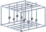 |
| 2 | Vertical sliding mechanism. It contains two linear actuators, a support base for lifting the robots, and a base mount plate for securing the linear actuators. For position feedback, VL53L0X sensors are installed. These actuators are used for extended reach in case of large objects. | 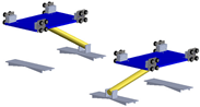 |
| 3 | Electronics box for keeping the electrical components. It contains a Raspberry Pi controller, an Arduino, two motor controllers for the linear actuators, current sensors, and a stepper driver. The choice of Raspberry Pi controller is due to its low cost and easy integration with the ROS ecosystem, while Arduino is used for its easy to access a DAC (Digital-to-Analog Convertor). | 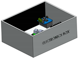 |
| 4 | Horizontal sliding mechanism. It contains a threaded rod, two guide rails with linear gantries, bearings and bearing supports for the threaded rod, a stepper motor for driving the mechanism, and a distance feedback sensor. |  |
| 5 | Stepper motor [37] for moving the horizontal slider. This motor is a suitable choice for the system due to its easy availability, high torque for a low price, and convenient integration with the Raspberry Pi. |  |
| 6 | Horizontal slider jockey. It contains a lead screw head connected to the base plate, which is then connected to the linear gantries for moving along the guide rails. | 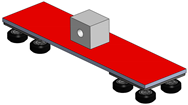 |
| 7 | Rotating servomechanism for 3D scanner. The servomechanism [33] is connected to the object via a gripper that can be tightened and loosened. The object is a car door, as illustrated in the CAD. |  |
| 8 | A downscaled CAD model of a car door for 3D scanning and trajectory planning. |  |
| 9 | Two 3-DOF Jetmax robots for controlling the x, y, and z locations of the end effector [38]. The robot combined with the vertical sliding mechanism gives a total of 4 DOF for executing the trajectory over the surface of a complex free-form surface (e.g., car door). The choice of a Jetmax robot is due to its low price and convenient integration with the ROS ecosystem. | 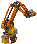 |
| 10 | Position feedback platform for the linear actuators with distance feedback sensor. | 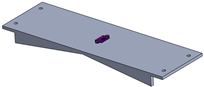 |
| 11 | VL53L0X sensor [39]. It is a time-of-flight (TOF) sensor for measuring distance. It has a measurement range of and an accuracy of These sensors are more accurate and precise than SONAR (Sound Navigation and Ranging) sensors, which makes them a good choice for the integrated system. |  |
| 12 | A limit switch used for disconnecting the power from the linear actuators [40]. | 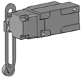 |
| 13 | 3D scanning hardware, including an Intel Real Sense D435 sensor [32] and a VL53L0X sensor for axis calibration. These sensors are low-cost compared to laser scanners, which makes them a suitable choice for the integrated system. | 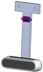 |
| Parameter | Description | Value |
|---|---|---|
| Spraying process parameters | ||
| Ellipse longer side for the coating model | ||
| Ellipse shorter side for the coating model | ||
| Coating distribution beta along the X direction of ellipse | ||
| Coating distribution beta along the Y direction of ellipse | ||
| Coating deposition rate | ||
| Desired coating thickness | ||
| Minimum speed of the spray gun | ||
| Maximum speed of the spray gun | ||
| Spray gun height from the surface | ||
| Robot model parameters | ||
| Link 0 stroke length | ||
| Manipulator Link 1 length | ||
| Manipulator Link 2 length | ||
| Manipulator Link 3 length | ||
| Manipulator Link 0 mass | ||
| Manipulator Link 1 mass | ||
| Manipulator Link 2 mass | ||
| Manipulator Link 3 mass | ||
| Optimizer Parameters | ||
| Scaling factor for mean-squared error | ||
| Scaling factor for coating deviation error | ||
| Scaling factor for mean energy consumption | ||
| Scaling factor for mean trajectory time | ||
| Hyper-parameter in the fitness function | ||
| Mutation rate in GA | ||
| Crossover type in GA | Two points | |
| Mutation type in GA | Random | |
| Number of mating parents in GA | ||
| Number of generations in GA | ||
| Number of solutions per population in GA |
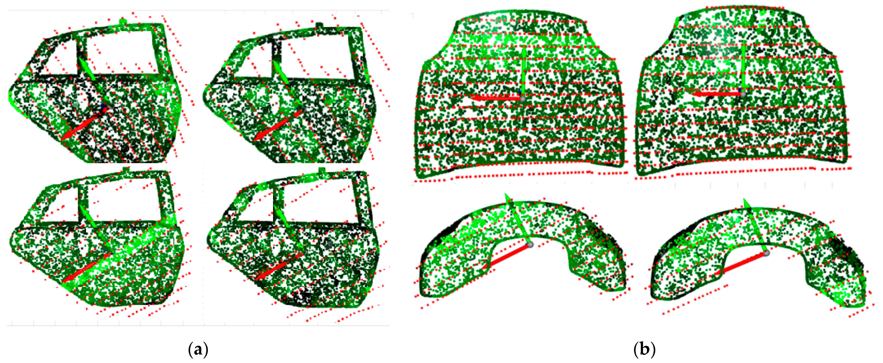
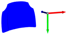
| Scanned Geometry in Frame {C} | Calibrated CAD in Frame {C} |
|---|---|
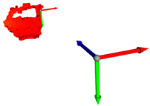 |  |
 |  |
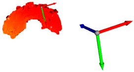 | 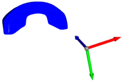 |
| D1 Score | D2 Score | Avg Score | |
|---|---|---|---|
| Car door | 0.9639 | 0.9434 | 0.9536 |
| Car hood | 0.9524 | 0.9228 | 0.9376 |
| Car bumper | 0.9488 | 0.9082 | 0.9285 |
| Slicing Scheme | Experimental | Theoretical | Experimental | ||
|---|---|---|---|---|---|
| Car door | Non-equidistant | 90° | 2085 J | 60% | 44% |
| Equidistant (ref.) | 30° | 3003 J | 0% | 0% | |
| Car hood | Non-equidistant | 90° | 1569 J | 73% | 51% |
| Equidistant (ref.) | 0° | 3212 J | 0% | 0% | |
| Car bumper | Non-equidistant | 90° | 1275 J | 64% | 33% |
| Equidistant (ref.) | 0° | 1894 J | 0% | 0% |
| Article | U-Direction [19] | V-Direction [19] | Equidistant Slicing [20] | Non. Eq Slicing [20] | Transitional- Seg Opt [21] | Proposed Scheme | Proposed Scheme | Proposed Scheme |
|---|---|---|---|---|---|---|---|---|
| Object of interest | Oval Bucket | Oval Bucket | Motorcycle spoiler | Motorcycle spoiler | Aircraft wing | Car door | Car hood | Car bumper |
| Desired coating thickness | ||||||||
| Mean coating thickness | ||||||||
| Standard deviation | ||||||||
| Mean coating deviation error | ||||||||
| Mean relative coating error | ||||||||
| Max time savings | N/A | N/A | N/A | |||||
| Max energy savings | N/A | N/A | N/A | N/A | N/A | |||
| Coating mean-squared error cost | Yes | Yes | Yes | Yes | Yes | Yes | Yes | Yes |
| Coating deviation cost | No | No | No | No | No | Yes | Yes | Yes |
| Energy cost | No | No | No | No | No | Yes | Yes | Yes |
| Process time cost | No | No | No | No | No | Yes | Yes | Yes |
Disclaimer/Publisher’s Note: The statements, opinions and data contained in all publications are solely those of the individual author(s) and contributor(s) and not of MDPI and/or the editor(s). MDPI and/or the editor(s) disclaim responsibility for any injury to people or property resulting from any ideas, methods, instructions or products referred to in the content. |
© 2024 by the authors. Licensee MDPI, Basel, Switzerland. This article is an open access article distributed under the terms and conditions of the Creative Commons Attribution (CC BY) license (https://creativecommons.org/licenses/by/4.0/).
Share and Cite
Gabbar, H.A.; Idrees, M. ARSIP: Automated Robotic System for Industrial Painting. Technologies 2024, 12, 27. https://doi.org/10.3390/technologies12020027
Gabbar HA, Idrees M. ARSIP: Automated Robotic System for Industrial Painting. Technologies. 2024; 12(2):27. https://doi.org/10.3390/technologies12020027
Chicago/Turabian StyleGabbar, Hossam A., and Muhammad Idrees. 2024. "ARSIP: Automated Robotic System for Industrial Painting" Technologies 12, no. 2: 27. https://doi.org/10.3390/technologies12020027
APA StyleGabbar, H. A., & Idrees, M. (2024). ARSIP: Automated Robotic System for Industrial Painting. Technologies, 12(2), 27. https://doi.org/10.3390/technologies12020027