Abstract
When training a parametric surrogate to represent a real-world complex system in real time, there is a common assumption that the values of the parameters defining the system are known with absolute confidence. Consequently, during the training process, our focus is directed exclusively towards optimizing the accuracy of the surrogate’s output. However, real physics is characterized by increased complexity and unpredictability. Notably, a certain degree of uncertainty may exist in determining the system’s parameters. Therefore, in this paper, we account for the propagation of these uncertainties through the surrogate using a standard Monte Carlo methodology. Subsequently, we propose a novel regression technique based on optimal transport to infer the impact of the uncertainty of the surrogate’s input on its output precision in real time. The OT-based regression allows for the inference of fields emulating physical reality more accurately than classical regression techniques, including advanced ones.
1. Introduction
In any scientific domain, a system can be subjected to various sources of uncertainties, whether aleatoric, resulting from the inherent randomness of reality, or epistemic, arising from a lack of knowledge. In this context, uncertainty quantification (UQ) can be defined as the end-to-end study of the reliability of science inference [1]. This entails an examination of the relationship between approximate pieces of information regarding reality or, in simpler terms, the sensitivity of the analysis output to variations in the governing assumptions. UQ analyzes uncertainties within mathematical models, simulations, and data, quantifying how they propagate from input variables to the distribution of the final output in a system or model. It aims to assess the reliability of predictions and consider the impacts of variability and randomness in models. Consequently, UQ is playing an increasingly critical role in various tasks, including sensitivity analysis, design with uncertainty, reliability analysis, risk evaluation, and decision-making, becoming an indispensable tool across diverse engineering fields [2].
Today, the development of a vast majority of fields relies on predictions derived from data-driven models. Indeed, in the late 20th century, models based on data gained widespread development. These metamodels, also identified as parametric surrogates, serve as representations of real-world systems with all the complexity, ensuring real-time constraints without necessitating insights into the actual physics of the asset [3,4,5,6,7,8]. Consequently, they facilitate real-time monitoring and control of the most pertinent physical quantities of the system, enabling intelligent decision-making and optimization.
Real-time surrogates are of significant interest in both industrial applications and research. These tools, employing regression techniques, enable the exploration of the parametric space of a problem in an online manner, eliminating the need for expensive and time-consuming numerical or experimental evaluations. However, they also present certain challenges and considerations. First, they need an offline training stage, which can be time-consuming, along with a training data set whose quality is crucial for the accuracy of the trained surrogate. Additionally, the choice of the surrogate’s architecture plays a fundamental role in achieving precise predictions and ensuring the tool’s operational efficiency, particularly in cases with limited computing power. Lastly, with the increasing complexity of the surrogates’ model design, the interpretability and understandability of the model become essential.
However, modeling a complex system involves the characterization of some inputs that may carry uncertainties, such as material properties and initial or boundary conditions. Despite the comprehensible and coherent evolution of nature, a level of physical variability should always be considered, introducing uncertainty into any real process and its corresponding model. Additionally, data uncertainty may arise during the measurement of a system’s features, independent of its inherent variability. This uncertainty can be related to factors such as measurement population sampling, measurement methodology, or imperfections in the manufacturing process [9]. Therefore, Uncertainty Quantification (UQ) contributes to a deeper understanding of how models respond to changes in their input parameters.
Therefore, UQ endeavors to overcome the deterministic aspect inherent in data-driven modeling. Various statistical, computational, and mathematical methods are employed for this purpose, enabling the identification of the probabilistic distribution of data and its propagation through a system’s surrogate [10,11,12,13,14,15]. Notable methods among them include Monte Carlo methods [16], Polynomial Chaos Expansion [17,18], and Gaussian Processes [19].
This paper aims to delve into the propagation of uncertainty in a system through its data-driven metamodeling. In this context, we investigate how uncertainty in a system’s parameters propagates through its surrogate model. Therefore, we present a strategy to quantify the impact of input uncertainty on the precision of the trained parametric metamodel. When training a surrogate, we focus on maximizing the accuracy of the quantity of interest () inferred for a given set of input parameters with respect to its reference value. Here, we focus on evaluating the precision of the surrogate’s output, assuming uncertainty in its inputs once it is trained.
Therefore, within a parametric metamodeling framework, we can develop a data-based model that characterizes the uncertainty associated with the surrogate’s output. Specifically, for a trained surrogate representing the studied system, we introduce a data-based model that takes the definition of its input’s uncertainty as an input and provides a confidence interval (CI) of its output. In this context, certain descriptors of the input’s uncertainty are assumed to be known. The corresponding output’s uncertainty, represented by the CI, is computed using a standard Monte Carlo estimator approach.
The novelty presented in this paper lies in the creation of such a data-based model relying on optimal transport (OT) theory [20]. Leveraging this theory enables us to infer a CI for a surrogate’s output in real time when provided with an uncertainty descriptor for its input. This approach accurately emulates physical reality, benefiting from a conceptually different regression perspective offered by OT theory.
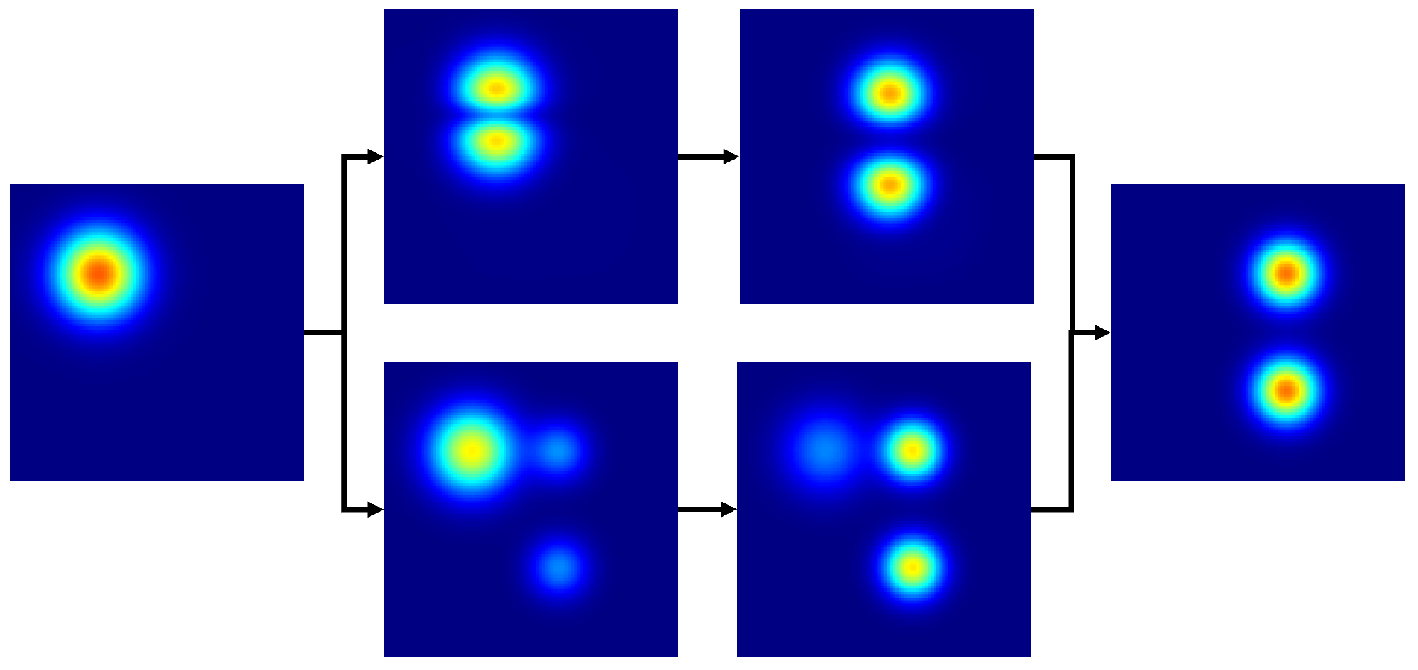
Regression, a foundational mathematical operation extensively applied in engineering, may yield non-physical results in certain fields, such as fluid dynamics, even with advanced classical techniques [21]. A smarter approach involves leveraging optimal transport theory, which offers a fundamentally distinct method for function interpolation, deemed more physically relevant in various domains. In contrast to conventional Euclidean interpolation, where a blend of two interpolated functions occurs with one progressively disappearing while the other appears, OT-based interpolation involves gradual translation and scaling, as illustrated in Figure 1. This solution is more realistic in fields like fluid dynamics and computer vision, justifying its widespread use. In this context, optimal transport quantifies the distance between functions by identifying the most cost-effective way to transform all mass units describing one function into the shape of another [22]. However, the computational cost associated with computing optimal transport presents a challenge. Despite recent advances in solving it [23,24], the problem remains inaccessible for real-time applications.
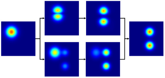
Figure 1.
Interpolated function is depicted for different t values, spanning from to , utilizing the optimal transport approach (Top) and the classic interpolation method with associated spurious effects (Bottom). Notably, when inferring the 2-dimensional solutions between the fields and , OT provides a solution that can be considered much more realistic in various fields, such as fluid dynamics. Unlike the conventional Euclidean interpolation, which exhibits a blend of two interpolated functions with one progressively disappearing while the other appears, OT-based interpolation involves gradual translation and scaling.
The authors have previously explored such a regression solution, as detailed in a previous work [25], where it was employed to construct a surrogate for the studied system, overcoming the real-time accessibility issue. In this current paper, the same optimal transport regression technique is employed to model the confidence interval of the trained surrogate’s output, given descriptors of the input’s uncertainty. Therefore, we leverage the previously developed regression tool to establish an optimal transport-based parametric metamodel for this CI, with the parameters representing the descriptors of the input’s uncertainty.
In this article, we first introduce the uncertainty propagation methodology. Then, we present the key concepts of optimal transport theory along with the main steps of the OT-based regression methodology. Finally, we study some examples from various domains, including fluid and solid dynamics.
2. Uncertainty Propagation through Parametric Surrogate
In this section, we study the uncertainty propagation of a parameter of the studied system through the corresponding system’s surrogate. For this purpose, we introduce a system parameterized by d features denoted as . For such a system, we suppose the existence of a trained surrogate g, taking the d parameters as input and returning the in real time:
where denotes any associated with the system characterized by within its corresponding space . To train this surrogate during an offline phase, a Design of Experiment () is established based on the system’s parameters, and the corresponding system’s responses are compiled in a training database. These responses may be obtained through numerical simulations or experimental measurements.
The surrogate is subsequently trained employing Machine Learning and Model Order Reduction techniques [26,27,28,29,30,31]. It is important to emphasize that during the surrogate training process, we assume precise knowledge of the values of each feature in . This assumption enables the collection of the corresponding quantity of interest for the parameters’ samples within the . Consequently, once it is trained, the surrogate can efficiently infer the quantity of interest associated with any possible value of in real time.
We now introduce uncertainty into the features of the system. Specifically, we suppose that each parameter , follows a normal distribution with mean and variance , denoted as . Assuming all are independent:
The objective at this stage is to relate the descriptors defining the uncertainty of the features and the uncertainty associated with the quantity of interest . This can be understood as learning estimators for the average M and variance of the quantity of interest, given any choice of and . This relationship is established through two parametric data-based models, respectively:
where and are the estimators of the average and variance of the quantity of interest, respectively.
To train these data-based models, a training data set comprising points is required:
which can be generated through a Monte Carlo sampling strategy. It is important to note that the architecture of these parametric data-based models follows the OT-based regression technique developed by the authors [25], which is further presented in detail later in this paper.
After training the OT-based models, it becomes possible to infer a real-time confidence interval for the surrogate’s output concerning new uncertainty descriptors for the system parameters. This involves a new parameter set denoted as corresponding to .
The coefficient follows a Student’s t distribution. Its choice depends on the desired confidence level: a higher value of the coefficient corresponds to a greater desired confidence level, indicating a reduced risk of inaccuracies in predictions assumed. A commonly adopted choice across various fields is for a confidence level of .
The procedure for training the data-based models of the estimators is outlined in Algorithm 1. It is noteworthy that the surrogate of the system is called multiple times, underscoring the necessity for a surrogate that is accessible in real time. Moreover, note that the accuracy error of the system’s surrogate is not considered. Indeed, we assume that this error is small in absolute terms and in comparison with the variability introduced by the Monte Carlo sampling in the system’s output.
| Algorithm 1: Estimators Data-based Models Based on Monte Carlo Sampling |
|
3. Revisiting Optimal Transport
In this section, we introduce the optimal transport framework and present the foundational tools upon which the subsequently developed OT-based parametric surrogate relies. It is important to note that this section provides a non-exhaustive overview of the key concepts in optimal transport. For further documentation on this subject, we encourage interested readers to refer to [32] and its associated references.
In the 18th century, the optimal transport theory was initially explored by Monge [33]. Driven by a military context, he delved into determining the most cost-effective method for transporting a specified quantity of soil from its source to construction sites. To introduce the OT-based regression technique, we will constrain the Monge discrete problem within a 2-dimensional convex domain.
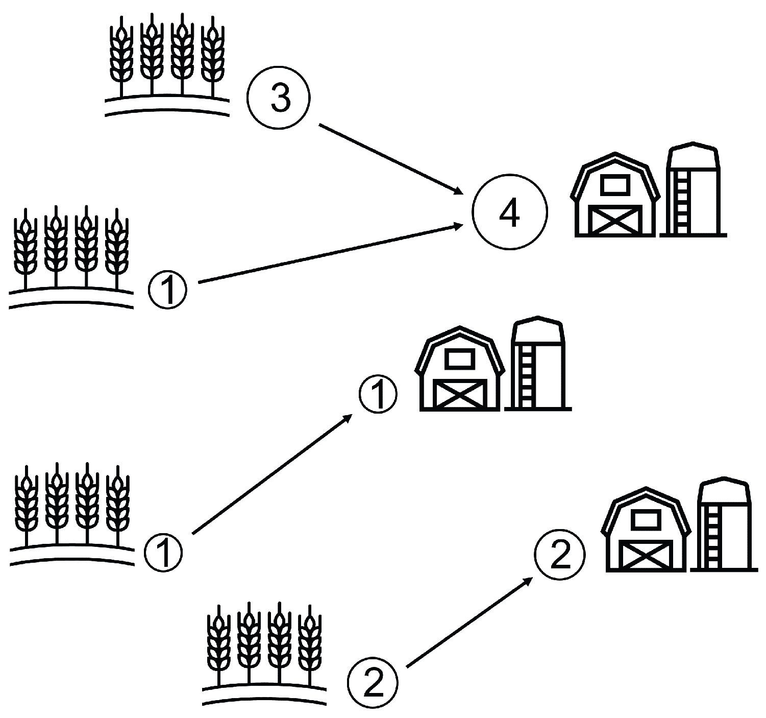
First, we present this optimal transport discrete problem by considering the transportation of wheat produced by W wheat fields to F farms, as schematized in Figure 2. The wheat must be optimally transported, minimizing the defined cost: the distance traveled.

Figure 2.
Optimal transport discrete Monge problem between wheat fields and farms. Each field produces a certain quantity of wheat: , , and . Each farm consumes a certain quantity of wheat: , and . The minimized cost is the square of the Euclidian distance.
We consider that each wheat field, indexed by (where represents the set ) and situated at , yields a wheat quantity of . Similarly, each farm, indexed by and located at , consumes a quantity of wheat. Introducing the concept of measure, the distributions of wheat produced by the fields, denoted as , and consumed by the farms, denoted as , can be defined as
where and represent the Dirac measures at positions and , respectively.
Therefore, the Monge problem involves finding an optimal map T that associates each location with a unique location . This map is required to transfer the produced wheat in the fields to the consumed wheat by the farms . Since no wheat can be created, destroyed, or divided during the transportation, this surjective map must satisfy the mass conservation
Furthermore, this map must minimize the cost function c, defined here as the square of the Euclidean norm of the distance traveled between the wheat field indexed by i and its corresponding farm indexed by j:
Hence, the resulting minimization problem writes:
The just presented Monge discrete problem is now simplified by introducing certain hypotheses for the development of the OT-based parametric surrogate. Indeed, the Monge minimization problem seeks the most cost-effective way to map the distributions of wheat produced by the fields and consumed by the farms. Likewise, we aim to find the most cost-effective way to map our functions. Upon discovering this mapping, we can utilize it to infer any new solutions between our functions.
First, we assume an equal number of wheat fields and farms: . Additionally, we consider that each wheat field produces an identical quantity of wheat, and each farm consumes the same quantity of wheat, i.e., . Consequently, the Monge discrete problem applies now between two discrete distributions featuring an equal number of points, with uniform weights assigned to each point.
As a result, the mass conservation constraint implies that the sought-after map T becomes a bijection, and the corresponding optimal transport minimization problem evolves into an optimal assignment problem between two 2-dimensional point clouds featuring the same number of points and uniform weights. Given the cost matrix , where , this optimal assignment problem aims to find the bijection T within the set of permutations of W elements, solving:
Thus, as illustrated in Figure 3, where each point is defined by its x and y coordinates, our objective is to find the bijection T between the red and blue clouds, minimizing the specified cost function: the square of the Euclidian distance between the assigned points. Such an optimal assignment problem can be efficiently addressed through Linear Programming.
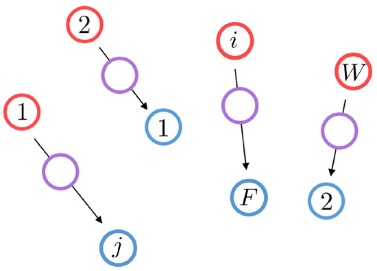
Figure 3.
Discrete Monge problem equivalent to an optimal assignment problem where and . Wheat fields are represented by red circles, and farms by blue ones. The optimal matching is illustrated by black arrows. The interpolated distribution is depicted by violet points.
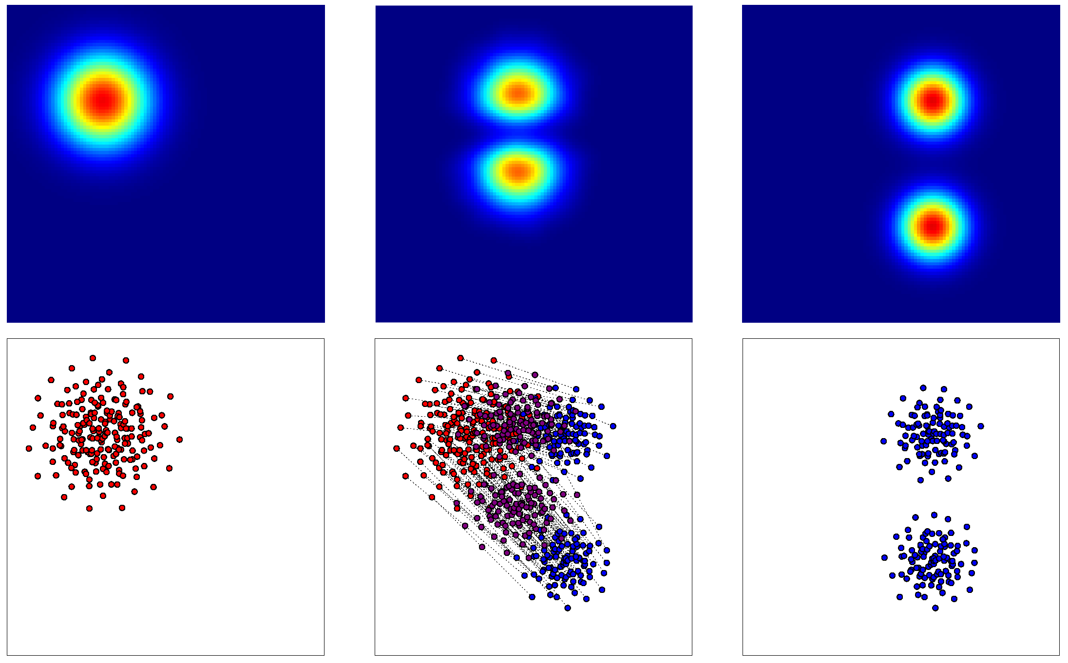
Upon solving the optimal matching between the two point clouds, it becomes feasible to interpolate between the two distributions in an optimal transport manner. This process involves partially displacing all points along the corresponding segments formed between matched points. The resultant interpolated distribution, or point cloud, is depicted in Figure 3 by violet points. Therefore, we employ this discrete point cloud interpolation technique, relying on an optimal assignment, to interpolate between our functions. However, given that our functions are continuous, we first decomposed them into a sum of identical Gaussian functions, leading to discrete point clouds that we can work with, as presented thereafter.
4. Learning Surrogate’s Output Variability with Optimal Transport
The regression technique based on optimal transport, developed by the authors and published in [25], is shortly reviewed here. For a comprehensive understanding of its implementation, we strongly recommend that interested readers consult the aforementioned publication for all the details.
Our objective is to develop a regression technique capable of inferring any possible solution within a parametric space, utilizing the optimal transport theory. For this purpose, we leverage the discrete Monge problem, which has been simplified based on the previously presented hypotheses. Hence, employing this Lagrangian formulation of the problem and displacement interpolation [34], the developed method addresses the regression problem as an optimal assignment problem, such as the one represented in Figure 3. The paths followed by each point are parameterized, providing access to an interpolated solution by selectively displacing the points along these paths at specific parameter values.
Let us introduce a parametric problem defined in , where represent the parameters of the studied system. Next, we consider P samples in corresponding to the solutions of the problem. To introduce the OT-based parametric surrogate, but without loss of generality, we assume that each sample is a surface , where is the 2-dimensional physical domain of the problem. This choice is coherent with the cases studied and presented in the results section.
First, the OT-based model is trained in an offline stage as follows:
- 1.
- Pre-processing: Normalization of the surfaces to obtain unitary integral surfaces:
- 2.
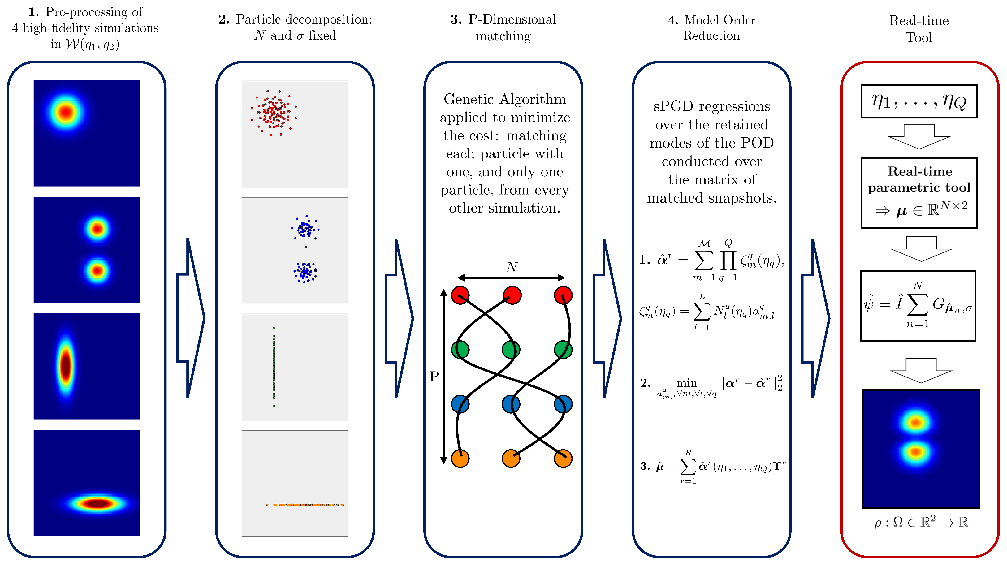
- Particles decomposition: Each surface is represented as a sum of N identical 2D-Gaussian functions, referred to as particles. These particles are characterized by a fixed standard deviation and a mass of . It should be highlighted that the number of particles N and the standard deviation for each particle constitute hyperparameters in our methodology.Hence, for a given surface, the only variables are the means of each Gaussian function, i.e., N vectors with 2 components each: and (because we are in 2 dimensions).Therefore, to determine the positions of the N particles, we need to solve P optimization problems (i.e., one for each surface) aimed at minimizing the error between the reconstructed surface and the original one. To solve each optimization problem, a Gradient Descent approach is employed:where M is the number of points of the mesh where the surface is represented.Once the decomposition is computed, the matrix , composed by the x and y coordinates of every particle of the surface , can be introduced:It is important to emphasize that the arrangement of particles in this matrix is not arbitrary; instead, it is utilized to account for the matching between point clouds. Specifically, the particle in the nth row for one cloud is paired with the particle in the nth row in every other cloud.
- 3.
- -dimensional matching: Once two surfaces, and , are decomposed into N particles, the optimal matching between the two clouds can be computed solving the optimal assignment problem. This involves minimizing the cost , as presented before, which is defined as the sum of the squared Euclidian distances between matched particles:where is a bijection within the set of permutations of N elements. The function assigns a new position to each particle n in the distribution p, considering the order within . Indeed, captures the arrangement of the N particles in the distribution p. The goal is to determine the optimal function , representing the most advantageous ordering that corresponds to the optimal matching, therefore minimizing the defined cost.Subsequently, as illustrated in Figure 4, it becomes feasible to interpolate between the two surfaces by reconstructing the surface after partially displacing all the particles along the respective segments formed between each particle from one surface and its corresponding optimal pair on the other surface.
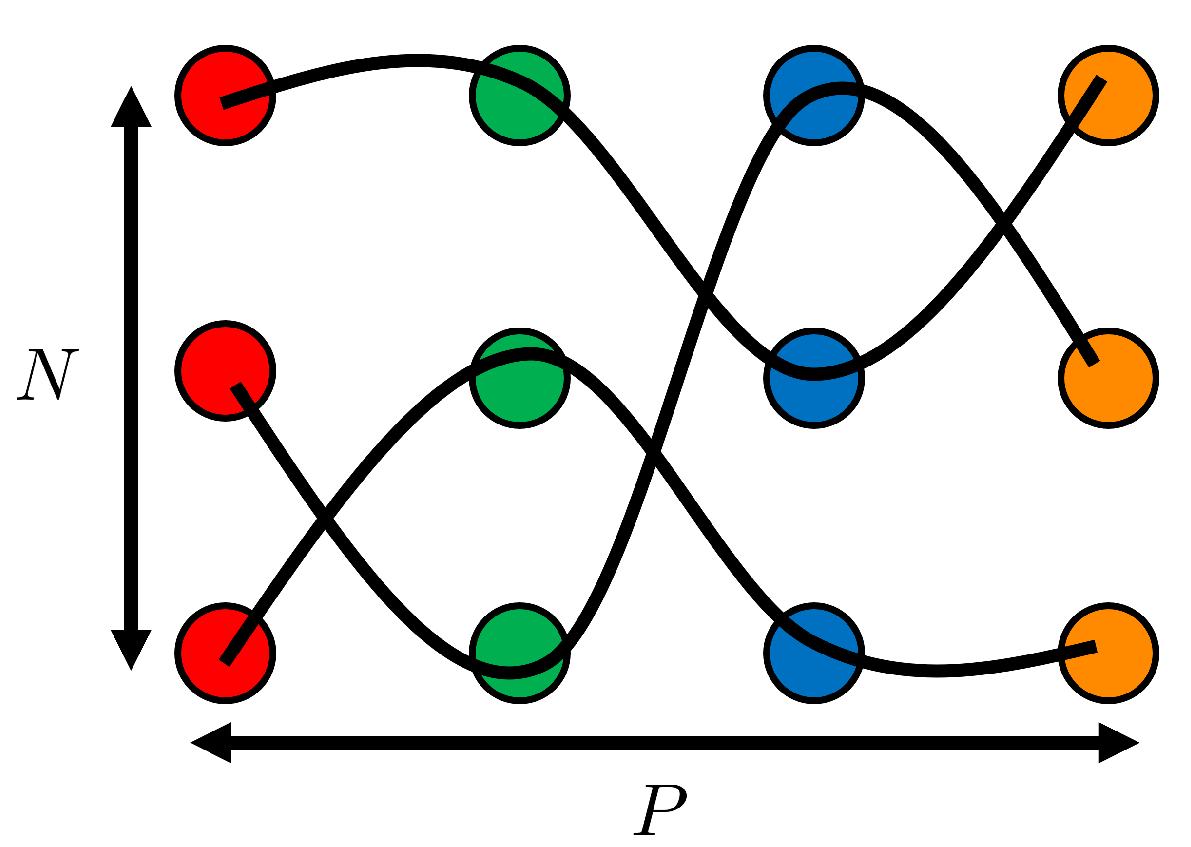
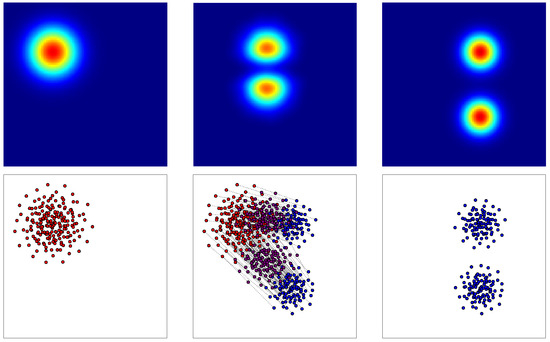 Figure 4. 1st column: Surface and its corresponding point cloud (in red). 2nd column: Partially displaced point cloud (in violet) and its corresponding reconstructed surface . The optimal matching between clouds is represented by black lines. 3rd column: Surface and its corresponding point cloud (in blue).However, the complexity of the problem significantly increases when attempting to interpolate among the surfaces sampled in . In this scenario, the optimal assignment must be performed between each surface and every other surface within the training data set. Hence, each particle of each surface should be matched with one, and only one, particle from every other surface, aiming to minimize the matching cost. The cost function is now defined among the P surfaces, summing the cost between the two surfaces for all possible pairs:This P-dimensional optimal matching involves seeking orderings , for the N particles in each surface (when matching two sets, permuting just one is sufficient, hence orderings). The P-dimensional matching problem writes:A Genetic Algorithm (GA) [35] is implemented to address this P-dimensional optimal assignment, given that this problem is equivalent to an NP-complete minimization problem. Once a reachable optimal solution is found, each particle in each surface is paired with exactly one particle from every other surface, as depicted in Figure 5. This enables us to “follow” each particle across the P surfaces.
 Figure 5. P-dimensional matching problem scheme. In this example, and . Indeed, four-point clouds of three points each can be observed. Please note that each cloud is colored differently.
 - 4.
- Regressor training: The regressor aims to learn the locations of the N particles based on the training set of P surfaces. Thus, for any point in the parametric space , it can predict the N positions of the corresponding inferred surface. To construct this parametric model, we perform a proper orthogonal decomposition (POD) [36] over the matrix of snapshots, which is composed of the x and y coordinates of the corresponding N particles reshaped as a column (reading along the rows) and this for the P decomposed training surfaces (reading along the columns).Next, we select R modes from the POD that capture sufficient information, determined by a criterion involving the relative energy of the retained snapshots. Finally, for each retained mode , a sparse Proper Generalized Decomposition (sPGD) regression [37,38] is performed on the corresponding coefficients. It can be noted that the sPGD is a robust regression technique suitable for high dimensionality without requiring a specific structure of the training data set. Indeed, when working with high-dimensional models, we must deal with the exponential growth of a basis since the growth of base elements is accompanied by the same exponential growth of data required to build the model. The sPGD technique can greatly mitigate the exponential growth of necessary data by working with a sparse training data set. This is achieved by assuming a separate representation of the solution inspired by the so-called Proper Generalized Decomposition. Moreover, the sPGD regression has a light computational training effort due to the choice of a quick-computation basis, such as a polynomial basis. The theoretical background of the sPGD is briefly presented in Appendix A.
This OT-based regression technique can be evaluated in an online manner within the parameter space of the problem. This leads to a partial displacement of all the particles, resulting in an inferred for the assessed point . Hence, the corresponding predicted surface following the optimal transport theory can be reconstructed in real time by summing all the N Gaussian functions of standard deviation at the just forecasted positions :
Finally, the total mass , which has been normalized in (13), is also inferred at to recover :
The just presented OT-based surrogate methodology is summarized in Figure 6, where the offline stage is colored in blue and the online one in red.

Figure 6.
Surrogate methodology overview: the offline stage is colored in blue and the online one in red.
5. Results
The OT-based parametric metamodeling of uncertainty propagation through the trained surrogate, as presented earlier, is now applied to the following three problems from fluid and solid dynamics:
- 1.
- a 3D steady turbulent flow into a channel facing a backward ramp.
- 2.
- a crack propagation in a notched test piece loaded in tension.
- 3.
- the design of a car dashboard aerator from the automotive manufacturer Stellantis.
For each example, we first introduce the problem and define the quantity of interest under consideration. Then, we present the problem’s surrogate g, which takes as input some parameters of the problem and returns the corresponding quantity of interest . Next, we apply the standard Monte Carlo methodology, as previously explained, to collect the mean and variance estimators of the for different values of uncertainty descriptors for the surrogate’s inputs. Finally, we train the OT-based regressors and to learn the Monte Carlo estimators for a given set of uncertainty descriptor values of the inputs, leading to the metamodel of the surrogate’s output CI.
5.1. Case 1: 3D Steady Turbulent Flow into a Channel Facing a Backward Ramp
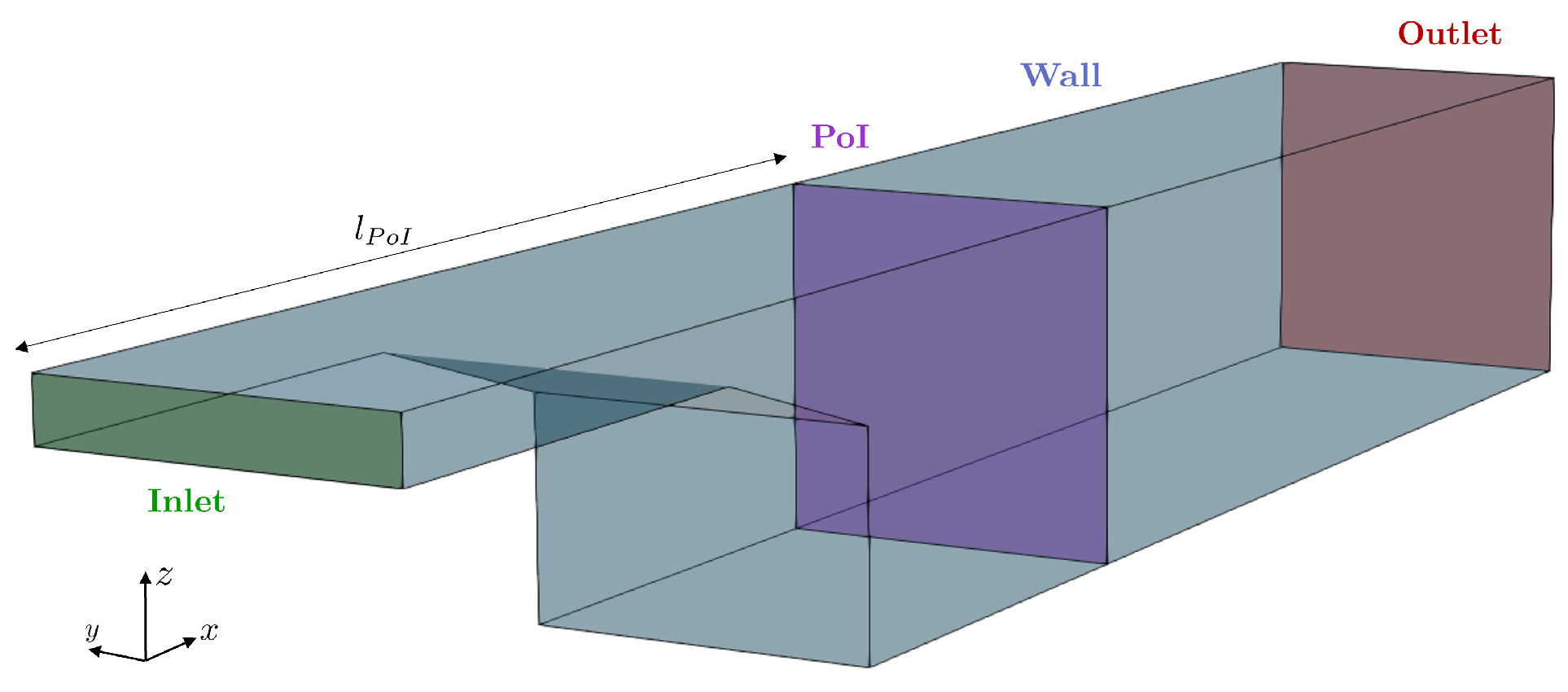
Here, we focus on a 3D steady turbulent flow into a channel facing a backward ramp, as illustrated in Figure 7. As indicated in Equation (22), the fluid, considered incompressible, exhibits a uniform velocity profile at the inlet domain with an inlet velocity of .
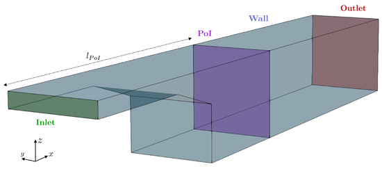
Figure 7.
Problem geometry schema.
The geometry used in this paper is close to the geometry of Ahmed’s study. The slant angle of our geometry corresponds nearly to the minimum of drag found in Ahmed’s study [39]. A nonslip condition is imposed on the walls , and a zero-gradient condition is imposed on the outlet section . Therefore, the problem is:
where is the density, the kinematic viscosity and the elementary vector of the x axis. The turbulence model chosen is SST with a stepwise switch wall function:
where is the specific dissipation rate, k the turbulent kinetic energy, y the wall-normal distance, and model constants, the kinematic viscosity of fluid near wall, the von Karman constant, the estimated wall-normal distance of the cell center in wall units and the estimated intersection of the viscous and inertial sub-layers in wall units.
The geometry is parameterized, as can be seen in Figure 8. The numerical values chosen for each parameter are collected in Table 1. It can be noted that by determining , and since is fixed, and are, thus, also fixed:

Figure 8.
Parameterized geometry.

Table 1.
Numerical values for the geometrical parameters.
Likewise, by fixing L, and , is thus also fixed by:
To solve this problem, the channel is meshed using a hexahedral mesh. The Computational Fluid Dynamics OpenFOAM code is used to solve both finite volume problems. The SIMPLE solver is chosen to solve the Navier–Stokes equations. The convergence of the simulations is ensured by monitoring the residual convergence. Moreover, the norm of the velocity field is tracked on a plane of interest perpendicular to the channel at , as represented in Figure 7.
The parameters defining the system are and , and thus . Moreover, the quantity of interest in this case is the norm of the velocity field on the plane of interest , i.e., a surface . Hence, the surrogate g takes as input the parameters and returns :
It can be noted that since the output of the system’s surrogate g is a surface, the chosen architecture for the surrogate is also the one previously introduced based on the optimal transport theory.
In this scenario, we assume that the only uncertain parameter is the kinematic viscosity . Thus, . Following the developed methodology based on the Monte Carlo estimators and optimal transport theory, we proceed to train our two regressors:
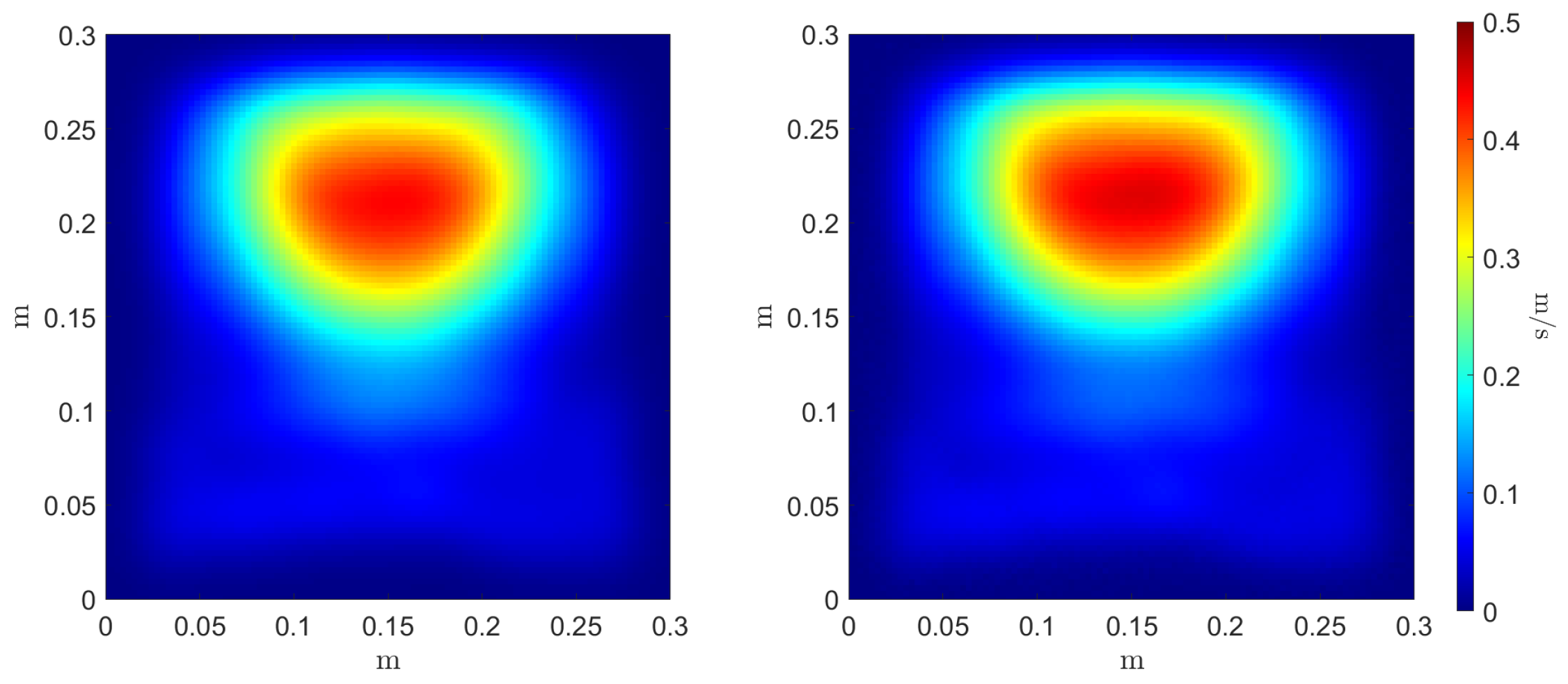
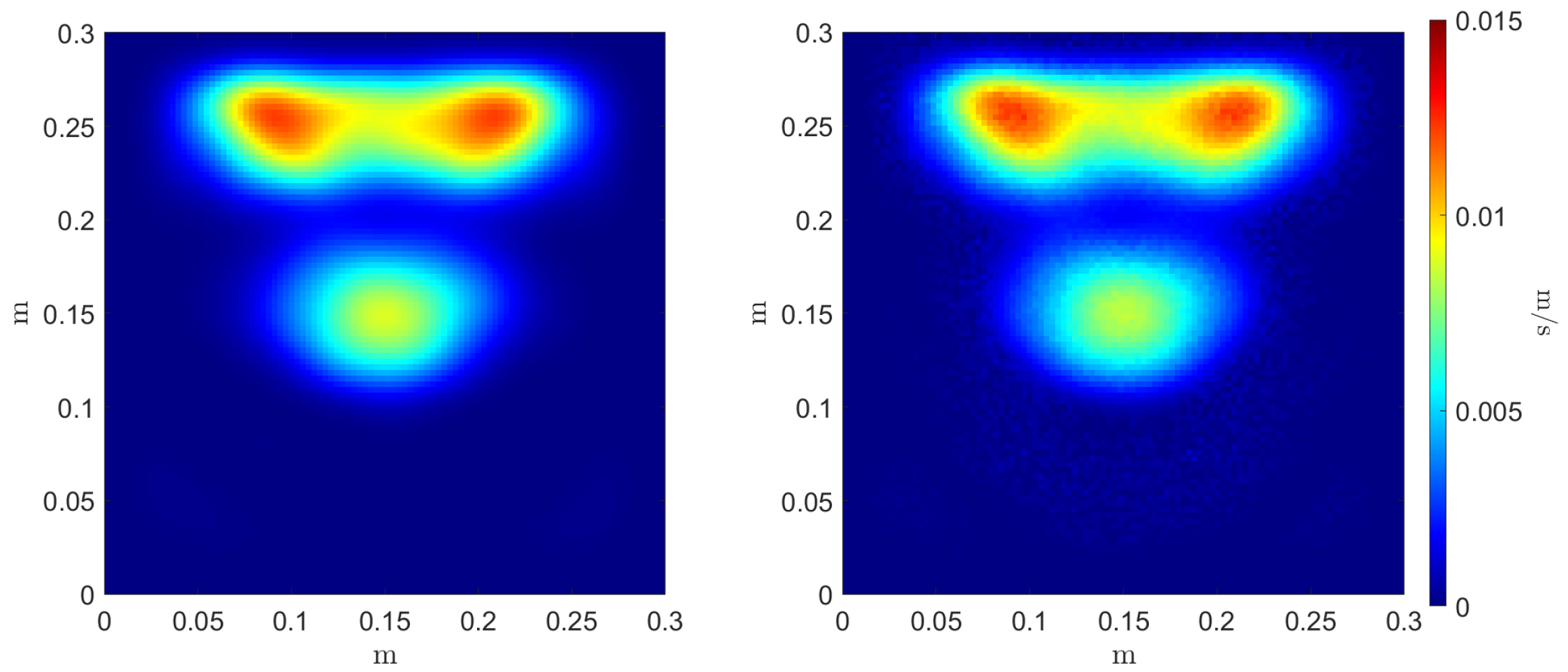
To evaluate the accuracy of the estimators’ regressors, we compare the reference and inferred Monte Carlo mean and variance estimators, as can be seen in Figure 9 and Figure 10, respectively. Three error metrics are employed over these fields concerning the maximum value magnitude and position , and the shape of the field through the 2-Wasserstein metric where the cost function c is the squared Euclidean distance. These metrics are presented in Table 2. The three errors allow a comparison between the reference estimators, denoted as f, and the inferred ones, denoted as .
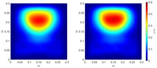
Figure 9.
Reference (left) and inferred (right) Monte Carlo mean estimator .
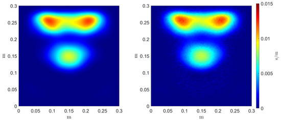
Figure 10.
Reference (left) and inferred (right) Monte Carlo variance estimator .

Table 2.
Error of the Monte Carlo estimators’ regressors.
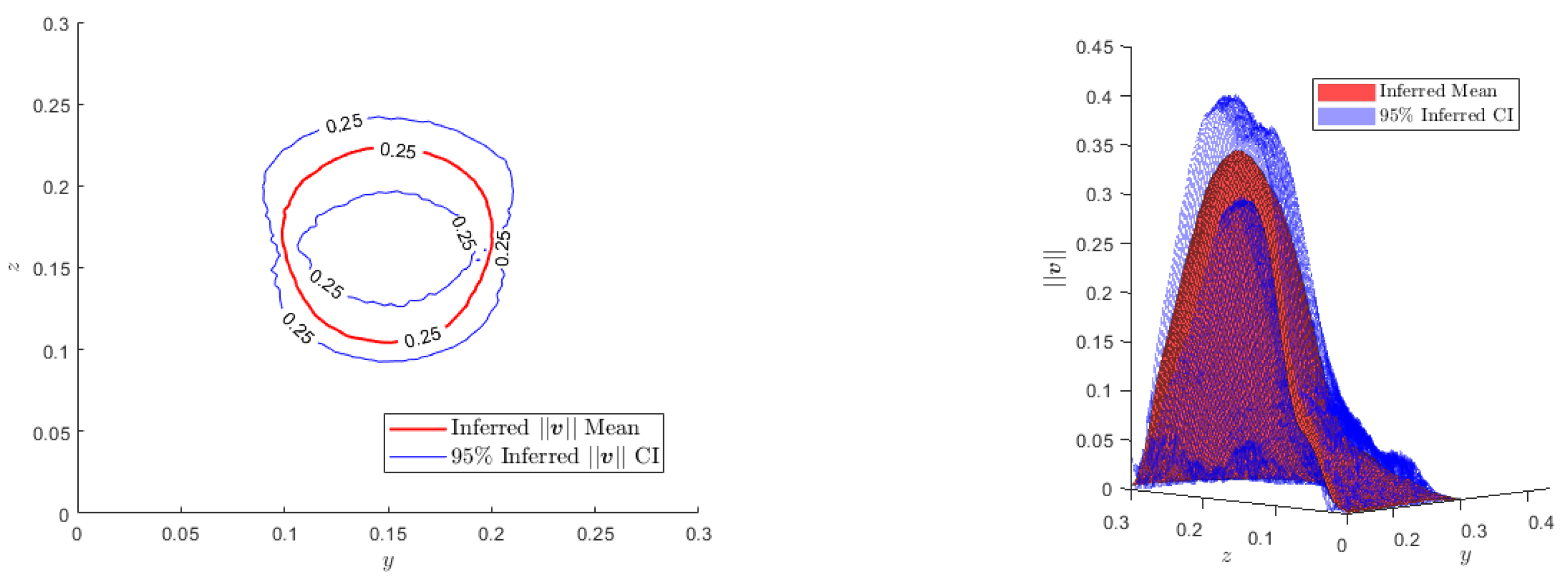
For a new test value of the uncertainty descriptors of the parameter , , we can infer the confidence interval:
where is the coefficient depending on our desired level of confidence (e.g., for a level of confidence), as can be seen in Figure 11 and Figure 12.

Figure 11.
Left: Contour plots of the inferred mean and the CI for and 0.25 m.s. Right: Inferred mean and CI for the surface of interest .
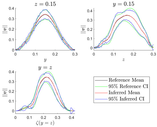
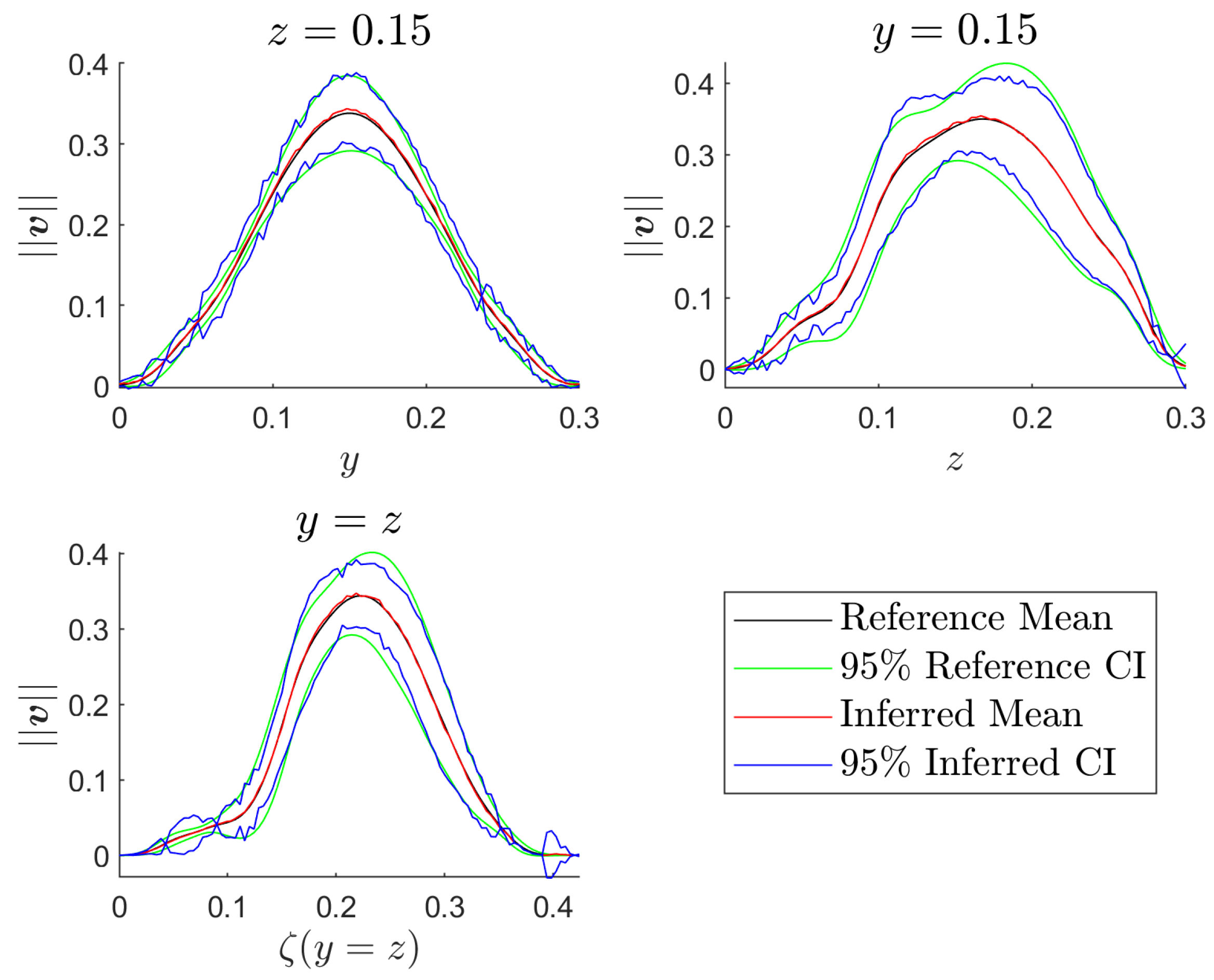
Figure 12.
Inferred and reference mean and CI for the surface of interest represented on different planes.
5.2. Case 2: Crack Propagation in a Notched Test Piece Loaded in Tension
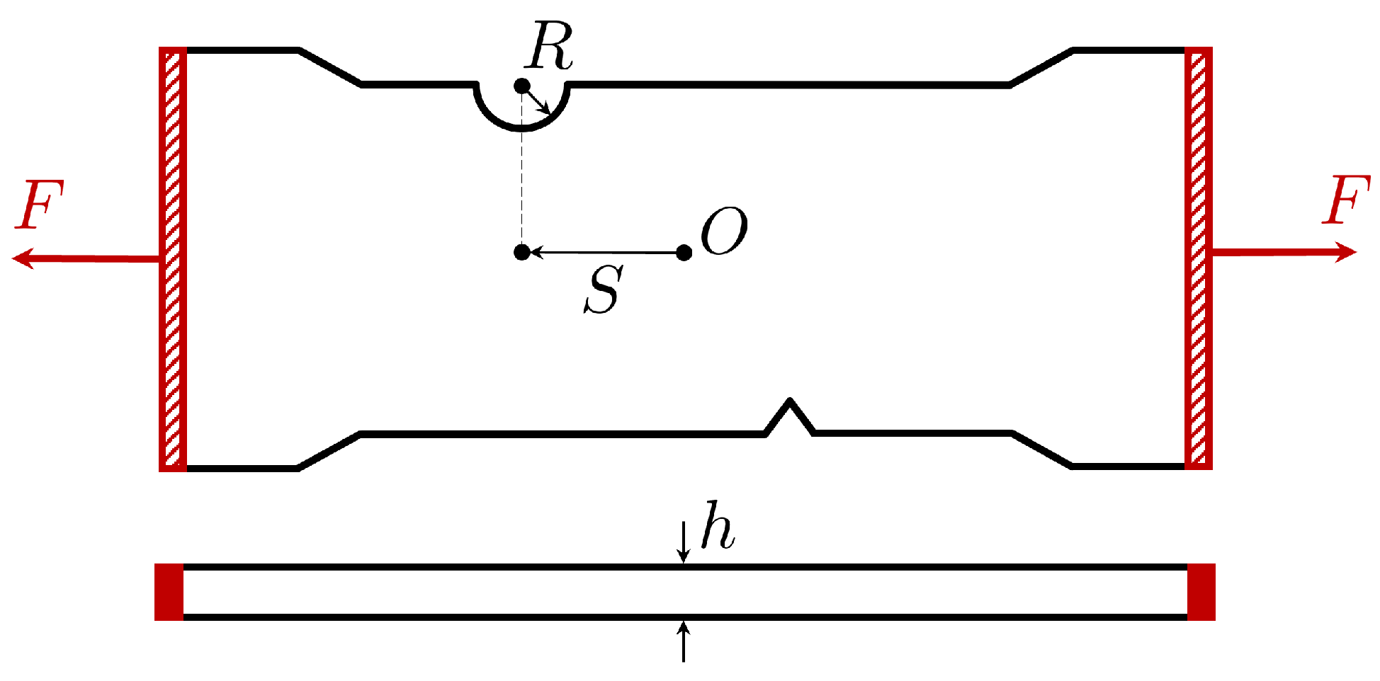
Here, we study the propagation of cracks within notched test pieces under tension loading. The geometry of the test specimens, presented in Figure 13, features a V-shaped notch defect consistently positioned near the bottom-middle region. On the opposing edge of the test piece, there exists a semi-circular groove. The objective is to forecast crack propagation from the V-shaped notch defect, considering various positions (S) and radii (R) of the groove, along with different thicknesses of the test piece (h), as schematized in Figure 13.
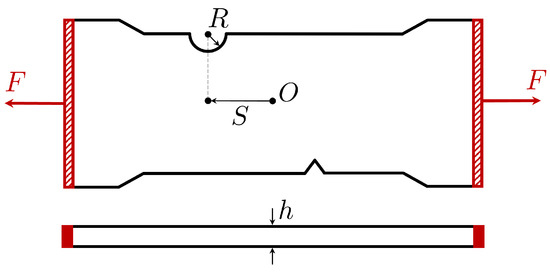
Figure 13.
Test piece scheme.
To train the surrogate of the test piece, we compute numerical simulations (carried out in the ESI Group software VPS) employing an Explicit Analysis and the EWK rupture model [40], as presented in Figure 14. It is important to note that the way the crack advances from the defect to the opposite edge of the specimen is highly dependent on the groove’s location. Two main behaviors can be observed: the crack can propagate from the defect to the groove or the opposite edge of the piece in front of the defect’s position, as illustrated in Figure 14.

Figure 14.
Main different manners of the crack propagation.
In this case, the surrogate of the problem also follows the OT-based architecture introduced before. However, a slight modification is made to the presented OT-based surrogate technique. Instead of decomposing the crack propagation field into a sum of Gaussian functions, we identify the crack and place points over it. Thus, the crack is represented by a line of N points, as can be seen in Figure 15. Then, the developed methodology can be applied to train the OT-based surrogate of the test piece, which takes the parameters R, S, and h of the piece as input and returns the 2D positions of the N points representing the crack.

Figure 15.
Left: Crack propagation field where a value of 1 represents the crack. Right: Particle representation of the crack.
The parameters defining the system are R, S, and h, and thus . In this case, the quantity of interest is the position of the crack on the test piece, represented by a 2D line , illustrated in red in Figure 15 (right), i.e., a N sets of 2-dimensional points. Hence, the surrogate g of the test piece takes as input the parameters and returns :
Here, we assume that the 3 parameters are uncertain. Hence, we suppose that , and . When computing the Monte Carlo estimators of the mean and the variance, an additional modification of the methodology should be considered.
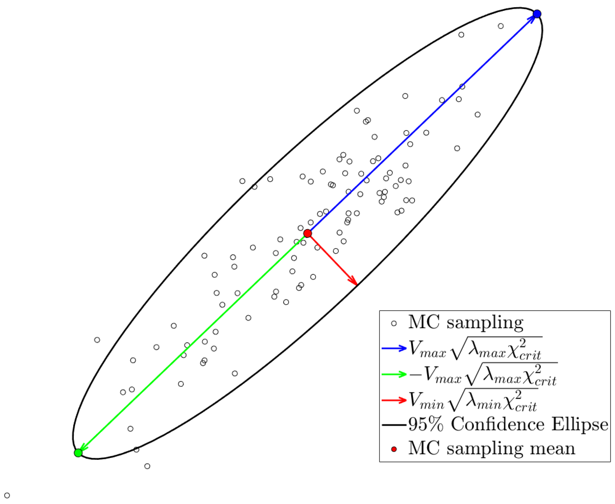
Indeed, the OT-based surrogate of the system returns the 2D positions of the N particles. Hence, for each particle, one can compute the mean of the x and y coordinates from the Monte Carlo sampling, represented by a red point in Figure 16. However, instead of computing the variance of the x and y coordinates separately, one should take into account the covariance between dimensions. To achieve this, for each particle, we compute the Confidence Ellipse. As seen in Figure 16, the sampled positions for the particle are represented for a given uncertainty descriptors of the input features. The directions of the axes of the ellipse are given by the eigenvectors of the covariance matrix. The length of the axes of the ellipse is determined by the formula:
where is the eigenvalue of the corresponding eigenvector and is the critical value of the chi-squared test . Here, degrees of freedom, and we choose a significance level of . Once computed, we keep the extremes of the major axis, represented by green and blue points in Figure 16.
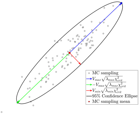
Figure 16.
sampled positions for the particle for a given uncertainty descriptors of the input features. The 95% Confidence Ellipse is plotted. and correspond to the eigenvector and eigenvalue of the largest eigenvalue, respectively. Likewise, and correspond to the eigenvector and eigenvalue of the smallest eigenvalue, respectively.
In Figure 17 (Left), the Monte Carlo sampling is illustrated for 6 particles of a crack. For each particle, the mean of the sampling and the extremes of the ellipses are identified with the same color code as in Figure 16. Once we compute the mean and the 95% Confidence Ellipses for every particle of the inferred cracks of the Monte Carlo sampling, we obtain the three estimators, , and , respectively, as presented in Figure 17 (Right).
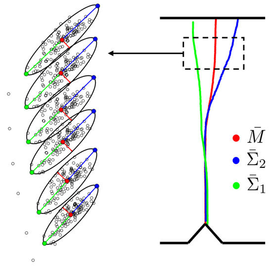
Figure 17.
Left: Monte Carlo sampling for 6 particles. The mean and the Confidence Ellipse for each particle are represented. Right: Monte Carlo estimators , and .
Then, following the developed methodology based on Monte Carlo estimators and the optimal transport theory, we train our three regressors to learn the Monte Carlo estimators of the mean crack and of the two 95% confidence limits, and .
For a new test value of the uncertainty descriptors of the parameters R, S, and h, , we can infer, as presented in Figure 18, the confidence interval:

Figure 18.
Mean crack and 95% confidence limits for two uncertainty descriptors of the input features, left and right, respectively.
In Figure 18 (left), it can be observed that, although the mean crack and one of the two 95% confidence limits follow a propagation from the defect to the groove, the other 95% confidence limit propagates to the opposite edge in front of the defect. This could be inconsistent with the two possible crack propagations defined before. However, it should be noted that the geometry shown in Figure 18 corresponds to the mean value of the Monte Carlo sampling. Indeed, it is possible that among all the sampled propagations for a given , some of the specimens’ geometries present the other possible crack propagation behavior.
5.3. Case 3: Design of a Car Dashboard Aerator
Here, we focus on the design of a car dashboard aerator from the automotive manufacturer Stellantis. The aerator is defined by 10 parameters: 8 geometrical parameters and the horizontal and vertical positions of the blades. A parametric surrogate model of the aerator is developed to study, in real time, the effect of its geometrical parameters on its performance. It can be noted that because of confidentiality issues, those geometrical parameters and the aerator geometry cannot be explicitly shown.
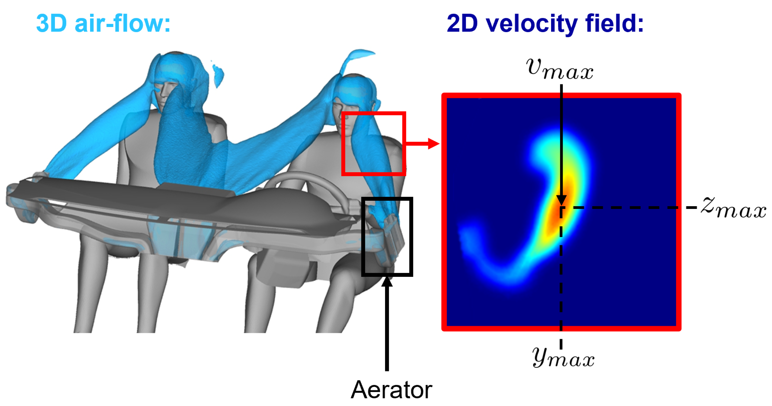
The trained aerator surrogate takes the 8 geometrical parameters of the aerator and the horizontal and vertical positions of the blades as input. It outputs the norm of the 3D velocity field of the air stream coming out from the aerator, particularized on a 2D plane representing the driver’s face, as can be seen in Figure 19. High-fidelity computational fluid dynamics simulations are computed to train the aerator surrogate.

Figure 19.
3D iso-contour of velocity for the airflow in the cockpit coming out the dashboard aerators. The plane of interest is represented in red. The amplitude of the velocity field is plotted in the plane of interest.
The performance of the aerator is quantified by assessing the position and magnitude of the maximum of this 2D scalar field. Stellantis establishes optimal values for both position and magnitude objectives based on comfort criteria. From a practical point of view, in this paper, we will focus on the left-door aerator.
The parameters defining the system are the 8 geometrical parameters of the aerator and the horizontal and vertical positions of the blades, and , respectively. Thus, . The quantity of interest is the norm of the velocity field on the plane of interest at the driver’s face, i.e., a surface . Hence, the aerator’s surrogate g takes as input the parameters and returns :
It can be noted that since the output of the aerator’s surrogate is a surface, the chosen architecture for the surrogate is the one previously introduced based on the optimal transport theory.
Here, we assume that the only uncertain parameters are the horizontal and vertical positions of the blades. The other 8 geometrical parameters of the aerator are fixed at an intermediate value. Therefore, we consider that and . Following the developed methodology based on Monte Carlo estimators and the optimal transport theory, we train our two estimators’ regressors:
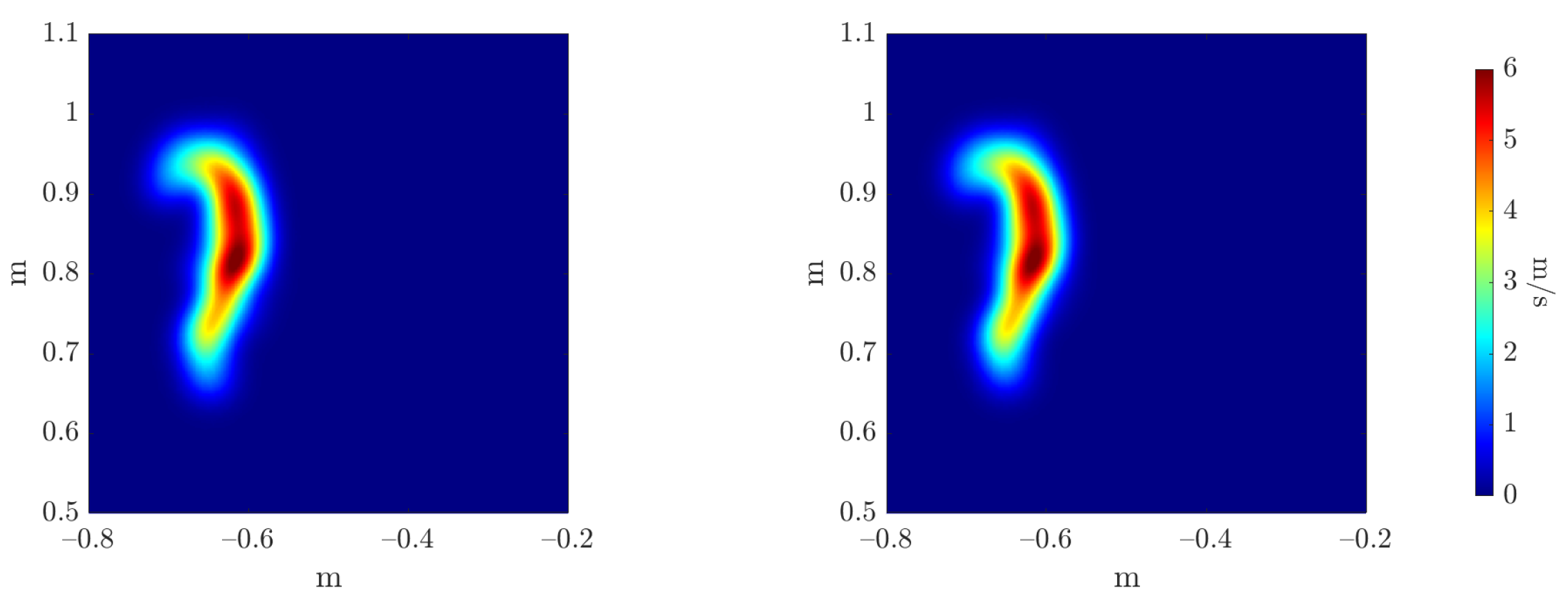
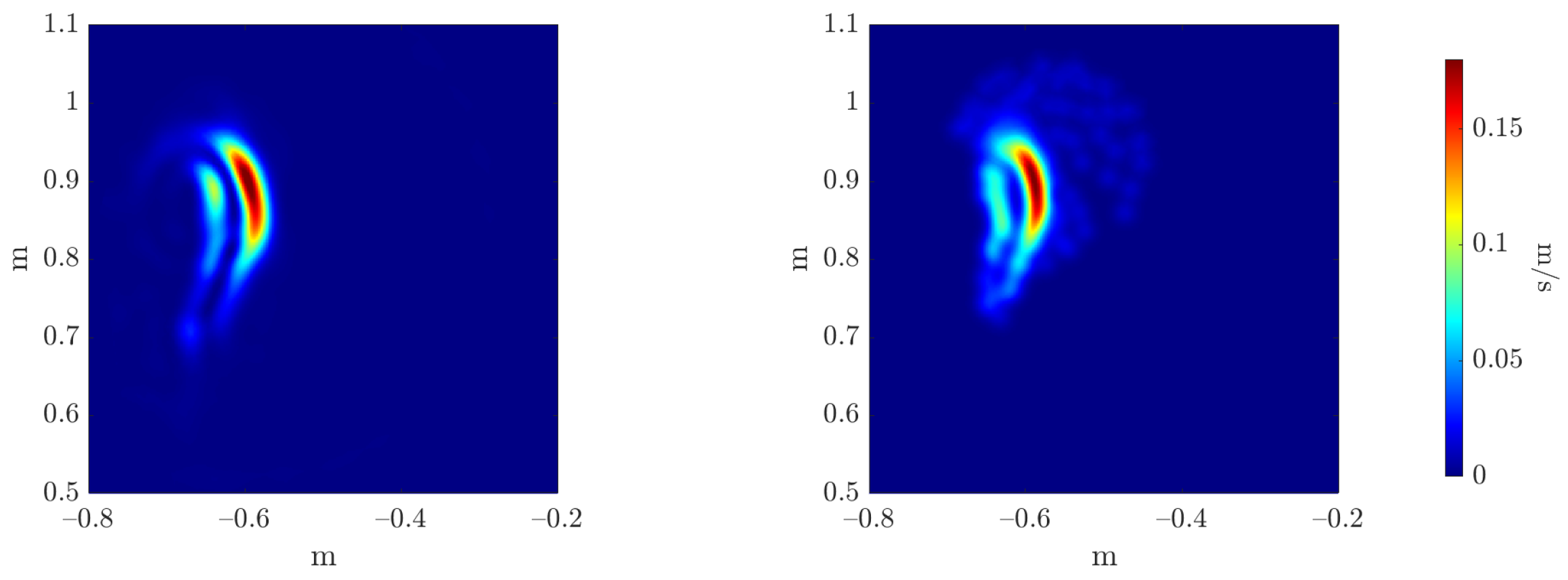
To evaluate the accuracy of the estimators’ regressors, we compare the reference and inferred Monte Carlo mean and variance estimators, as can be seen in Figure 20 and Figure 21, respectively. The three error metrics, presented in Equation (28), are applied to these fields, measuring the maximum value magnitude and position errors, and the error over the shape of the field through the 2-Wasserstein metric , as can be observed in Table 3.
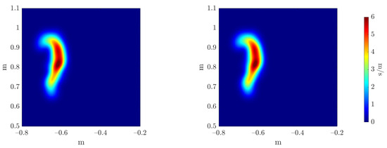
Figure 20.
Reference (left) and inferred (right) Monte Carlo mean estimator .
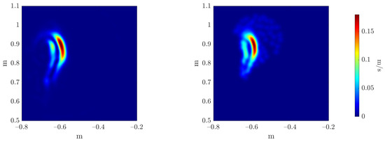
Figure 21.
Reference (left) and inferred (right) Monte Carlo variance estimator .

Table 3.
Monte Carlo estimators regressors’ errors.
For a new test value of the uncertainty descriptors of the parameters and , , we can infer the confidence interval:
where is the coefficient depending on our desired level of confidence (e.g., for a level of confidence).
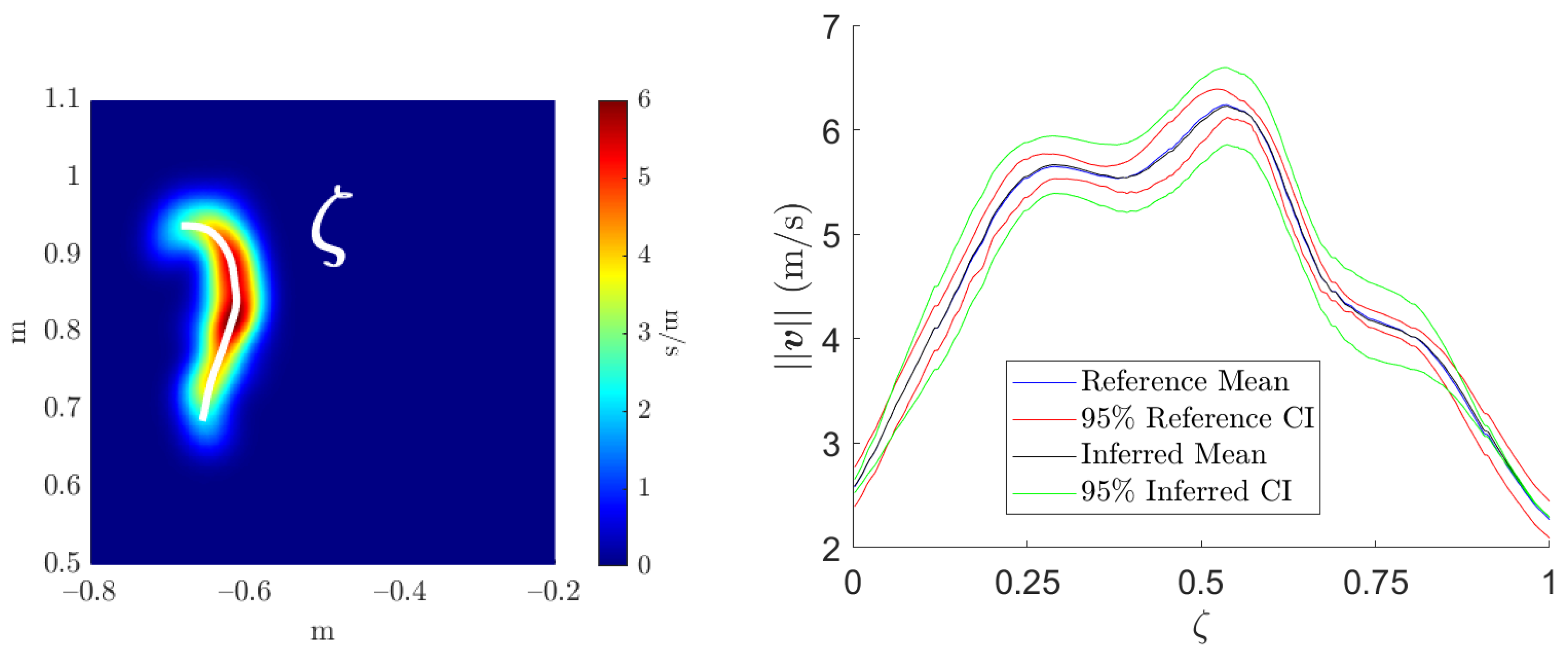
Finally, we aim to create a more practical representation of the confidence interval. Indeed, the outputs of the estimators’ surrogates are surfaces that are hardly industrially operable. Consequently, we establish a line along the maximum values of the mean estimator field, i.e., where the most information is available, as can be observed in Figure 22 (left). Then, we plot over this line the computed and inferred CI, as presented in Figure 22 (right).
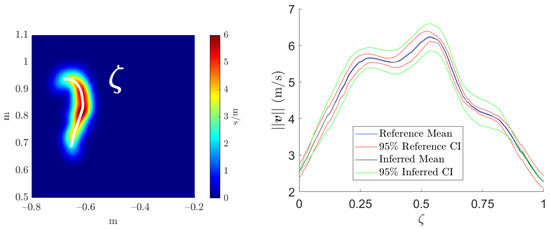
Figure 22.
Left: line over the mean estimator field. Right: computed and inferred CI.
6. Conclusions
Although data-based models of complex systems have proliferated widely, their architectures are commonly trained assuming full confidence in the knowledge of the system’s parameters, focusing exclusively on the accuracy of their outputs. In this paper, based on Monte Carlo estimators, we quantify the propagation of the uncertainty over input parameters for a given trained surrogate, focusing on its output’s precision. Then, we propose a novel regression technique based on optimal transport to infer, in real time, a confidence interval for the surrogate’s output, given a descriptor of its inputs’ uncertainty. Optimal transport provides a fundamentally distinct method for function interpolation, considered more physically relevant in various domains. However, its high computational cost becomes an issue for real-time applications. By integrating the simplified optimal transport Monge problem, equivalent to an optimal assignment problem, with the sPGD model order reduction technique, our method results in a parametric data-driven model that operates in real time, following the OT interpolation perspective.
The main drawback of this OT-based regression technique is the computational cost associated with the offline resolution of the P-dimensional matching problem, equivalent to a -complete minimization problem. Future work aims to enhance the implemented Genetic Algorithm to achieve an optimal solution or approach the P-dimensional matching problem from a different perspective, simplifying its resolution. Moreover, in ongoing research, we aim to extend this method to surrogate inputs whose uncertainty follows an unknown distribution, incorporating more sophisticated uncertainty quantification methodologies.
Author Contributions
Conceptualization, S.T., D.M., V.H. and F.C.; Methodology, S.T., D.M. and F.C.; Software, S.T. and D.M.; Validation, S.T.; Formal Analysis, S.T. and D.M.; Investigation, S.T. and D.M.; Resources, V.H. and F.C.; Data Curation, S.T. and D.M.; Writing—Original draft preparation, S.T.; Writing—Review and editing, S.T., D.M., V.H. and F.C.; Visualization, S.T.; Supervision, V.H. and F.C.; Project administration, V.H. and F.C.; Funding acquisition, V.H. and F.C.; All authors have read and agreed to the published version of the manuscript.
Funding
This research received no external funding.
Institutional Review Board Statement
The study did not require ethical approval.
Informed Consent Statement
Not applicable.
Data Availability Statement
The data presented in this study are available on request from the corresponding author. The data are not publicly available due to industrial confidentiality with STELLANTIS.
Acknowledgments
The research work was carried out at Stellantis as part of a CIFRE (Conventions Industrielles de Formation par la REcherche) thesis.
Conflicts of Interest
Authors Sergio TORREGOSA and Vincent HERBERT were employed by the company STELLANTIS. The remaining authors declare that the research was conducted in the absence of any commercial or financial relationships that could be construed as a potential conflict of interest.
Appendix A. sPGD: Sparse Proper Generalized Decomposition
Let us now consider an unknown function that we aim to approximate:
which depends on Q different variables , considered to be dimensions of the parametric space.
The sPGD tries, as standard PGD procedures, to approximate the objective function by a sum of products of one-dimensional functions. Each one of these functions represents one dimension, and each sum is known as a mode. This separated approximate expression reads:
where is the approximation, denotes the number of PGD modes and are the one-dimensional functions of the mode m and the dimension q.
In the sPGD context, the and functions are expressed from standard approximation functions:
where L is the number of degrees of freedom of the chosen approximation. Moreover, is a column vector composed of the basis functions (chosen by the user; in our case, we have chosen Chebyshev polynomials) and is a column vector that contains the coefficients for the qth dimension and the mth mode. The choice of the set of basis functions is important here and needs to suit the problem studied.
Finally, as for any other regression, the aim is to minimize the distance (here related to the L2-norm) to the measured function, finding the best approximation. This leads to the following minimization problem:
where is expressed following the separated form Equation (A2), is the number of training points, and are the vectors containing the parameters of the corresponding training point.
A greedy algorithm is employed to determine the coefficients of each one-dimensional function for each mode, such that once the approximation up to order is known, the th order is solved:
where the subscript highlights the rank of the sought function. To solve the resulting non-linear problem of the th order, an iterative scheme based on an Alternating Direction Strategy is used.
For ease of explanation and without loss of generality, let us continue by supposing that the unknown function depends on different variables: x and y. Therefore, the objective function is
which can be written in a separate form as
where and are the vectors containing the evaluation of the interpolation basis functions of the mth mode at and , respectively. Therefore, the optimization problem writes:
Then, the Alternating Direction Strategy computes from and from , where indicates the values of at the kth iteration.
Finally, the system to be solved can be written as:
where:
To conclude, the sPGD regression faces classical machine learning challenges associated with regressions: the approximation must not only fit the training set but also generalize effectively to the test set. This second objective becomes particularly difficult when dealing with sparse data in a high-dimensional problem. In this low-data limit, the risk of overfitting increases. To solve this problem, improved sPGD regressions are proposed, implementing L1 and L2 regularization techniques [38].
References
- U.S Department of Energy. Scientific Grand Challenges for National Security: The Role of Computing at the Extreme Scale. 2009. Available online: https://www.google.com.hk/url?sa=t&rct=j&q=&esrc=s&source=web&cd=&ved=2ahUKEwjridP-o_CDAxUYlK8BHS6YAX0QFnoECBUQAQ&url=https%3A%2F%2Fscience.osti.gov%2F-%2Fmedia%2Fascr%2Fpdf%2Fprogram-documents%2Fdocs%2FNnsa_grand_challenges_report.pdf&usg=AOvVaw1TmB8XWQzATNAh1bhM8K7d&opi=89978449 (accessed on 5 September 2023).
- Zhang, J. Modern Monte Carlo methods for efficient uncertainty quantification and propagation: A survey. Wiley Interdiscip. Rev. Comput. Stat. 2020, 13, e1539. [Google Scholar] [CrossRef]
- Simpson, T.W.; Poplinski, J.D.; Koch, P.N.; Allen, J.K. Metamodels for Computer-Based Engineering Design: Survey and Recommendations. Eng. Comput. 2001, 17, 129–150. [Google Scholar] [CrossRef]
- Prud’homme, C.; Rovas, D.V.; Veroy, K.; Machiels, L.; Maday, Y.; Patera, A.T. Reliable Real-Time Solution of Parametrized Partial Differential Equations: Reduced-Basis Output Bound Methods. J. Fluids Eng. 2002, 124, 70–80. [Google Scholar] [CrossRef]
- Audouze, C.; De Vuyst, F.; Nair, P.B. Nonintrusive Reduced-Order Modeling of Parametrized Time-dependent Partial Differential Equations. Numer. Methods Partial Differ. Equ. 2013, 29, 1587–1628. [Google Scholar] [CrossRef]
- Mainini, L.; Willcox, K. Surrogate Modeling Approach to Support RealTime Structural Assessment and Decision Making. AIAA 2015, 53, 1612–1626. [Google Scholar] [CrossRef]
- Hesthaven, J.S.; Rozza, G.; Stamm, B. Certified Reduced Basis Methods for Parametrized Partial Differential Equations; Springer: Berlin, Germany, 2016. [Google Scholar]
- Benner, P.; Schilders, W.; Grivet-Talocia, S.; Quarteroni, A.; Rozza, G.; Silveira, L.M. Model Order Reduction: Applications; De Gruyter: Berlin, Germany, 2020. [Google Scholar]
- Cunha, A.; Nasser, R.; Sampaio, R.; Lopes, H.; Breitman, K. Uncertainty quantification through the Monte Carlo method in a cloud computing setting. Comput. Phys. Commun. 2014, 185, 1355–1363. [Google Scholar] [CrossRef]
- Faes, M.G.; Broggi, M.; Chen, G.; Phoon, K.; Beer, M. Distribution-free P-box processes based on translation theory: Definition and simulation. Probabilistic Eng. Mech. 2022, 69, 103287. [Google Scholar] [CrossRef]
- Bi, S.; Beer, M.; Cogan, S.; Mottershead, J. Stochastic Model Updating with Uncertainty Quantification: An Overview and Tutorial. Mech. Syst. Signal Process. 2023, 204, 110784. [Google Scholar] [CrossRef]
- Faes, M.G.; Daub, S.; Marelli, E.; Patelli, E.; Beer, M. Engineering analysis with probability boxes: A review on computational methods. Struct. Saf. 2021, 93, 102092. [Google Scholar] [CrossRef]
- Wimbush, A.; Gray, N.; Ferson, S. Singhing with confidence: Visualising the performance of confidence procedures. J. Stat. Comput. Simul. 2022, 92, 2686–2702. [Google Scholar] [CrossRef]
- Lye, A.; Kitahara, M.; Broggi, M.; Patelli, E. Robust optimisation of a dynamic Black-box system under severe uncertainty: A Distribution-free framework. Mech. Syst. Signal Process. 2022, 167, 108522. [Google Scholar] [CrossRef]
- Sadeghi, J.; De Angelis, M.; Patelli, E. Efficient Training of Interval Neural Networks for Imprecise Training Data. Neural Netw. 2019, 118, 338–351. [Google Scholar] [CrossRef]
- Kalos, M.H.; Whitlock, P.A. Monte Carlo Methods; John Wiley & Sons: Hoboken, NJ, USA, 2009. [Google Scholar]
- Ghanem, R.G.; Spanos, P.D. Stochastic Finite Elements: A Spectral Approach; Courier Corporation: Chelmsford, MA, USA, 2003. [Google Scholar]
- Navarro Jimenez, M.; Le Maître, O.; Knio, O. Non-Intrusive Polynomial Chaos Expansions for Sensitivity Analysis in Stochastic Differential Equations. SIAM/ASA J. Uncertain. Quantif. 2017, 5, 278–402. [Google Scholar]
- Rasmussen, C. Gaussian Processes in Machine Learning. In Advanced Lectures on Machine Learning; Springer: Berlin/Heidelberg, Germany, 2004; pp. 63–71. [Google Scholar]
- Villani, C. Topics in Optimal Transportation; American Mathematical Soc.: Providence, RI, USA, 2003; Volume 58. [Google Scholar]
- Lévy, B.; Schwindt, E. Notions of optimal transport theory and how to implement them on a computer. Comput. Graph. 2018, 72, 135–148. [Google Scholar] [CrossRef]
- Villani, C. Optimal Transport, Old and New; Springer: Berlin/Heidelberg, Germany, 2006. [Google Scholar]
- Benamou, J.; Brenier, Y. A computational fluid mechanics solution to the Monge-Kantorovich mass transfer problem. Numer. Math. 2000, 84, 375–393. [Google Scholar] [CrossRef]
- Cuturi, M. Sinkhorn distances: Lightspeed computation of optimal transport. In Proceedings of the Advances in Neural Information Processing Systems 26: 27th Annual Conference on Neural Information Processing Systems 2013, Lake Tahoe, NV, USA, 5–8 December 2013. [Google Scholar]
- Torregrosa, S.; Champaney, V.; Ammar, A.; Herbert, V.; Chinesta, F. Surrogate Parametric Metamodel based on Optimal Transport. Math. Comput. Simul. 2021, 194, 36–63. [Google Scholar] [CrossRef]
- Wang, G.G.; Shan, S. Review of Metamodeling Techniques in Support of Engineering Design Optimization. J. Mech. Des. 2007, 129, 370–380. [Google Scholar] [CrossRef]
- Benner, P.; Gugercin, S.; Willcox, K. A Survey of Projection-Based Model Reduction Methods for Parametric Dynamical Systems. SIAM 2015, 57, 483–531. [Google Scholar] [CrossRef]
- Hesthaven, J.S.; Ubbiali, S. Non-intrusive Reduced Order Modeling of Nonlinear Problems Using Neural Networks. J. Comput. Phys. 2018, 363, 55–78. [Google Scholar] [CrossRef]
- Rajaram, D.; Perron, C.; Puranik, T.G.; Mavris, D.N. Randomized Algorithms for Non-intrusive Parametric Reduced Order Modeling. AIAA 2020, 58, 5389–5407. [Google Scholar] [CrossRef]
- Franchini, A.; Sebastian, W.; D’Ayala, D. Surrogate-based Fragility Analysis and Probabilistic Optimisation of Cable-Stayed Bridges Subject to Seismic Loads. Eng. Struct. 2022, 256, 113949. [Google Scholar] [CrossRef]
- Khatouri, H.; Benamara, T.; Breitkopf, P.; Demange, J. Metamodeling Techniques for Cpu-Intensive Simulation-Based Design Optimization: A Survey. Adv. Model. Simul. Eng. Sci. 2022, 9, 1. [Google Scholar] [CrossRef]
- Peyré, G.; Cuturi, M. Computational Optimal Transport. Found. Trends Mach. Learn. 2019, 11, 355–607. [Google Scholar] [CrossRef]
- Monge, G. Mémoire sur la Théorie des Déblais et des Remblais; Imprimerie Royale: Paris, France, 1781. [Google Scholar]
- McCann, R. A convexity principle for interacting gases. Adv. Math. 1997, 128, 153–179. [Google Scholar] [CrossRef]
- Sastry, K.; Goldberg, D.; Kendall, G. Genetic Algorithms; Springer: Boston, MA, USA, 2005; pp. 97–125. [Google Scholar]
- Chinesta, F.; Huerta, A.; Rozza, G.; Willcox, K. Encyclopedia of Computational Mechanics; John Wiley & Sons Ltd.: Hoboken, NJ, USA, 2015. [Google Scholar]
- Sancarlos, A.; Champaney, V.; Duval, J.; Cueto, E.; Chinesta, F. PGD-Based Advanced Nonlinear Multiparametric Regressions for Constructing Metamodels at the Scarce-Data Limit. Siam J. Sci. Comput. 2010. submitted. [Google Scholar]
- Pinillo, R.; Abisset-Chavanne, E.; Ammar, A.; Gonzalez, D.; Cueto, E.; Huerta, A.; Duval, J.; Chinesta, F. A multidimensional data-driven sparse identification technique: The sparse proper generalized decomposition. Complexity 2018, 2018, 5608286. [Google Scholar]
- Ahmed, S.; Ramm, G.; Faltin, G. Some Salient Features of the Time-Averaged Ground Vehicle Wake. SAE Trans. 1984, 93, 473–503. [Google Scholar]
- Kamoulakos, A. The ESI-Wilkins-Kamoulakos (EWK) Rupture Model. In Continuum Scale Simulation of Engineering Materials: Fundamentals—Microstructures—Process Applications; Wiley-VCH Verlag GmbH & Co. KGaA: Weinheim, Germany, 2005; pp. 795–804. [Google Scholar]
Disclaimer/Publisher’s Note: The statements, opinions and data contained in all publications are solely those of the individual author(s) and contributor(s) and not of MDPI and/or the editor(s). MDPI and/or the editor(s) disclaim responsibility for any injury to people or property resulting from any ideas, methods, instructions or products referred to in the content. |
© 2024 by the authors. Licensee MDPI, Basel, Switzerland. This article is an open access article distributed under the terms and conditions of the Creative Commons Attribution (CC BY) license (https://creativecommons.org/licenses/by/4.0/).

