Abstract
In response to the COVID-19 pandemic and its strain on healthcare resources, this study presents a comprehensive review of various techniques that can be used to integrate image compression techniques and statistical texture analysis to optimize the storage of Digital Imaging and Communications in Medicine (DICOM) files. In evaluating four predominant image compression algorithms, i.e., discrete cosine transform (DCT), discrete wavelet transform (DWT), the fractal compression algorithm (FCA), and the vector quantization algorithm (VQA), this study focuses on their ability to compress data while preserving essential texture features such as contrast, correlation, angular second moment (ASM), and inverse difference moment (IDM). A pivotal observation concerns the direction-independent Grey Level Co-occurrence Matrix (GLCM) in DICOM analysis, which reveals intriguing variations between two intermediate scans measured with texture characteristics. Performance-wise, the DCT, DWT, FCA, and VQA algorithms achieved minimum compression ratios (CRs) of 27.87, 37.91, 33.26, and 27.39, respectively, with maximum CRs at 34.48, 68.96, 60.60, and 38.74. This study also undertook a statistical analysis of distinct CT chest scans from COVID-19 patients, highlighting evolving texture patterns. Finally, this work underscores the potential of coupling image compression and texture feature quantification for monitoring changes related to human chest conditions, offering a promising avenue for efficient storage and diagnostic assessment of critical medical imaging.
1. Introduction
The advent of 2019 saw the emergence of a novel coronavirus, SARS-CoV-2, leading to the disease termed COVID-19. In December 2019, a rapid outbreak was noted, marking the beginning of a global health crisis [1]. The primary mode of transmission was identified to be via respiratory droplets, particularly during sneezing or coughing events from infected individuals. Furthermore, the virus demonstrated the ability to persist on surfaces, leading to potential indirect transmission [2]. The susceptibility to COVID-19 varies; elderly individuals, young children, and those with underlying medical conditions, especially respiratory ailments and diabetes, exhibit heightened vulnerability [3]. The pervasiveness of the virus can be emphasized by its presence in 213 countries and territories [4]. Notably, the highest infection rates were observed in the USA, Spain, Italy, the UK, France, Germany, China, and Canada, with the USA and Spain recording the highest mortality [5]. Governmental interventions globally have varied but predominantly focused on reducing human mobility, exemplified by the Indian government’s strategies, including lockdowns, promoting work-from-home practices, closing educational institutions, and introducing the “Aarogya Setu” contact-tracing application [6]. The mutating nature of SARS-CoV-2 has posed challenges, with noteworthy variants such as Alpha (B.1.1.7), Beta (B.1.351), Gamma (P.1), and Delta (B.1.617.2 and B.1.617.3) emerging from different regions [7]. COVID-19, also denoted as the “Novel Severe Acute Respiratory Syndrome”, primarily manifests as an infectious respiratory disease [8]. While a significant proportion of infected individuals experience mild to moderate respiratory symptoms, recovery without treatment is common. However, individuals with pre-existing conditions, including cardiovascular diseases, diabetes, chronic respiratory disorders, and cancer, tend to exhibit severe complications [9]. The critical role of vaccination in curbing the pandemic has been universally acknowledged. Several vaccines, including Pfizer-BioNTech [10], Moderna [11], Johnson & Johnson’s Janssen [12], Sputnik V [13], Covishield [14], and Covaxin [15], have been developed and administered globally [16]. The COVID-19 pandemic, caused by the SARS-CoV-2 virus, has seen multiple phases of disease transmission, often referred to as “waves”. The initial outbreak, or the “first wave”, emerged in late December 2019 and early January 2020, with a significant impact on several developed nations, including the USA, Italy, the UK, and Brazil. Remarkably, India experienced relative respite during this phase. However, the subsequent “second wave” proved devastating for India. Contributory factors included the country’s high population density and the emergence of the “Delta variant”, recognized as one of the most virulent strains of the virus. This period marked global challenges, including hospital bed shortages [17], medical oxygen scarcity [18], medical personnel deficits [19], and underreported mortality [20]. Anticipating the challenges of an expected “third wave” necessitates forward-thinking strategies, especially concerning medical data management need to be addressed. Considering the suboptimal specificity of rapid antigen-antibody tests, clinicians often advocate for chest CT scans as a more reliable diagnostic measure for COVID-19 [21]. Such a scenario underscores the potential burden on healthcare systems, given the massive data storage demands these scans entail.
Concerning the Digital Imaging and Communications in Medicine (DICOM) image compression scenario, there are two types of image compression techniques, which include lossy image compression and lossless image compression. The prominent techniques under lossy compression include transform coding [22,23], fractal compression [24,25], chroma sampling [26,27], discrete cosine transform (DCT) [28,29], and the vector quantization algorithm (VQA) [30,31]. On the other hand, lossless compression techniques include run-length encoding [32,33], entropy encoding [34,35], Lempel–Ziv–Welch (LZW) [36,37], and DEFLATE, which synergizes LZSS with Huffman coding [38,39]. Lossless compression is ideal for applications like technical drawings, and medical imaging as it preserves the quality of all original data. Conversely, lossy compression favors storage over image quality and introduces a low bit rate, resulting in significant bit rate reduction. Several research endeavors have explored a myriad of compression algorithms to address this concern. Parikh et al. [40] used high-efficiency video coding (HEVC) to compress DICOM images, achieving a commendable compression rate of over 54%. Their findings underscored the potential of the HEVC coding technique as a feasible alternative to conventional image compression methods. Rahmat et al. [41], on the other hand, championed the Huffman coding technique for lossless compression of DICOM images, with their methodology resulting in a 72.98% reduction in storage space. Ammah et al. [42] introduced a method for compressing varied medical images, including Magnetic Resonance Imaging (MRI), Computed Tomography (CT), and ultrasound images. Their approach, termed discrete wavelet transform–vector quantization (DWTVQ), was tested on multiple window sizes. Notably, they found a window size of 3 × 3 to yield optimal compression results. Sunil et al. [43] proposed an innovative medical image compression scheme utilizing the “pixel and block-level splitting technique”. Their work evaluated outcomes based on key metrics, such as the Peak Signal Noise Ratio (PSNR) and image reconstruction time, with an emphasis on lossless image compression techniques. The burgeoning realm of medical diagnostics has witnessed a significant shift towards the texture quantification approach, particularly when applied to chest CT scans. This method hinges on the mathematical quantification of image data, juxtaposing it against evolving changes in analysis [44]. A plethora of texture classification techniques burgeons in the literature, inclusive of pixel-based methods [45], feature-based methods [46], and region-based methods [47]. Delving deeper, pixel-based methods notably encapsulate techniques such as the Gray Level Co-occurrence Matrix (GLCM) [48] and the Local Binary Pattern (LBP) [49], while feature-based methods pivot around edge-based features like Scale-Invariant Feature Transform (SIFT) [50], and Speed Up Robust Features (SURF) [51]. Furthermore, region-based methods find their bifurcation into the Block Counting Method (BCM) [52] and the Active Patch Model (APM) [53]. Among these vast arrays of methodologies, the GLCM-based approach stands out in terms of its ubiquity in texture classification. Its prominence lies in its ability to simultaneously capture spectral and spatial relationships between pixels. However, the crucial question remains: what is the optimum distance and orientation angle between two pixels when deploying GLCM?
Thus, in this investigation, we propose an innovative approach, leveraging “DICOM image compression” and “texture quantification” to address data storage challenges. The system segregates DICOM images into two categories: the region of interest (ROI) and the non-region of interest (NROI). Diagnostically, the ROI holds significance, while the NROI often bears less or no diagnostic value. In our proposed method, the NROI undergoes lossy image compression, while the unaltered ROI is seamlessly incorporated into the compressed NROI. Previous advancements in DICOM image compression have laid the groundwork for this approach, as detailed in associated reviews. In the realm of medical imaging, efficient storage of DICOM images has always been paramount. The trajectory of previous research underscores the longstanding emphasis on efficient DICOM image compression. It sets a precedent for the present study, where we seek to further optimize image compression for both time and storage space conservation.
This article is systematically structured into five sections. Section 1 was about the introduction and background details of the various compression methods. Section 2 delves into the mathematical model of the proposed image compression technique and the GLCM-based texture classification features. Section 3 presents the outcomes of the conducted simulations, followed by a detailed discussion of the findings. The future scope of image compression techniques is presented in Section 4. Finally, this article concludes in Section 5, summarizing the primary insights and implications of this research.
2. Materials and Methods
2.1. Mathematical Framework for Extraction of the ROI and NROI
Identification of the ROI and image compression for DICOM images is important for the identification of diagnostically important areas from infected body parts [54]. Being digital, these images can be represented as matrices. Let us explore how digital images correspond to mathematical matrices. Essentially, every digital image is composed of pixels arranged in rows and columns, similar to the elements of a matrix. Consequently, operations applicable to matrices can similarly be performed on digital images, allowing for various mathematical manipulations and analyses.
Consider an image matrix denoted by A, represented as , where signifies the total rows and denotes the total columns of the image. Therefore, the overall pixel count within an image equals . Each pixel in the image can be pinpointed by its coordinates The pixel values for positions and within the image are bound by the constraints and The image matrix A = , can be further reconstructed using steps (1–6).
Step 1: Represent a digital image in a matrix of dimensions Thus, the image consists of a total of number of pixels.
Step 2: Extract a matrix of dimension from the input image matrix. This image matrix can be considered as the ROI. No compression or lossless compression is applied to this section of the image. Thus, the ROI matrix consists of numbers of pixels in total, which are extracted from the original image matrix.
Step 3: Apply zero padding to matrix to make the dimension of the matrix equivalent to the dimensions of matrix A matrix with zeros at a non-ROI position is called a zero-padded image matrix and is represented as Here, we have created a new matrix having all non-ROI elements zero, but the dimension of the matrix is equivalent to that of the original image matrix, i.e., .
Step 4: Perform matrix subtraction of the original image matrix with the zero-padded image matrix to obtain an image matrix with redundant information. In this step, the matrix obtained will have pixels that are of no use to us, as they represent the NROI. However, the dimensions of the matrix are the same as the original image matrix.
Step 5: Apply lossy image compression to . Thus, this region will lose its original quality and the storage required to store this will be reduced.
Step 6: Finally, fuse the lossy compressed image NROI with the non-compressed zero-padded ROI to obtain a final image with both parts embedded. This image matrix represents the final image and is expressed by .
Final image matrix
Hence, it is evident that mathematical procedures such as matrix multiplication and subtraction can be applied to digital images, including DICOM formats. These operations enable effective manipulation of both the ROI and the NROI within these images. Subsequently, these specific areas can be further processed using targeted algorithms for enhanced analysis and interpretation.
2.2. Features Derived from the
Texture classification is pivotal for discerning information regarding individual pixels in an image. The mechanism to extract both the spectral and spatial attributes from an image is facilitated by the GLCM. Haralick [55] pioneered various texture features enabling the quantification of image texture. The computation of GLCM is a two-fold process: Firstly, texture features are calculated using specified window sizes, e.g., or . Subsequently, these features undergo classification by assessing the entirety of image pixels. After GLCM’s introduction, Gotlieb et al. [56] categorized these fourteen features into four distinct clusters. If symbolizes the GLCM, and and represent the probability density functions of the image pixels, then , , , and are the respective mean and standard deviation of the image pixels for the probability density functions and . The formulations for , , , and are provided in Equations (1)–(4) [55].
is expressed as entropy , which is the entropy of the probability function.
and are expressed in Equations (5)–(8) [55].
Using Equations (1)–(8), texture features derived by the GLCM are expressed in Equations (9)–(26) [55].
Therefore, these texture features can be utilized to quantify pixel variations, facilitating the analysis of texture differences in the targeted image. This approach allows us to obtain a more detailed understanding of the image’s textural properties.
2.3. Classification of the Image Compression Algorithm
In image compression, essentially, data compression is applied to digital images which aims to minimize transmission and storage costs. Predicated on visual perception and the statistical properties of image data, these algorithms elucidate the compression process. Predominantly, image compression techniques are bifurcated into “lossless” and “lossy” categories. While both techniques minimize data redundancy, the choice between them depends on the application’s specific demands.
2.3.1. Transform Coding
Transform coding is a lossless data compression algorithm that enables digital images and audio signals to be compressed without compromising any information, thus preserving the integrity of the original data. This transformation process, while lossless, optimizes quantization to yield a “low-quality output” from the provided “input data”. The crucial part of this algorithm is the discernment of the application’s objectives. This knowledge permits non-essential areas to be pruned by “lowering the bandwidth” [57,58] while the regions of interest either remain unaltered or undergo minimal compression based on a pre-defined threshold. Consequently, while the decoded output may not be a replica of the original image, it is adequately proximate to suit the application’s needs. A schematic representation of this process, encompassing transformation, quantization, and the integration of encoding and decoding to render a reconstructed image, is depicted in Figure 1.
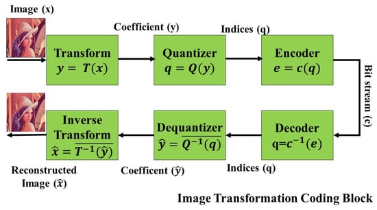
Figure 1.
Block diagram of transform coding [39].
In transform coding, the transformation block denoted as is typically invertible, ensuring that the original data can be recovered. The quantization stage, represented by introduces some distortion as it reduces the precision of the transformed data, often to compress it further [59]. However, it is important to note that the quantizer is also generally invertible, but with some loss in fidelity due to the introduced distortion. Subsequently, the encoder block, alongside the decoder, offers a lossless compression mechanism, ensuring that post-decoding, the data can be precisely reconstructed, albeit with the distortions from the quantization stage.
2.3.2. Fractal Compression
This compression technique is based on the mathematical constructs of fractals, which are self-similar patterns, where a part of the structure resembles the whole. This approach to digital image compression tends to be lossy [60,61]. The principle behind it is to find self-similar sections of an image and then use fractal mathematics to represent these sections. Visual representations of fractals can be seen in figures like the circle geometry in Figure 2a and the Sierpinski triangle in Figure 2b, both of which showcase the inherent self-similarity property of fractals.
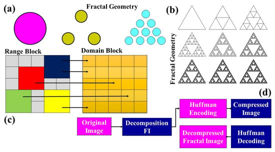
Figure 2.
Block diagram of fractal geometry and transform coding (a) Circular geometry (b) Sierpinski triangle (c) Block based compression (d) Image compression methodology [40].
Fractal compression capitalizes on the inherent redundancy found within an image. By recognizing portions of an image that are similar or identical to other sections, the method simplifies data representation. The image is partitioned into two distinct blocks: the smaller “range block” and the larger “domain block”. The technique involves using the domain block to represent or approximate the range block. For every range block, a search is conducted to find a domain block that closely mimics its appearance [62]. Figure 2c illustrates the method of fractal image compression using these blocks. To fine-tune the resemblance between domain and range blocks, a series of transformations occur encompassing shearing, rotation, scaling, translation, adjustments in brightness, contrast, and sharpness—which are applied to the domain block. The process is visualized in Figure 2d, which depicts the block diagram for image compression using fractal principles. Key characteristics of the fractal compression algorithm are:
- The achievable compression ratios range from 1:4 to 1:100, making it efficient in reducing data size.
- The compression phase is notably slower compared with other methodologies.
- Decoding, on the other hand, is expedited and is not bound by resolution constraints.
- Natural images, with their inherent similarities and patterns, are best suited for this compression method.
- The algorithm exhibits superior performance with color images as opposed to grayscale ones.
2.3.3. Chroma Sampling
Chroma subsampling is grounded in the principle of human visual perception, which is more sensitive to luminance (brightness) than to chroma (color). In this compression technique, the higher-resolution components of an image are dedicated to luminance data, while the chroma data are allocated to the lower-resolution portions [63]. Essentially, it leverages the human eye’s greater sensitivity to changes in brightness over color variations. By selectively reducing the resolution of color information and retaining more detail in brightness, chroma subsampling manages to achieve compression without a noticeable loss in perceived image quality.
The essence of chroma subsampling is predicated on the idea that humans perceive luminance information (brightness) more acutely than chromatic information (color). To exploit this characteristic of human vision, the image’s chromatic data are typically subsampled, resulting in a compressed form with less data to store or transmit while retaining a perceptual quality that is relatively indistinguishable from the original [64]. The process begins by decomposing an image’s data into two main components: luma, which represents brightness, and chroma, which carries color information. This decomposition is visually represented in Figure 3.
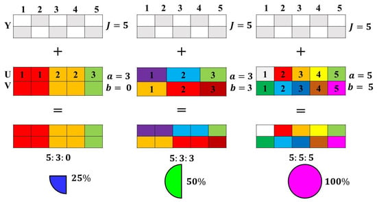
Figure 3.
Block diagram of chroma subsampling [64].
For the effective application of chroma subsampling, a transformation is essential, especially when the original image is in the RGB or CMYK model. This necessitates a shift from a model that represents colors as red, green, and blue components (or cyan, magenta, yellow, and black in CMYK) to one that distinctly demarcates brightness (luma) from color (chroma). This transformation process is typically lossless, meaning that the original image’s information remains intact and can be fully recovered. Once the image is in a suitable color space that distinctly represents luma and chroma, the subsampling can be applied predominantly to the chroma channels, leading to the desired compression.
In digital imaging, popular color spaces used for this purpose include YIQ and YCbCr. The transformation equations provided in Equations (27)–(33) detail the conversion process between these color spaces and the RGB model. These equations ensure that the transformation back and forth between the original RGB model and the chosen color space for subsampling is consistent, preserving the integrity of the original image data.
Some of the common chroma subsampling is expressed as , , , , , and The main features and subsampling methodologies are presented in Table 1.

Table 1.
Classification of the types of chroma sampling and subsampling.
2.3.4. Discrete Cosines Transform
Discrete cosine transform (DCT) has been a cornerstone in the realm of image compression for decades and forms the underpinning for JPEG, one of the most widely used image compression standards. The fundamental principle behind DCT lies in its capacity to represent an image in the frequency domain rather than its spatial domain. This property of DCT ensures that most of the image’s information is concentrated in the lower frequencies, making it particularly effective for compressing images [68,69].
One of the prominent advantages of DCT is its ability to concentrate energy within the low-frequency components of an image. This energy compaction means that most of the significant information about an image can be represented using fewer coefficients, thereby enabling effective compression. Furthermore, DCT also mitigates the “blocking artifact” phenomenon. Blocking artifacts, often visible as square block-like patterns on compressed images, are used as a common flaw in many compression algorithms. With DCT, this effect is reduced, ensuring that transitions between sub-images or blocks are more seamless and less perceptible to the human eye. These attributes, among others, make DCT an invaluable tool in various applications, from image and video processing to telecommunication systems.
After the color coordinate conversion is applied to the image, the next step is to divide the image into blocks assuming an 8 bit image. Considering the 8 bit image, the range of the element falls under The center point of this range is . So, the modified data range is shifted from to The DCT algorithm divides an image into separate parts containing different frequencies. The step-in quantization discards less critical frequencies, and the decompression stage retrieves the image with the assistance of fundamental frequencies. The 2D-DCT transformation and the inverse of the 2D-DCT transformation are expressed in Equations (34) and (35), respectively.
For and ,
When bit image, then
For and where .
2.3.5. Vector Quantization Algorithm
Linde et al. presented a vector quantization algorithm (VQA) that emerged as a pivotal lossy compression technique [70]. With its roots deeply embedded in the realms of image compression and data-hiding applications, VQA is predicated on partitioning an image into numerous distinct blocks, with each block encapsulating pixels, given as a predefined parameter. The crux of this algorithm revolves around mapping each of these blocks to a corresponding “codeword (CW)” found in a predefined “codebook”. Rather than representing the block by its actual content, the position or index of the matched CW in the codebook takes on this role in the output. During the decoding phase, the CW is systematically retrieved using its associated index values. The degree of likeness between a block and a potential CW candidate within the codebook can be gauged using a specific metric, as expressed in Equation (36). This methodology ensures efficient compression by representing large data blocks with more concise codeword indices.
where represents the entries in the state codebook, and and represent the and element corresponding to and
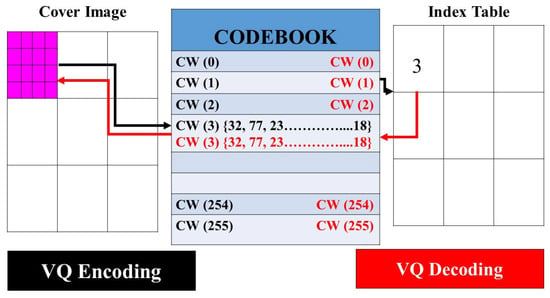
Figure 4.
Encoding–decoding procedure corresponding to the VQA [70].
Side match vector quantization (SMVQ) stands as an evolved iteration of the VQA, with its foundational premise suggesting that adjacent image pixels bear significant resemblances [71]. This enhanced variant of the algorithm, SMVQ, is acclaimed for its superior compression prowess relative to its predecessor, VQA. The modus operandi of SMVQ largely mirrors that of VQA, leveraging a VQ codebook to facilitate the coding and decoding of images. The distinguishing feature that sets SMVQ apart from VQA lies in the dimensions of the codebook; SMVQ typically uses a more compact codebook. A visualization of the pixel coding and decoding process under the VQA paradigm can be observed in Figure 4. Within this framework, individual CWs are crafted specifically for VQA encoding and decoding. The process begins with the formation of a CW, which subsequently undergoes a decoding procedure.
2.3.6. Run-Length Encoding
Run-length encoding (RLE) is a straightforward data compression technique that is particularly effective for scenarios where a dataset possesses successive instances of recurring elements. Drawing an analogy to a written “essay”, which comprises multiple paragraphs, spaces, formats, and other repetitive elements, data streams similarly exhibit repetitive patterns when transferred from one point to another [72,73]. For instance, a digital audio file may have long stretches of zeros in between songs. RLE capitalizes on these repetitive runs, compressing such stretches of redundant data to make the representation more efficient. For a clearer understanding, consider Figure 5, which visually elucidates the mechanism with which RLE compresses recurrent data sequences. Similar color represents the same data bits in the IDS and RLE schemes.

Figure 5.
Encoding model using run-length coding [74] IDS = input data stream, RLE = run-length-encoded.
RLE operates based on the principle of identifying and compressing repetitive data sequences. As illustrated in Figure 5, the encoding process kicks in whenever a data element, for example, “0” (known as the Image Data Stream or IDS), recurs. The RLE = encoded data stream then logs the element itself (“0” in this case) followed by its frequency of repetition. A critical factor for the efficacy of this algorithm is the average run length of these repetitive elements; it should exceed zero for the compression to be meaningful. RLE finds significant utility in fields like computer vision, pattern recognition, and image processing. However, it is less effective with content like natural language text where repetitive runs are either short or non-existent. Its suitability for image compression is contingent upon the image content; images with recurrent patterns or data will see notable compression, whereas those without such redundancies will not benefit much. A pivotal point to note is that it depends on the algorithm’s application and the nature of the data. The reconstructed data post-RLE compression might suffer from information loss, which might be imperceptible to human vision but can impact the data’s fidelity.
2.3.7. Entropy Encoding
Entropy encoding capitalizes on the notion that in many images, adjacent pixels are inherently related, often resulting in recurring patterns or information. This repetition, emblematic of redundancy in the data, is where entropy encoding steps in, aiming to target and compress the less correlated pixels to pare down such redundancies [75]. The process bifurcates into two phases: repetition reduction, which primarily seeks to strip away the frequencies spawned by these redundant signals, and data compression, which endeavors to excise elements of the image most immune to human visual detection. Figure 6 offers a schematic view of the entropy encoding process. It showcases two distinct blocks. The first one is the “encoder block”, which is responsible for executing the image compression, and its counterpart is the “decoder block”, which is tasked with decompressing the data to retrieve or reconstruct the original image. The mechanics of the decoder are essentially the inverse of the encoder, ensuring that the original image can be faithfully reproduced from the compressed data.
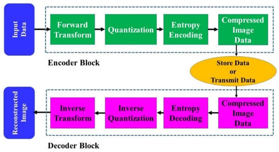
Figure 6.
Block diagram of entropy encoding [76].
Entropy encoding delves deeper into compressing signals, providing a lossless encapsulation of the original data to achieve optimal compression. The essence of this technique lies in exploiting both “spatial redundancy” and “spectral redundancy”. The former pertains to the inherent correlation that exists amongst adjacent pixels in an image. In contrast, the latter involves the correlation between distinct spectral image bands and differing color planes. Guided by these redundancies, entropy encoding calculates the likelihoods associated with each quantized value, thus creating a more efficient, probability-based code. This intelligent coding mechanism refines the output bitstream (OBS), ensuring that it is notably shorter than the input counterpart. Shannon’s entropy measure lays the foundation for this process, which is expressed by Equation (37) [75]. This mathematical expression quantifies the expected value of the information in a message or signal, serving as the bedrock for entropy-based encoding techniques.
where is an event and is the probability of the event occurring.
The data compression ratio of the “entropy of the source” and “average numbers of binary bits” is used to calculate the source data. These data represent the amount of effectiveness of the source. The significance of the compression code can be calculated as the ratio of the “entropy of the source” to the “average length of the codeword”. The source can be expressed as , where the consecutive symbol selected from is . Then the generalized probability is expressed as ,
The entropy from the source can be expanded with Equation (38).
Equation (38) can be expanded using a variable-length code and expressed by Equation (39).
The optimum code is equivalent to the entropy length and is expressed by Equation (40).
Thus, it is good to encode every with where Thus the bits are encoded in the entropy encoding.
2.3.8. Lempel–Ziv–Welch Image Compression
Lempel–Ziv–Welch (LZW) is a dictionary-based lossless compression algorithm commonly used for GIF, TIFF, and PDF formats, as shown in Figure 7. Similar color represents the similarity in the I/P and character bits. During encoding, LZW dynamically creates a dictionary of frequently recurring sequences from the input data. These sequences are then replaced with shorter dictionary codes, leading to compression. Initially, the dictionary only contains individual characters, but as more sequences are found, they are added. During decompression, the process is reversed, reconstructing the original data using the dictionary. LZW excels with repetitive data but may not significantly compress non-repetitive data [77].

Figure 7.
Coding of a general bitstream.
In LZW compression, an index table is dynamically formulated, assigning codes for strings of characters that recur in the sequence. Taking the example of the bitstream CDDCDCCCDDCCC, initial assignments are made for the characters C and D. As the bitstream progresses, sequences like DC, DCC, and CD are recognized and given new codes. Following this methodology, the 13-character sequence CDDCDCCCDDCCC is compressed to a 10-character sequence CD2C3C1D4C. Similarly, when this technique is applied to a longer 16-character bitstream CDDCDCCCDDCCCCDD, it is condensed to a 12-character sequence CD2C3C1D4C5D, as visualized in Figure 8. The similar colors represent the similarity in the I/P and character bits.

Figure 8.
Coding of a general bitstream.
The compressed bit can also be converted into the digital form per requirement. Here, it is observed that LZW performs the coding of a group of characters having variable lengths.
2.3.9. DEFLATE Image Compression
The DEFLATE algorithm, rooted in the LZ77 approach, distinguishes itself from the LZW technique. Instead of building a dynamic dictionary of data sequences, DEFLATE uses a sliding window mechanism. This window acts as a buffer, capturing chunks of data and encoding them directly. Initially, as the encoding process starts, this sliding window becomes populated with data blocks, which are then encoded. The essence of this method is its ability to identify sequential symbols, especially those with the longest match distances, and convert them into length and distance pairs. This allows the algorithm to efficiently compress files by pointing back to previous similar sequences instead of writing out each sequence afresh, leading to considerable data reduction [78,79].
The DEFLATE compression mechanism operates through a sequence of well-coordinated steps. Initially, the sliding window peruses the source file, pinpointing the “longest match” of a given block. If this match surpasses a certain threshold, the corresponding symbol is bypassed. Otherwise, the encoder determines the distance between this symbol and its longest match. This yields a (length, distance) pair, which subsequently undergoes Huffman coding to be encoded. The decoding process inverts these actions, reconstructing the original data from the (length, distance) pair based on its coded counterpart. Illustratively, Figure 9 delineates the DEFLATE operation with the LZ77 encoder at its core, outputting an LZ77-coded stream. Complementing components include a Huffman code generator and an immediate data buffer. Figure 9a lays out these modules alongside the Huffman encoder, while Figure 9b showcases preliminary data in conjunction with a symbol frequency table, detailing frequency counts for each buffered dataset.
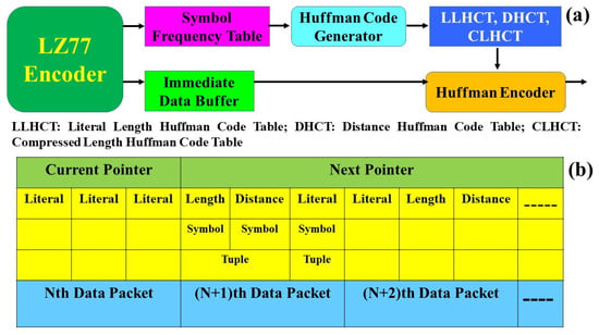
Figure 9.
The DEFLATE image compression algorithm: (a) Huffman coding and (b) a symbol frequency table.
2.4. Performance Measures for Image Compression
Several parameters can express compressed image quality. Some notable parameters through which image quality can be expressed are represented by Equations (41)–(44).
2.4.1. Mean Square Error
Mean Square Error (MSE) is a parameter with which the quality of the compressed image can be measured. The MSE between two different images and is expressed in Equation (41) [80].
where represents the input image, and is the compressed image. and represent the dimension of the input image. The MSE can be considered a relative parameter that depends entirely on the “image intensity”. Let an 8 bit image obtain an MSE value of , which means that the visual appearance of the image will not be good. At the same time, the MSE value of for a 10 bit image is hardly observable. Thus, the MSE value outcome also depends upon the bits of the image used for a study.
2.4.2. The Peak Signal to Noise Ratio
The Peak Signal to Noise Ratio (PSNR) is defined as the ratio of the input image dimension and MSE. It is measured in decibels (dB). The PSNR is considered an ideal parameter to compare the restoration result of the image. Generally, if an image has a PSNR value of it looks more exceptionally improved than an image having PSNR. The PSNR is expressed with the assistance of Equation (42) [80].
2.4.3. Compression Ratio
The compression ratio (CR) is an essential parameter with which the amount of reduced data compared with the original data is quantified. It is also known as the “compression power” and depends on the algorithm used to compress the data. It can be expressed using Equation (43) [81].
2.4.4. Bits per Pixels
Information in bits stored in a pixel of an image is known as “bits per pixel” (BPP). If an image has more numbers of bits, it can display more colors but, at the same time, also requires more space for storing the image. Increasing the memory bits of an image is necessary for displaying image quality. It can be expressed with the assistance of Equation (44) [81].
Thus, these parameters are utilized to rate the degree of compression achieved in an image compared with the original uncompressed image.
3. Results
In this section, we execute two operations on DICOM images of a CT chest infected with the COVID-19 virus. Firstly, based on matrix operations outlined in Section 2.1, we perform DICOM image processing. The DICOM images are split into ROI and NROI sections. The ROI, being diagnostically significant, can undergo lossless compression or no compression at all since it has medically important information, while the NROI is compressed using lossy compression methods. We then combine the ROI and the NROI, with which we obtain information about the superior compression technique that yields the best compression ratio. Thus, we identify the most suitable and effective image compression algorithm based on matrix-based image manipulation. Secondly, we utilize a GLCM-based approach for quantifying texture features in time-series DICOM images affected by the COVID-19 virus. This method quantifies and compares texture features across various orientations and offsets. It is an approach not previously reported in which eight offset combinations are investigated. Our unique offset combinations indicate the feasibility of texture analysis in these new directions. Ultimately, we combine both techniques to generate new insights, including the early prediction of COVID-19 infection and strategies for efficient data storage in critical situations.
3.1. ROI and NROI-Based Compression of the DICOM Image
The proposed image compression algorithm is applied to the DICOM image of the human lung infected with COVID-19 obtained from the “Center for Artificial Intelligence in Medicine & Imaging, Stanford University” [82]. DICOM is considered an international standard related to medical images. This format of medical images interchanges the data and quality necessary for medical use. , MRI, CT scans, and ultrasound are generated in the DICOM format. DICOM images have “changed the face of clinical medicine”. DICOM is approved under the “International Organization for Standardization as the standard” [83] and was developed by the “American College of Radiology ()” and “National Electrical Manufacturers Association ()” [84]. Thus, for medical image analysis, the DICOM format is considered better than other image formats. Detailed information on the DICOM image data of the patient used in this research work is presented in Table 2.

Table 2.
Detailed information on the DICOM image.
Study ID: .
Time: 11 March 2020, 11:36:03 AM.
Total DLP: .
Estimated dose saving: .
Figure 10 presents the view of the DICOM image under observation. MicroDICOM software (DICOM Viewer 2023) is used to analyze the DICOM image of the human body. The DICOM image has dimensions of . The “computed tomography (CT)” scan image used in this work shows a human lung. Since the proposed methodology is developed to be implemented on medical images, DICOM images are best suited for this application. The image compression of the DICOM is performed with the assistance of Matlab 2018 (b), with an operating system having a processor, and a hard drive.
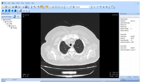
Figure 10.
representation of the human lung (MicroDICOM) [85].
The image is extracted from the software and presented in Figure 11a. The image consists primarily of two types of information, i.e., helpful information and redundant information. Valuable information is stored in the ROI, which consists of vital data about the parts of the body infected with the virus. Redundant information includes the region of the body is unaffected by the virus, which becomes unimportant from a diagnostic point of view. This redundant information is stored in the NROI region. An image under investigation can have a single or several diagnostic vital regions. These ROIs can be compressed losslessly or can be kept as is according to one’s needs. Since these are medical images, they need to be handled very carefully, and storage space reduction becomes the secondary objective while treating these images.
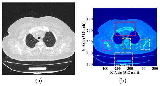
Figure 11.
(a) DICOM image of the human chest [55] (b) ROI selection from the DICOM image.
Figure 11a shows the DICOM image of the human chest with the ROI and NROI together. This image consists of too much redundant information. Let us assume that Figure 11b shows the DICOM image with four different ROIs represented by four different colors. These ROIs are considered necessary from the diagnostic point of view. These subsections are square and can be described in matrices. Thus, “lossless” or “no compression” can be applied to these regions of the DICOM image. The rest of the image is considered as the NROI, which does not have any useful information and thus can be compressed using any lossy compression technique. In this “process development”, a DICOM image with a single ROI is assumed, and the proposed methodology is implemented. A single ROI can be of any dimension, size, and shape, but the ROI used in our experiment is square.
Figure 12a represents the DICOM image with a single ROI. The ROI consists of the most vital information from a “diagnostic point of view”. The ROI can be considered an essential region consisting of information about disease. Thus, in the entire DICOM image, the ROI needs to be handled with a lot of care. This region can be compressed using “lossless compression” or “no compression”. The ROI is extracted from the DICOM image using the “sectioning technique” available in the Matlab software (R2023a). A square section of dimensions is extracted from the DICOM image, as shown in Figure 12b. It can be observed that the size of the ROI is different from the original DICOM image. Thus, any matric-based mathematical operation cannot be performed. Therefore, the zero-padding technique is applied to the ROI to create an image matrix having dimensions . In the zero-padding approach, every matrix position is filled with “zero”, leaving the ROI, and a matrix of desirable dimensions is created. This step is performed so that matrix differencing can be achieved to obtain the NROI from the DICOM image. The zero-padded image with the same dimension as the original image is presented in Figure 13a. The zero-padded image is subtracted from the original DICOM image, and the resultant image obtained after subtraction is illustrated in Figure 13b. This image does not contain any helpful information from the diagnostic point of view and is considered as the NROI. Thus, this region can be compressed using various lossy compression techniques according to one convenience and application.
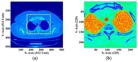
Figure 12.
(a) DICOM image of the human chest with a single ROI. (b) The extracted ROI.
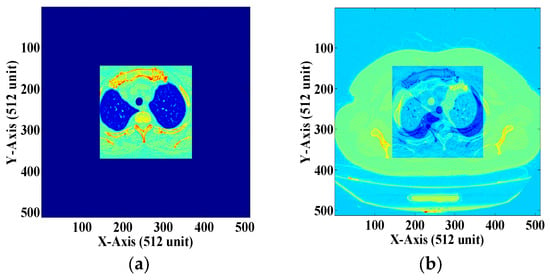
Figure 13.
(a) Zero-padded ROI image. (b) The NROI section of the DICOM image.
Here, we are aware of the medical importance of the DICOM image. Since these images are used for medical applications, we decided not to compress the ROI using any of the lossless compression schemes. The non-compressed ROI is added to the compressed NROI in its current form. However, to represent the compression effect on the ROI for education purposes, we illustrate ROI reduction in Figure 14a–d. Here, the ROI described in Figure 14a is compressed with a threshold value of 0.5. Thus, it can be observed that no or minimum loss of information occurs. Similarly, the ROI presented in Figure 14b is compressed with a threshold value of respectively, using wavelet transform. Thus, it can be visually identified that the compressed ROI has now lost information. Figure 14c shows the ROI compressed by a threshold value of . The compressed image obtained from this compression shows a drastic loss of data, which becomes dangerous for medical diagnosis. Finally, Figure 14d shows the highly compressed NROI having no input from human visual perception. Here, the threshold value is reduced to . The compression scheme used to compress the ROI is “wavelet compression”. Here, it can also be observed that with the decrease in the threshold value of compression, the visual appearance of the NROI becomes worse. It is also understood that even the ROI sections, which visually represent helpful information, may be invalid for some users. Good compression at the cost of lost data is not the objective of this research work. Thus, different lossless compression schemes can be used to compress the ROI at the same time, and no compression schemes are required to compress the ROI region.
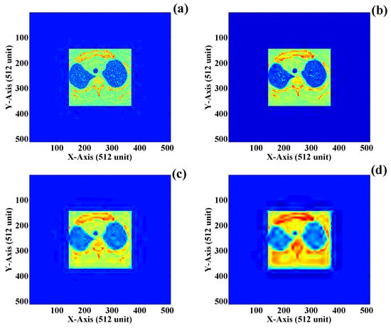
Figure 14.
Zero-padded ROI compression using wavelet transform: (a) compression factor of (b) compression factor of 0.1, (c) compression factor of and (d) compression factor of .
It is assumed that the NROI of the DICOM image does not contain any useful information that can help detect any diseases or infected parts. This image region can be compressed using “lossy image compression” techniques, which can be completed according to one perspective, i.e., one compresses the NROI part with a minimum or maximum threshold value. Since these are medical images, we advise performing lossy image compression to a desirable level so as not to affect human life. The lossy compressed NROI of the DICOM image with four different threshold values is presented in Figure 15a–d. Figure 15a presents the NROI compressed with a threshold value of Here, it can be observed that the compressed image has visually retained its essential parameters, and some critical image areas are still visually identified. Now, the threshold of compression is reduced to , and the NROI of the image begins to lose its information, as shown in Figure 15b. As the compression threshold is reduced to , the NROI part of the image loses more information, and the visual appearance of the compressed image is presented in Figure 15c. Finally, the compression threshold is reduced to , and the visual appearance of the compressed NROI is illustrated in Figure 15d. This compressed NROI does not have useful information, and the image quality is also dreadful.
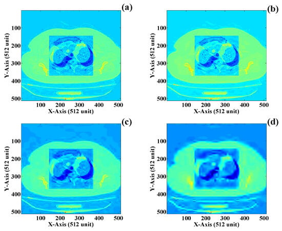
Figure 15.
NROI compression using wavelet transform: (a) compression factor of (b) compression factor of (c) compression factor of and (d) compression factor of .
Finally, the fusion of both the ROI and NROI sections of the DICOM image is completed. The fused image consists of both the compressed NROI and non-compressed ROI sections of the image. Indeed, the size of the newly compressed DICOM is less than the original DICOM. Perceptual image parameters are used to evaluate the performance parameters of the newly fused image. Different combinations of the final fused DICOM are presented in Figure 16a–d, which represent four different image thresholds having a variety of compression factors including , , and respectively. The first combination of is finalized in this work, where the ROI is added directly to the compressed NROI section. The first term of the compression factor , i.e., , indicates that no compression is applied to the ROI section of the DICOM image. The compression methodology used to compress the NROI is the lossy wavelet transform. The perceptual image quality parameters through which the effect of the image compression of the DICOM image is represented are MSE, PSNR, CR, and BPP. Table 3 presents detailed information about the perceptual image quality parameters when image compression is applied to the DICOM image using four different “lossy image compression” techniques. These compression algorithms are discrete cosine transform (DCT), discrete wavelet transform (DWT), the fractal compression algorithm (FCA), and the vector quantization algorithm (VQA), respectively. Compression time (CT*) and decompression time (DCT*) are also two factors with which the time requirement is estimated during compression and decompression of the DICOM. The CT* and DCT* indeed depend on the capacity of the workstation on which the proposed compression algorithm is performed. It may vary for different computer systems and can be less or more from the obtained results.
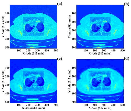
Figure 16.
Final fused image with a non-compressed ROI and a compressedNROI: (a) compression factor of (b) compression factor of (c) compression factor of and (d) compression factor of .

Table 3.
Image quality parameters for NROI sections of the DICOM image.
Figure 17a–f presents bar plots corresponding to the various perpetual image quality parameters. From Figure 17a, it can be observed that the maximum obtained MSE value corresponds to VQA and the minimum value corresponds to DCT. The lowest MSE value suggests that minimum error is generated between the original and the compressed image, which is considered suitable for image compression. Figure 17b presents the plotting for the PSNR feature. Here, it can be observed that the maximum PSNR value is obtained with the DCT algorithm, and the minimum value is obtained with the VQA. The PSNR is a prominent image quality parameter, and for efficient image compression, it should be high. Thus, since the DCT algorithm presented the highest value of the PSNR, it is regarded as an efficient image compression algorithm.
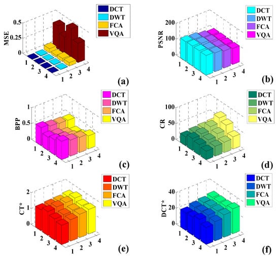
Figure 17.
Comparison of the perpetual image quality parameters: (a) MSE, (b) PSNR, (c) BPP, (d) CR, (e) CT*, and (f) DCT*.
Figure 17c compares the BPP obtained using the different image compression schemes. Here, it can be observed that BPP received the maximum value using the DCT compression algorithm and the minimum value using the VQA. Figure 17d presents a comparative plot of the CR. It can be observed that the minimum CR is obtained with the DCT algorithm, whereas the maximum compression corresponds to the VQA. The maximum CR can be symbolized as the ultimate compromise with image quality. Thus, a reasonable CR is obtained using the DCT algorithm. Figure 17e presents a comparative plot, which is minimum for the DCT algorithm and maximum for the VQA since maximum compression is obtained using the VQA. Thus, the CT* required to achieve this compression is also the largest. Finally, Figure 17f presents the DCT* of the compression algorithms. Here, the DCT algorithm obtained the minimum decompression time, whereas the VQA obtained the maximum decompression time. Thus, it is observed that the DCT algorithm emerged as an efficient and effective DICOM compression scheme. This algorithm produced good results for compressing DICOM images when compared with the other image compression algorithms. Thus, DCT can be considered best-suited for compressing DICOM images.
3.2. Texture Quantification of the Time-Series CT Chest Images
In this section, CT scans of the human chest are analyzed using a GLCM-based texture analysis approach. GLCM is a popular texture classification approach with which texture quantification of the image data is performed. GLCM offers information regarding the “spectral” and “spatial” variation in the image pixels. A time series of four CT scans of the lung chamber of a human chest infected with the COVID-19 virus is shown in Figure 18. These images are obtained from the “Italian Society of Radiology” [86]. Texture quantification of these images is performed to identify the pattern of change that developed in the visual statistical features due to the severity of the virus.

Figure 18.
Time series of CT scans of a human chest infected from COVID-19 virus (a) Day 1 (b) Day 7 (c) Day 14 (d) Day 21 [86].
Figure 18 presents the time series representation of the patient’s chest. Figure 18a illustrates the earliest image of the chest infected with the COVID-19 virus. At the same time, Figure 18b–d shows the decrease in infection in the human chest in descending order. Finally, Figure 18d illustrates the least amount of infection in the human chest. These images are converted into HSV image format to visually represent the change developed in the human chest over time. Texture quantification of the image can be performed using the GLCM technique. The GLCM calculation from an input image can be understood by reviewing Figure 19.
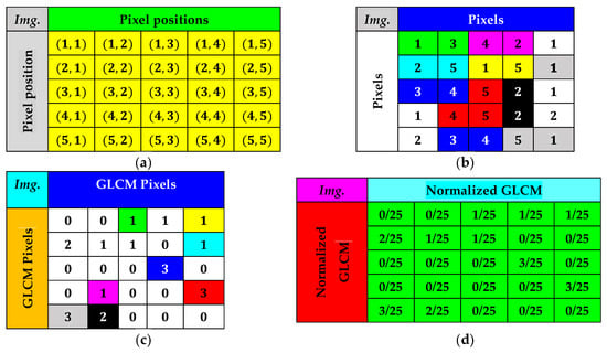
Figure 19.
Example of the GLCM calculation. (a) Pixel position in the test image of dimensions (b) Pixels in the test image. (c) GLCM obtained from the test image. (d) Normalized GLCM of the test image.
Equation (45) expresses the probability of each combination’s occurrence.
Any element in the normalized co-occurrence matrix at the position is expressed in Equation (46).
The orientation of the GLCM along different angles with a change in distance can be understood by reviewing Figure 20. Here, the orientation angles can be observed along to from the pixel of interest (POI) The distance variations can also be understood as the diagonal GLCM POI having distances , and . Similarly, several other GLCMs for an input image can be created with distances varying from to respectively.
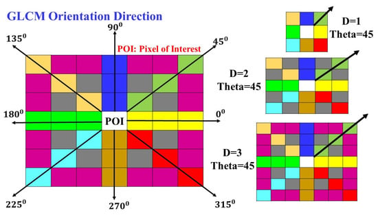
Figure 20.
GLCM with variation in the angle and distance.
Texture quantification using GLCM has two essential parameters, i.e., distance and angle. While calculating the texture feature of an image, the angle can be varied from to , , , , , and and after the following entry can be ( which is equivalent to . Similarly, is opposite to , is considered opposite to , and finally, is regarded as the opposite of . Thus, the repetitive pattern in orientation direction is obtained; therefore, only four orientation directions are considered unique in GLCM while calculating the texture features. Similarly, the distance factor varies as , , , , , , and . The offset combination of the angle and distance considering repetitive patterns for the image pixels is presented in Table 4.

Table 4.
Offset combinations for different distances and angles.
The grey-level representation of the images of the human chest infected with COVID-19 is presented in Figure 21a–d. The grey level is the false-color representation of the human chest infected with the COVID-19 virus. This image representation is presented in HSV format, which assists in identifying the changes developed in the human chest through human visual perception. As shown in Figure 21a–d, the green and yellow regions in the human chest decrease in descending order and reach a minimum in Figure 21d. The texture quantification of these images can provide information about how COVID-19 infections affect the human chest.
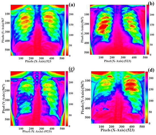
Figure 21.
Grey-level representation of the human chest infected with the COVID-19 virus in descending order of severity: (a) Day 1, (b) Day 7, (c) Day 14, and (d) Day 21.
The chest images are converted to greyscale, and later, quantification of the visual texture features is performed to obtain the change developed in the statistical image features. The numerical quantification for the different CT scans of the human chest is presented in Table 5, Table 6, Table 7 and Table 8. The quantification of the texture features provides information about the behavior of the GLCM visual texture features. The histogram signature plotting of the human chest infected with the COVID-19 virus is presented in Figure 22a–d. The histogram plots reflect the relationship between the image pixels and the intensity values. Here, it can be observed that all four images have different histogram patterns, which indicate the change developed in the CT scan of the human chest due to COVID-19.

Table 5.
Quantification of the texture features for chest CT scan corresponding to .

Table 6.
Quantification of the texture features for the chest CT scan corresponding to .

Table 7.
Quantification of the texture features for the chest condition corresponding to .

Table 8.
Quantification of the texture features for the chest condition corresponding to .
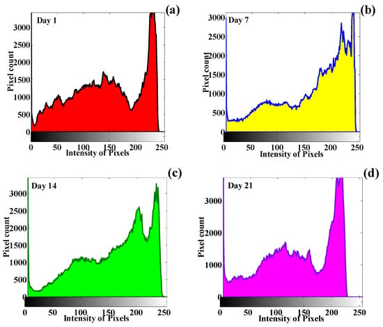
Figure 22.
Histogram signatures corresponding to time-series images of the human chest: (a) Day 1, (b) Day 7, (c) Day 14, and (d) Day 21.
The difference in the histogram pattern of the different images suggests that change occurred in the human chest’s physical structure due to the virus’s spread. This progressive change can be quantified using the GLCM technique, and changing patterns can be identified corresponding to different time-series images.
Texture classification is performed assuming four different orientations and eight different directions. Only four different exclusive orientations are considered in this research work. These unique texture features’ quantified values are included in this investigation. The quantification of the texture features for the CT scan of the human chest on is presented in Table 5. The texture plotting is performed to identify the pattern in the changing texture for different distances and orientation angles, as shown in Figure 23, Figure 24, Figure 25 and Figure 26.
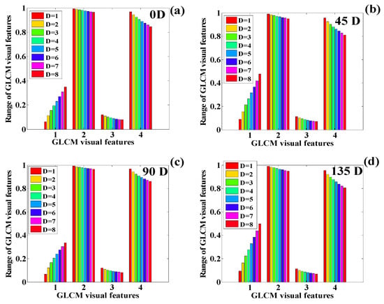
Figure 23.
Variation in the GLCM features of the human chest infected with COVID-19 (): (a) 0 degrees, (b) 45 degrees, (c) 90 degrees, (d) and 135 degrees (1 = contrast, 2 = correlation, 3 = ASM, 4 = IDM).
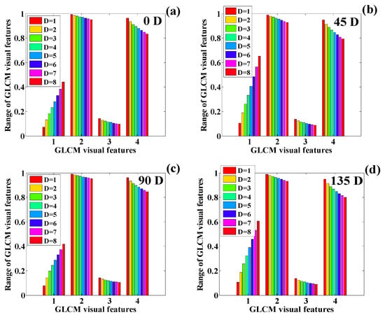
Figure 24.
Variation in the GLCM features of the human chest infected with COVID-19 (a) 0 degrees, (b) 45 degrees, (c) 90 degrees, and (d) 135 degrees (1 = contrast, 2 = correlation, 3 = ASM, 4 = IDM).
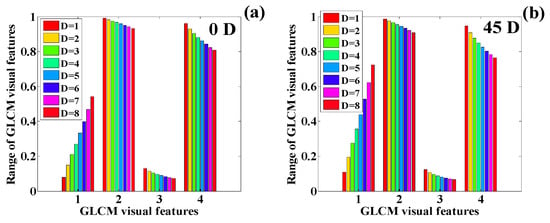
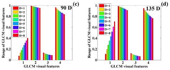
Figure 25.
Variation in the GLCM features of the human chest infected with COVID-19 (): (a) 0 degrees, (b) 45 degrees, (c) 90 degrees, and (d) 135 degrees (1 = contrast, 2 = correlation, 3 = ASM, 4 = IDM).
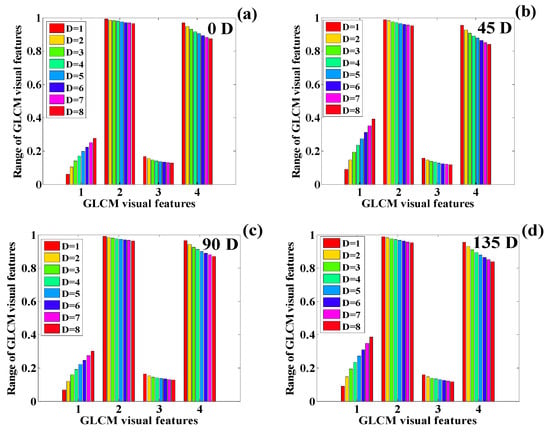
Figure 26.
Variation in the GLCM features of the human chest infected with COVID-19 (): (a) 0 degrees, (b) 45 degrees, (c) 90 degrees, and (d) 135 degrees (1 = contrast, 2 = correlation, 3 = ASM, 4 = IDM).
The variation in the GLCM visual features of the chest scan on Day 1 suggests similar behavior corresponding to the angles , , and Here, it can be observed that the contrast features increase as the distance increases, whereas correlation, ASM, and IDM decreased the feature values. By analyzing the plot thoroughly, it is observed that the contrast feature shows a rapid increase with the increase in distance. IDM demonstrates the most rapid decline rate. ASM shows a slow decline rate as compared with IDM. Finally, the decline rate correlation is almost negligible compared with ASM and IDM, respectively. Similarly, the texture quantification for the remaining three images of the human chest is performed, and their behavior is analyzed, corresponding to changes in distance and angle. Table 6 presents the quantification of texture features for
The variation in the texture features corresponding to the CT scan on is presented in Figure 24a–d. This plotting presents a similar pattern for the change in the values of the features as presented on Day 1. The contrast features show a slight increase in the texture features. IDM shows the sharpest decline in the texture features. In this case, using visual interpretation, it can be observed that correlation and ASM obtain the same pattern of reduction in the texture features.
Next, the CT scan report for is analyzed in terms of the texture features. The detailed, quantified texture features are presented in Table 7. The texture features are quantified corresponding to four orientations and eight distances.
The quantified texture features are plotted in Figure 25a–d. These feature values show the same pattern in the texture features as illustrated on and . Here, we observe a sharp rise in the texture feature contrast, whereas IDM, ASM, and correlation show a sharp decline in the texture feature values. The texture features show the same change pattern in the texture values corresponding to all four orientation directions.
Finally, the texture features of the final CT chest image are quantified to obtain the change developed in the texture features. Table 8 presents the quantified texture features.
The behavior of the texture features is presented in Figure 26a–d, which shows a similarity in the feature behavior. Here, the contrast shows the highest rise in the feature value, whereas correlation, ASM, and IDM show a decline in the feature value. It can also be observed that the feature value’s behavior is approximately similar for all four orientation angles. Finally, the average of the GLCM features obtained from the texture quantification of the CT chest images is performed, making the GLCM direction independent. The difference in the average GLCM features between two consecutive dates is performed to obtain a positive or negative change in the texture features of the images.
The differencing of the average of the GLCM features for the CT chest images 1 to 4 is performed and presented in Figure 27. This differencing is performed to observe the change developed between two consecutive CT chest images. It is observed in Figure 27 that the difference in the average texture features between I1 and I2 lies mainly on the negative side and is below zero. The contrast of the average texture features between I2 and I3 is slightly above zero and lies on the positive side. Finally, the difference between the average texture features of I3 and I4 lies mainly toward the opposing side and is below zero. Thus, several interpretations can be concluded from this study; for example, the maximum improvement in the human chest is developed between images I2 and I3 because the difference in the average texture is primarily positive. Thus, it can be concluded that using the GLCM-based texture analysis approach, the maximum amount of change developed in the CT chest scans of the human chest can be identified. The main advantage of this approach is that it provides “change information” based on the statistical arrangement of the image pixels. It is a practical methodology for change estimation. Here, GLCM application is presented for medical image processing. GLCM features are also considered unique because they can provide information on “spectral” and “spatial” arrangements. One of the shortcomings of this methodology is that it is too lengthy to implement as it contains several intermediate steps.
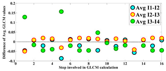
Figure 27.
Difference in the average GLCM features of the CT scans of the human chest.
4. Discussion
In this study, we conducted a comprehensive analysis of various methods used in image processing for texture quantification and image compression by examining DICOM files. CT chest scans of patients infected with the novel COVID-19 virus were utilized in this work. This investigation elegantly married two sophisticated methodologies, i.e., image compression and texture quantification, to yield insightful observations regarding the manifestations of COVID-19 infections within the human chest. Two distinct imaging techniques served as the foundational pillars of this study. DICOM imaging, which primarily underwent compression processes, and CT chest imaging, which was subject to texture quantification. The distinction between the ROI and the NROI was paramount. It was facilitated using a rigorous matrix-based mathematical algorithm. The significance of the ROI cannot be understated, given its diagnostic relevance. It encapsulates critical information about pathologies or other health anomalies. Contrarily, the NROI, while not as diagnostically critical, still plays a significant role in the overall image architecture. A suite of algorithms, namely, DCT, DWT, FCA, and VQA, were deployed to compress the NROI of the DICOM images. An intriguing observation was that the potential for heightened compression of these images certainly existed. Given their invaluable medical implications, only a calibrated level of compression was exercised. This was a strategic choice to underscore the efficiency of our proposed technique without compromising the integrity of the medical data. For empirical clarity, the achieved compression ratios ranged from 27.87 to 34.48 for DCT, from 37.91 to 68.96 for DWT, from 33.26 to 60.60 for FCA, and from 27.39 to 38.74 for VQA. Although using lossless compression on the ROI was a tangible option, our chosen methodology intentionally fused the uncompressed ROI with the compressed NROI. This approach ensured absolute data fidelity, precluding the omission of even the minutest details. Transitioning to the texture quantification of CT chest scans, we delved deep into the intricate statistical arrangements of image pixels. The use of GLCM for feature quantification painted a detailed landscape of both spatial and spectral data of the pixel configurations. The resultant quantification laid bare an intriguing pattern of texture metamorphosis over time. This not only serves as a bellwether for the progression or regression of the disease but also furnishes a multitude of diagnostic inferences. Of note was the revelation that between the time intervals I2 and I3, there was a marked positive alteration in texture features, possibly indicative of a patient’s pronounced recovery during that phase. This study further established that image processing techniques are highly efficient for data compression and storage space reduction. Each image compression technique has its advantages and disadvantages. Therefore, in our work, we endeavored to integrate various compression methods to determine the most reliable technique for image compression. A significant number of procedures were used, where the ROI was compressed using certain techniques, while the NROI was compressed utilizing others. Ultimately, we identified the most ideal combination of techniques for the analysis of DICOM images. In the current era, with the evolution of machine learning and computational intelligence techniques, several new methodologies have been introduced in image processing that can certainly produce more sound, accurate, and better results than the algorithms used in this article. Some of these notable techniques include Neural network-based image compression [87], which uses deep learning-based architectures like Convolutional Neural Networks (CNNs). These algorithms are designed to read the data for efficient image compression. Wavelet transform [88] is not a machine learning-based technique. This technique is merged with a machine learning-based algorithm for effective image compression. Evolutionary algorithms [89,90] are quite popular in image compression. One of the very popular evolutionary algorithms includes the Genetic Algorithm (GA), which can optimize image parameters for better compression, efficiency, and performance. Another popular image compression algorithm includes Fuzzy-logic systems [91], which are designed to compress an image based on its content, characteristics, and features. Generative Adversarial Networks (GANs) [92] are used to compress the image content based on high fidelity. This algorithm can create compressed images that look the same as the original image. These images cannot be distinguished from their previous vision, but the property of the compressed image is completely different from the original image. Support vector machine (SVM) [93] techniques act as a middleman, whose purpose is feature extraction and the selection of image data, based on which a suitable compression technique is selected. In the Reinforcement Learning technique [94], compression strategies are decided based on specific image characters like the compression rate and image quality. Deep reinforcement learning-based techniques [95] are considered one of the most advanced image compression techniques in which compression strategies are decided based on the type of outcome. For example, if more compression is required, then algorithms are designed in that manner, and if low compression is required, then the compression approach changes automatically. Finally, using the Convolutional Autoencoder [96] algorithm, image data can be effectively compressed by learning the spatial hierarchies of features. Currently, Artificial Intelligence (AI)-based [97,98] algorithms are in trending. These algorithms have the potential to be designed for a specific purpose and could be used for image compression purposes. In summary, this research unequivocally underscores the potency of the dual approach of image compression and texture quantification in medical image analytics. In addition to its analytical prowess, the proposed image compression algorithm could be a game-changer in data storage efficiency—a boon for the medical fraternity, especially considering the anticipated third wave of COVID-19, where rapid, efficient data processing and storage will be paramount.
5. Conclusions
This research presents a novel methodology for optimizing storage by compressing DICOM images and harnessing texture analysis to extract pivotal diagnostic information from CT chest scans. During the second wave of COVID-19, such storage efficiency became paramount. Four compression algorithms were used, including DCT, DWT, FCA, and VQA, each showing varying degrees of efficiency. The compression algorithms DCT, DWT, FCA, and VQA achieved minimum CRs of 27.87, 37.91, 33.26, and 27.39, respectively, with maximum CRs of 34.48, 68.96, 60.60, and 38.74 for the DICOM images. Finally, the texture quantification, applied to CT images of COVID-19 patients, provided insights into evolving infection patterns. Overall, our approach not only conserves storage but also enriches the diagnostic depth of medical imaging.
Author Contributions
A.K.S.: conceptualization, methodology, software, writing—original draft, investigation, and validation. A.V.: supervision and validation. All authors have read and agreed to the published version of this manuscript.
Funding
This research received no external funding.
Data Availability Statement
The datasets generated during the current study are available from the corresponding author upon reasonable request.
Acknowledgments
We express our gratitude to the developers of OpenAI’s GPT-3.5 and GPT-4.0 for their insightful and pertinent contributions.
Conflicts of Interest
The authors do not have any competing financial interests or personal relationships.
References
- Grasso, M.; Klicperová-Baker, M.; Koos, S.; Kosyakova, Y.; Petrillo, A. The impact of the coronavirus crisis on European societies. What have we learned and where do we go from here?—Introduction to the COVID volume. Eur. Soc. 2021, 23, S2–S32. [Google Scholar] [CrossRef]
- Chen, S.; Prettner, K.; Kuhn, M.; Geldsetzer, P.; Wang, C.; Bärnighausen, T.; Bloom, D.E. Climate and the spread of COVID-19. Sci. Rep. 2021, 11, 9042. [Google Scholar] [CrossRef] [PubMed]
- Varotsos, C.A.; Krapivin, V.F. A new model for the spread of COVID-19 and the improvement of safety. Saf. Sci. 2020, 132, 104962. [Google Scholar] [CrossRef]
- Xu, H.; Yan, C.; Fu, Q.; Xiao, K.; Yu, Y.; Han, D.; Wang, W.; Cheng, J. Possible environmental effects on the spread of COVID-19 in China. Sci. Total Environ. 2020, 731, 139211. [Google Scholar] [CrossRef]
- Matta, S.; Chopra, K.; Arora, V. Morbidity and mortality trends of COVID-19 in top 10 countries. Indian J. Tuberc. 2020, 67, S167–S172. [Google Scholar] [CrossRef]
- Sharma, N.; Basu, S.; Sharma, P. Sociodemographic determinants of the adoption of a contact tracing application during the COVID-19 epidemic in Delhi, India. Health Policy Technol. 2021, 10, 100496. [Google Scholar] [CrossRef]
- Chakraborty, C.; Sharma, A.R.; Bhattacharya, M.; Mallik, B.; Nandi, S.S.; Lee, S.-S. Comparative genomics, evolutionary epidemiology, and RBD-hACE2 receptor binding pattern in B.1.1.7 (Alpha) and B.1.617.2 (Delta) related to their pandemic response in UK and India. Infect. Genet. Evol. 2022, 101, 105282. [Google Scholar] [CrossRef]
- Diao, B.; Wang, C.; Wang, R.; Feng, Z.; Zhang, J.; Yang, H.; Tan, Y.; Wang, H.; Wang, C.; Liu, L.; et al. Human kidney is a target for novel severe acute respiratory syndrome coronavirus 2 infection. Nat. Commun. 2021, 12, 2506. [Google Scholar] [CrossRef]
- Gordon-Dseagu, V.L.; Shelton, N.; Mindell, J. Diabetes mellitus and mortality from all-causes, cancer, cardiovascular and respiratory disease: Evidence from the Health Survey for England and Scottish Health Survey cohorts. J. Diabetes Its Complicat. 2014, 28, 791–797. [Google Scholar] [CrossRef]
- Kudlay, D.; Svistunov, A.; Satyshev, O. COVID-19 Vaccines: An Updated Overview of Different Platforms. Bioengineering 2022, 9, 714. [Google Scholar] [CrossRef]
- Sessa, M.; Kragholm, A.H.K.; Andersen, M. Thromboembolic events in younger women exposed to Pfizer-BioNTech or Moderna COVID-19 vaccines. Expert Opin. Drug Saf. 2021, 20, 1451–1453. [Google Scholar] [CrossRef]
- Singh, A.; Khillan, R.; Mishra, Y.; Khurana, S. The safety profile of COVID-19 vaccinations in the United States. Am. J. Infect. Control 2021, 50, 15–19. [Google Scholar] [CrossRef]
- Jones, I.; Roy, P. Sputnik V COVID-19 vaccine candidate appears safe and effective. Lancet 2021, 397, 671. [Google Scholar] [CrossRef]
- Pramod, S.; Govindan, D.; Ramasubramani, P.; Kar, S.S.; Aggarwal, R. Effectiveness of Covishield vaccine in preventing COVID-19—A test-negative case-control study. Vaccine 2022, 40, 3294–3297. [Google Scholar] [CrossRef]
- Parida, S.P.; Sahu, D.P.; Singh, A.K.; Alekhya, G.; Subba, S.H.; Mishra, A.; Padhy, B.M.; Patro, B.K. Adverse events following immunization of COVID-19 (Covaxin) vaccine at a tertiary care center of India. J. Med. Virol. 2022, 94, 2453–2459. [Google Scholar] [CrossRef]
- Kudlay, D.; Svistunov, A. COVID-19 Vaccines: An Overview of Different Platforms. Bioengineering 2022, 9, 72. [Google Scholar]
- Dijkstra, S.; Baas, S.; Braaksma, A.; Boucherie, R.J. Dynamic fair balancing of COVID-19 patients over hospitals based on forecasts of bed occupancy. Omega 2022, 116, 102801. [Google Scholar] [CrossRef]
- Devereaux, A.V.; Backer, H.; Salami, A.; Wright, C.; Christensen, K.; Rice, K.; Jakel-Smith, C.; Metzner, M.; Bains, J.K.; Staats, K.; et al. Oxygen and Ventilator Logistics During California’s COVID-19 Surge: When Oxygen Becomes a Scarce Resource. Disaster Med. Public Health Prep. 2021, 17, e33. [Google Scholar] [CrossRef] [PubMed]
- Fesharaki-Zadeh, A.; Lowe, N.; Arnsten, A.F. Clinical experience with the α2A-adrenoceptor agonist, guanfacine, and N-acetylcysteine for the treatment of cognitive deficits in “Long-COVID19”. Neuroimmunol. Rep. 2023, 3, 100154. [Google Scholar] [CrossRef]
- Moeti, M.; Makubalo, L.; Gueye, A.S.; Balde, T.; Karamagi, H.; Awandare, G.; Thumbi, S.M.; Zhang, F.; Mutapi, F.; Woolhouse, M. Conflicting COVID-19 excess mortality estimates. Lancet 2023, 401, 431. [Google Scholar] [CrossRef] [PubMed]
- Attallah, O. RADIC:A tool for diagnosing COVID-19 from chest CT and X-ray scans using deep learning and quad-radiomics. Chemom. Intell. Lab. Syst. 2023, 233, 104750. [Google Scholar] [CrossRef]
- Duan, L.-Y.; Liu, J.; Yang, W.; Huang, T.; Gao, W. Video Coding for Machines: A Paradigm of Collaborative Compression and Intelligent Analytics. IEEE Trans. Image Process. 2020, 29, 8680–8695. [Google Scholar] [CrossRef]
- Ni, J.Z.F.; Noori, M.N. Deep learning for data anomaly detection and data compression of a long-span suspension bridge. Comput. Aided Civ. Infrastruct. Eng. 2020, 35, 685–700. [Google Scholar] [CrossRef]
- Liu, X.; Tong, X.; Zhang, M.; Wang, Z.; Fan, Y. Image compression and encryption algorithm based on uniform non-degeneracy chaotic system and fractal coding. Nonlinear Dyn. 2023, 111, 8771–8798. [Google Scholar] [CrossRef]
- Lu, Y.; Gong, M.; Cao, L.; Gan, Z.; Chai, X.; Li, A. Exploiting 3D fractal cube and chaos for effective multi-image compression and encryption. J. King Saud Univ. Comput. Inf. Sci. 2023, 35, 37–58. [Google Scholar] [CrossRef]
- Zou, C.; Wan, S.; Ji, T.; Blanch, M.G.; Mrak, M.; Herranz, L. Chroma Intra Prediction with Lightweight Attention-Based Neural Networks. IEEE Trans. Circuits Syst. Video Technol. 2023, 34, 549–560. [Google Scholar] [CrossRef]
- Li, X.; Du, W.; Chen, D. Object extraction from image with big size based on bilateral grid. Comput. Electr. Eng. 2023, 105, 108454. [Google Scholar] [CrossRef]
- Hong, Q.; He, B.; Zhang, Z.; Xiao, P.; Du, S.; Zhang, J. Circuit Design and Application of Discrete Cosine Transform Based on Memristor. IEEE J. Emerg. Sel. Top. Circuits Syst. 2023, 13, 502–513. [Google Scholar] [CrossRef]
- Yang, Z.-C. Data-driven discrete cosine transform (DCT)-based modeling and simulation for hourly air humidity prediction. Soft Comput. 2023, 28, 541–563. [Google Scholar] [CrossRef]
- Akhtarkavan, E.; Majidi, B.; Mandegari, A. Secure Medical Image Communication Using Fragile Data Hiding Based on Discrete Wavelet Transform and A5 Lattice Vector Quantization. IEEE Access 2023, 11, 9701–9715. [Google Scholar] [CrossRef]
- Oh, Y.; Jeon, Y.-S.; Chen, M.; Saad, W. FedVQCS: Federated Learning via Vector Quantized Compressed Sensing. IEEE Trans. Wirel. Commun. 2023. Early Access. [Google Scholar] [CrossRef]
- Kim, C.; Dao, N.-N.; Jung, K.-H.; Leng, L. Dual Reversible Data Hiding in Encrypted Halftone Images Using Matrix Encoding. Electronics 2023, 12, 3134. [Google Scholar] [CrossRef]
- Cao, W.; Leng, X.; Yu, T.; Gu, X.; Liu, Q. A Joint Encryption and Compression Algorithm for Multiband Remote Sensing Image Transmission. Sensors 2023, 23, 7600. [Google Scholar] [CrossRef]
- Viknesh, C.K.; Kumar, P.N.; Seetharaman, R.; Anitha, D. Detection and Classification of Melanoma Skin Cancer Using Image Processing Technique. Diagnostics 2023, 13, 3313. [Google Scholar] [CrossRef]
- Cui, M.; Li, K.; Li, Y.; Kamuhanda, D.; Tessone, C.J. Semi-Supervised Semantic Segmentation of Remote Sensing Images Based on Dual Cross-Entropy Consistency. Entropy 2023, 25, 681. [Google Scholar] [CrossRef] [PubMed]
- Bhatia, S.; Almutairi, A. A Robust Fuzzy Equilibrium Optimization-Based ROI Selection and DWT-Based Multi-Watermarking Model for Medical Images. Sustainability 2023, 15, 6189. [Google Scholar] [CrossRef]
- Livada, Č.; Horvat, T.; Baumgartner, A. Novel Block Sorting and Symbol Prediction Algorithm for PDE-Based Lossless Image Compression: A Comparative Study with JPEG and JPEG 2000. Appl. Sci. 2023, 13, 3152. [Google Scholar] [CrossRef]
- Sui, L.; Li, H.; Liu, J.; Xiao, Z.; Tian, A. Reversible Data Hiding in Encrypted Images Based on Hybrid Prediction and Huffman Coding. Symmetry 2023, 15, 1222. [Google Scholar] [CrossRef]
- Daoui, A.; Mao, H.; Yamni, M.; Li, Q.; Alfarraj, O.; El-Latif, A.A.A. Novel Integer Shmaliy Transform and New Multiparametric Piecewise Linear Chaotic Map for Joint Lossless Compression and Encryption of Medical Images in IoMTs. Mathematics 2023, 11, 3619. [Google Scholar] [CrossRef]
- Parikh, S.S.; Ruiz, D.; Kalva, H.; Fernández-Escribano, G.; Adzic, V. High Bit-Depth Medical Image Compression with HEVC. IEEE J. Biomed. Health Inform. 2018, 22, 552–560. [Google Scholar] [CrossRef]
- Rahmat, R.F.; Andreas, T.S.M.; Fahmi, F.; Pasha, M.F.; Alzahrani, M.Y.; Budiarto, R. Analysis of DICOM Image Compression Alternative Using Huffman Coding. J. Healthc. Eng. 2019, 2019, 5810540. [Google Scholar] [CrossRef]
- Ammah, P.N.T.; Owusu, E. Robust medical image compression based on wavelet transform and vector quantization. Inform. Med. Unlocked 2019, 15, 100183. [Google Scholar] [CrossRef]
- Sunil, H.; Hiremath, S.G. A combined scheme of pixel and block level splitting for medical image compression and reconstruction. Alex. Eng. J. 2018, 57, 767–772. [Google Scholar] [CrossRef]
- Voigt, M.; Miller, J.A.; Mainza, A.N.; Bam, L.C.; Becker, M. The Robustness of the Gray Level Co-Occurrence Matrices and X-Ray Computed Tomography Method for the Quantification of 3D Mineral Texture. Minerals 2020, 10, 334. [Google Scholar] [CrossRef]
- Yan, Z.; Ma, L.; He, W.; Zhou, L.; Lu, H.; Liu, G.; Huang, G. Comparing Object-Based and Pixel-Based Methods for Local Climate Zones Mapping with Multi-Source Data. Remote Sens. 2022, 14, 3744. [Google Scholar] [CrossRef]
- Humeau-Heurtie, A. Texture Feature Extraction Methods: A Survey. IEEE Access 2019, 7, 8975–9000. [Google Scholar] [CrossRef]
- Alpaslan, N.; Hanbay, K. Multi-Resolution Intrinsic Texture Geometry-Based Local Binary Pattern for Texture Classification. IEEE Access 2020, 8, 54415–54430. [Google Scholar] [CrossRef]
- Ramola, A.; Shakya, A.K.; Van Pham, D. Study of statistical methods for texture analysis and their modern evolutions. Eng. Rep. 2020, 2, e12149. [Google Scholar] [CrossRef]
- Kaplan, K.; Kaya, Y.; Kuncan, M.; Ertunç, H.M. Brain tumor classification using modified local binary patterns (LBP) feature extraction methods. Med. Hypotheses 2020, 139, 109696. [Google Scholar] [CrossRef]
- Chen, S.; Zhong, S.; Xue, B.; Li, X.; Zhao, L.; Chang, C.-I. Iterative Scale-Invariant Feature Transform for Remote Sensing Image Registration. IEEE Trans. Geosci. Remote. Sens. 2020, 59, 3244–3265. [Google Scholar] [CrossRef]
- Gupta, S.; Thakur, K.; Kumar, M. 2D-human face recognition using SIFT and SURF descriptors of face’s feature regions. Vis. Comput. 2020, 37, 447–456. [Google Scholar] [CrossRef]
- Nayak, S.R.; Mishra, J.; Palai, G. Analysing roughness of surface through fractal dimension: A review. Image Vis. Comput. 2019, 89, 21–34. [Google Scholar] [CrossRef]
- Gozum, M.M.; Serhat, G.; Basdogan, I. A semi-analytical model for dynamic analysis of non-uniform plates. Appl. Math. Model. 2019, 76, 883–899. [Google Scholar] [CrossRef]
- Shakya, A.K.; Ramola, A.; Pandey, D.C. Polygonal region of interest-based compression of DICOM images. In Proceedings of the International Conference on Computing Communication and Automation (ICCCA), Noida, India, 5–6 May 2017. [Google Scholar]
- Haralick, R.M.; Shanmugam, K.; Dinstein, I. Textural Features for Image Classification. IEEE Trans. Syst. Man Cybern. 1973, SMC-3, 610–621. [Google Scholar] [CrossRef]
- Gotlieb, C.C.; Kreyszig, H.E. Texture descriptors based on co-occurrence matrices. Comput. Vis. Graph. Image Process. 1990, 51, 70–86. [Google Scholar] [CrossRef]
- Zhao, J.; Wang, S.; Zhang, L. Block Image Encryption Algorithm Based on Novel Chaos and DNA Encoding. Information 2023, 14, 150. [Google Scholar] [CrossRef]
- Wang, J.; Tan, F.S.; Yuan, Y. Random Matrix Transformation and Its Application in Image Hiding. Sensors 2023, 23, 1017. [Google Scholar] [CrossRef]
- Starosolski, R. Hybrid Adaptive Lossless Image Compression Based on Discrete Wavelet Transform. Entropy 2020, 22, 751. [Google Scholar] [CrossRef]
- Petráš, I. Novel Low-Pass Two-Dimensional Mittag–Leffler Filter and Its Application in Image Processing. Fractal Fract. 2023, 7, 881. [Google Scholar] [CrossRef]
- Aldakheel, E.A.; Khafaga, D.S.; Fathi, I.S.; Hosny, K.M.; Hassan, G. Efficient Analysis of Large-Size Bio-Signals Based on Orthogonal Generalized Laguerre Moments of Fractional Orders and Schwarz–Rutishauser Algorithm. Fractal Fract. 2023, 7, 826. [Google Scholar] [CrossRef]
- Kumar, R.S.; Manimegalai, P. Near lossless image compression using parallel fractal texture identification. Biomed. Signal Process. Control. 2020, 58, 101862. [Google Scholar] [CrossRef]
- Wiseman, Y. Adapting the H.264 Standard to the Internet of Vehicles. Technologies 2023, 11, 103. [Google Scholar] [CrossRef]
- Babu, C.; Chandy, D.A.; Karthigaikumar, P. Novel chroma subsampling patterns for wireless capsule endoscopy compression. Neural Comput. Appl. 2019, 32, 6353–6362. [Google Scholar] [CrossRef]
- Heindel, A.; Prestele, B.; Gehlert, A.; Kaup, A. Enhancement Layer Coding for Chroma Sub-Sampled Screen Content Video. IEEE Trans. Circuits Syst. Video Technol. 2021, 32, 788–801. [Google Scholar] [CrossRef]
- Lin, T.-L.; Liu, B.-H.; Jiang, K.-H. An Efficient Algorithm for Luminance Optimization in Chroma Downsampling. IEEE Trans. Circuits Syst. Video Technol. 2020, 31, 3719–3724. [Google Scholar] [CrossRef]
- Baracchi, D.; Shullani, D.; Iuliani, M.; Giani, D.; Piva, A. Camera Obscura: Exploiting in-camera processing for image counter forensics. Forensic Sci. Int. Digit. Investig. 2021, 38, 301213. [Google Scholar] [CrossRef]
- Zhu, Y.; Fan, L.; Li, Q.; Chang, J. Multi-Scale Discrete Cosine Transform Network for Building Change Detection in Very-High-Resolution Remote Sensing Images. Remote Sens. 2023, 15, 5243. [Google Scholar] [CrossRef]
- Liu, H.; Zhang, X.; Dong, H.; Liu, Z.; Hu, X. Magnetic Anomaly Detection Based on Energy-Concentrated Discrete Cosine Wavelet Transform. IEEE Trans. Instrum. Meas. 2023, 72, 9700210. [Google Scholar] [CrossRef]
- Linde, Y.; Buzo, A.; Gray, R. An Algorithm for Vector Quantizer Design. IEEE Trans. Commun. 1980, 28, 84–95. [Google Scholar] [CrossRef]
- Fadel, M.M.; Said, W.; Hagras, E.A.A.; Arnous, R. A Fast and Low Distortion Image Steganography Framework Based on Nature-Inspired Optimizers. IEEE Access 2023, 11, 125768–125789. [Google Scholar] [CrossRef]
- Soni, E.; Nagpal, A.; Garg, P.; Pinheiro, P.R. Assessment of Compressed and Decompressed ECG Databases for Telecardiology Applying a Convolution Neural Network. Electronics 2022, 11, 2708. [Google Scholar] [CrossRef]
- Chianphatthanakit, C.; Boonsongsrikul, A.; Suppharangsan, S. Differential Run-Length Encryption in Sensor Networks. Sensors 2019, 19, 3190. [Google Scholar] [CrossRef]
- Dai, B.; Yin, S.; Gao, Z.; Wang, K.; Zhang, D.; Zhuang, S.; Wang, X. Data Compression for Time-Stretch Imaging Based on Differential Detection and Run-Length Encoding. J. Light. Technol. 2017, 35, 5098–5104. [Google Scholar] [CrossRef]
- Ahmed, K.; Nadeem, M.I.; Li, D.; Zheng, Z.; Ghadi, Y.Y.; Assam, M.; Mohamed, H.G. Exploiting Stacked Autoencoders for Improved Sentiment Analysis. Appl. Sci. 2022, 12, 12380. [Google Scholar] [CrossRef]
- Kumar, B.S.; Manjunath, A.; Christopher, S. Improved entropy encoding for high efficient video coding standard. Alex. Eng. J. 2018, 57, 1–9. [Google Scholar] [CrossRef]
- Rahman, M.A.; Hamada, M. Lossless Image Compression Techniques: A State-of-the-Art Survey. Symmetry 2019, 11, 1274. [Google Scholar] [CrossRef]
- Hwang, G.B.; Cho, K.N.; Han, C.Y.; Oh, H.W.; Yoon, Y.H.; Lee, S.E. Lossless Decompression Accelerator for Embedded Processor with GUI. Micromachines 2021, 12, 145. [Google Scholar] [CrossRef]
- Tu, K.; Puchala, D. Variable-to-Variable Huffman Coding: Optimal and Greedy Approaches. Entropy 2022, 24, 1447. [Google Scholar] [CrossRef]
- Shubham, S.; Bhandari, A.K. A generalized Masi entropy based efficient multilevel thresholding method for color image segmentation. Multimed. Tools Appl. 2019, 78, 17197–17238. [Google Scholar] [CrossRef]
- Zemliachenko, A.N.; Kozhemiakin, R.A.; Abramov, S.K.; Lukin, V.V.; Vozel, B.; Chehdi, K.; Egiazarian, K.O. Prediction of Compression Ratio for DCT-Based Coders with Application to Remote Sensing Images. IEEE J. Sel. Top. Appl. Earth Obs. Remote. Sens. 2017, 11, 257–270. [Google Scholar] [CrossRef]
- S.A. Center. Center for Artificial Intelligence in Medicine & Imaging. Stanford Ford University. 2023. Available online: https://aimi.stanford.edu/shared-datasets (accessed on 1 November 2023).
- M. I. &. T. A. (MITA). About DICOM: Overview. NEMA. 1 January 2001. Available online: https://www.dicomstandard.org/about-home (accessed on 27 August 2021).
- Halford, J.J.; Clunie, D.A.; Brinkmann, B.H.; Krefting, D.; Rémi, J.; Rosenow, F.; Husain, A.; Fürbass, F.; Ehrenberg, J.A.; Winkler, S. Standardization of neurophysiology signal data into the DICOM® standard. Clin. Neurophysiol. 2021, 132, 993–997. [Google Scholar] [CrossRef]
- GNU. GNU Operating System. April 2022. Available online: https://www.gnu.org/licenses/ (accessed on 30 August 2023).
- I. S. o. Radiology. Italian Society of Radiology. 10 February 2002. Available online: https://sirm.org/en/who-we-are/ (accessed on 30 August 2023).
- Dumas, T.; Roumy, A.; Guillemot, C. Context-Adaptive Neural Network-Based Prediction for Image Compression. IEEE Trans. Image Process. 2019, 29, 679–693. [Google Scholar] [CrossRef]
- Ma, S.; Zhang, X.; Jia, C.; Zhao, Z.; Wang, S.; Wang, S. Image and Video Compression With Neural Networks: A Review. IEEE Trans. Circuits Syst. Video Technol. 2020, 30, 1683–1698. [Google Scholar] [CrossRef]
- Zhou, Y.; Yen, G.G.; Yi, Z. Evolutionary Compression of Deep Neural Networks for Biomedical Image Segmentation. IEEE Trans. Neural Netw. Learn. Syst. 2020, 31, 2916–2929. [Google Scholar] [CrossRef]
- Zhou, Y.; Yen, G.G.; Yi, Z. A Knee-Guided Evolutionary Algorithm for Compressing Deep Neural Networks. IEEE Trans. Cybern. 2019, 51, 1626–1638. [Google Scholar] [CrossRef]
- Daradkeh, Y.I.; Tvoroshenko, I.; Gorokhovatskyi, V.; Latiff, L.A.; Ahmad, N. Development of Effective Methods for Structural Image Recognition Using the Principles of Data Granulation and Apparatus of Fuzzy Logic. IEEE Access 2021, 9, 13417–13428. [Google Scholar] [CrossRef]
- Liu, D.; Huang, X.; Zhan, W.; Ai, L.; Zheng, X.; Cheng, S. View synthesis-based light field image compression using a generative adversarial network. Inf. Sci. 2020, 545, 118–131. [Google Scholar] [CrossRef]
- Jiang, F.; Lu, Y.; Chen, Y.; Cai, D.; Li, G. Image recognition of four rice leaf diseases based on deep learning and support vector machine. Comput. Electron. Agric. 2020, 179, 105824. [Google Scholar] [CrossRef]
- Li, X.; Shi, J.; Chen, Z. Task-Driven Semantic Coding via Reinforcement Learning. IEEE Trans. Image Process. 2021, 30, 6307–6320. [Google Scholar] [CrossRef] [PubMed]
- Wang, P.; Fan, E.; Wang, P. Comparative analysis of image classification algorithms based on traditional machine learning and deep learning. Pattern Recognit. Lett. 2021, 141, 61–67. [Google Scholar] [CrossRef]
- Cheng, Z.; Sun, H.; Takeuchi, M.; Katto, J. Energy Compaction-Based Image Compression Using Convolutional AutoEncoder. IEEE Trans. Multimed. 2019, 22, 860–873. [Google Scholar] [CrossRef]
- Cui, M.; Zhang, D.Y. Artificial intelligence and computational pathology. Lab. Investig. 2021, 101, 412–422. [Google Scholar] [CrossRef] [PubMed]
- Barragán-Montero, A.; Javaid, U.; Valdés, G.; Nguyen, D.; Desbordes, P.; Macq, B.; Willems, S.; Vandewinckele, L.; Holmström, M.; Löfman, F.; et al. Artificial intelligence and machine learning for medical imaging: A technology review. Phys. Medica 2021, 83, 242–256. [Google Scholar] [CrossRef] [PubMed]
Disclaimer/Publisher’s Note: The statements, opinions and data contained in all publications are solely those of the individual author(s) and contributor(s) and not of MDPI and/or the editor(s). MDPI and/or the editor(s) disclaim responsibility for any injury to people or property resulting from any ideas, methods, instructions or products referred to in the content. |
© 2024 by the authors. Licensee MDPI, Basel, Switzerland. This article is an open access article distributed under the terms and conditions of the Creative Commons Attribution (CC BY) license (https://creativecommons.org/licenses/by/4.0/).