The Gradient of Spontaneous Oscillations Across Cortical Hierarchies Measured by Wearable Magnetoencephalography

Abstract

The spontaneous oscillations within the brain are intimately linked to the hierarchical structures of the cortex, as evidenced by the cross-cortical gradient between parametrized spontaneous oscillations and cortical locations. Despite the significance of both peak frequency and peak time in characterizing these oscillations, limited research has explored the relationship between peak time and cortical locations. And no studies have demonstrated that the cross-cortical gradient can be measured by optically pumped magnetometer-based magnetoencephalography (OPM-MEG). Therefore, the cross-cortical gradient of parameterized spontaneous oscillation was analyzed for oscillations recorded by OPM-MEG using restricted maximum likelihood estimation with a linear mixed-effects model. It was validated that OPM-MEG can measure the cross-cortical gradient of spontaneous oscillations. Furthermore, results demonstrated the difference in the cross-cortical gradient between spontaneous oscillations during eye-opening and eye-closing conditions. The methods and conclusions offer potential to integrate electrophysiological and structural information of the brain, which contributes to the analysis of oscillatory fluctuations across the cortex recorded by OPM-MEG.

1. Introduction

Structural features distinguishing individual brain regions undergo gradual and orderly changes across the cortex, resulting in a spatial gradient in brain activity and cognitive function [1,2]. Researchers have demonstrated a hierarchical order in time scales of intrinsic fluctuations across cortical regions [3,4,5], which can be perceived as a cross-cortical gradient of spontaneous brain oscillations [6]. These spontaneous oscillations play a crucial role in the integration of brain functions [7,8,9]. Spontaneous oscillations have different properties in different brain regions [10,11], analogous to anatomical features. For instance, studies using superconducting quantum interference device-based magnetoencephalography (SQUID-MEG) have shown that alpha-band rhythms predominate in occipital brain regions during resting states [10], while beta-band activity is strongest in sensorimotor areas during resting states and movement-related tasks [12,13,14]. Theta-band activity is associated with a wide range of areas including the frontal cortex during the resting state and some visual tasks [15,16].

Generally, parameterized spontaneous oscillations, particularly their peak characteristics, are intimately linked to a certain status of the brain. For example, healthy aging [10,17,18] and development [19] are linked to the peak frequency (PF), defined as the frequency at the power of the spontaneous oscillation peaking [12,20]. Researchers have found that the PF of spontaneous oscillations changes systematically and globally along the spatial and hierarchical gradients [11], particularly in the posterior–anterior direction [6,10]. The gradient of spontaneous oscillations is defined as the linear relationship between oscillation features and cortical coordinates in the brain. However, these studies primarily focus on the frequency characteristics of oscillations. The peak time (PT), which represents the moment when the power of local oscillations peaks [20,21], is also crucial for describing spontaneous brain oscillations [13,20,22]. Several parametrization methods have been developed to calculate the PT of oscillations [12,21,23]. The introduction of the STPPTO [21] algorithm offers methodological advancements, enabling the parametrization of oscillations with excellent time–frequency resolution. However, these studies typically investigate spontaneous oscillations within limited frequency bands in local cortical regions [12,20,24].

Recent studies indicate that optically pumped magnetometer-based magnetoencephalography (OPM-MEG) is a promising new technique for neuroscience applications [25,26,27]. OPM-MEG is increasingly being used to measure oscillatory activity in the brain, such as frontal midline theta oscillations in working memory (2-Back) experiments [15] and the neurodevelopmental trajectory of beta-band oscillations [28]. Due to the high sensitivity of OPM sensors [27,29], they are susceptible to interference, leading to a focus on task-related oscillations in most OPM-MEG studies. However, there are limited studies on resting-state spontaneous oscillations measured by OPM-MEG. Therefore, investigating the gradient of spontaneous oscillations across cortical hierarchies enhances the neuroscientific applicability of OPM-MEG. It is well established that alpha-band oscillations exhibit distinct patterns during resting states with eyes open (EO) and eyes closed (EC) [17,30,31], a phenomenon acknowledged for decades [32]. Specifically, alpha oscillations dominate in the occipital region and increase in power during EC conditions [30,33,34]. Importantly, the modulation of alpha-band activity in these resting states is independent of light input to the eye, being influenced solely by EO and EC behaviors [35]. This phenomenon may extend beyond the occipital region to other cortical areas. Consequently, we further investigate the differences in cross-cortical patterns of peak features within spontaneous oscillations between EO and EC states using OPM-MEG.

In summary, this paper aims to achieve two main objectives: (1) to verify that OPM-MEG can measure the gradient of PF and PT of spontaneous oscillations across the cortex; (2) to investigate the differences in PF and PT between the rhythmic gradients of closed-eye and open-eye spontaneous oscillations based on OPM-MEG. The organization of the manuscript is as follows: In Section 2, we introduce the materials and methods used in this paper. The results are presented and analyzed in Section 3. The discussion and conclusion follow in Section 4 and Section 5, respectively.

2. Materials and Methods

2.1. Principle of Spatial Gradient Estimation of Spontaneous Oscillations

To investigate the spatial gradient organization of PFs and PTs across the cortex, the PFs and PTs were specified as response variables and the coordinates of ROI centroids (X: left to right, Y: posterior to anterior, and Z: inferior to superior) plus their two-way interactions (XY, XZ, YX) as fixed effects. Incorporating bidirectional interaction as predictive factors enables the model to effectively adjust to the cortical geometry [6]. Thus, the parameterized spontaneous oscillations across cortical hierarchies for a centroid coordinate of $i^{\mathrm{th}}$ ROI $\left(x_i,y_i,z_i\right)$ can be defined as

$$g_i={\beta }_{\mathrm{int}}+{\beta }_1{x}_i+{\beta }_2{y}_i+{\beta }_3{z}_i+{\beta }_4{x}_i{y}_i+{\beta }_5{x}_i{z}_i+{\beta }_6{y}_i{z}_i=\left[1,x_i,y_i,z_i,x_i{y}_i,x_i{z}_i,y_i{z}_i\right]\mathit{\beta }$$

(1)

where $g_i$ denotes a univariate response variable (PF or PT) for coordinates of the $i$ ROI. $\mathit{\beta }={\left[{\beta }_{\mathrm{int}},{\beta }_1,{\beta }_2,{\beta }_3,{\beta }_4,{\beta }_5,{\beta }_6\right]}^{\mathrm{T}}$ is the fixed effect coefficient.

To capture the variations existing across both participants and hemispheres, the random effects were added to Equation (1). Thus, the spatial/hierarchical organization of PF or PT can be defined as a linear mixed-effects model (LMEM) [6,36], related to the coordinates of ROI $\left(x_i,y_i,z_i\right)$.

$$\begin{gathered} h_i={\beta }_{\mathrm{int}}+s_{\mathrm{int}}+\left({\beta }_1+s_{\mathrm{X}}\right)x_i+\left({\beta }_2+s_{\mathrm{Y}}\right)y_i+\left({\beta }_3+s_{\mathrm{Z}}\right)z_i+{\beta }_4{x}_i{y}_i+{\beta }_5{x}_i{z}_i+{\beta }_6{y}_i{z}_i \\ =\left[1,x_i,y_i,z_i,x_i{y}_i,x_i{z}_i,y_i{z}_i\right]\mathit{\beta }+\left[1,x_i,y_i,z_i\right]{\mathit{s}}_i={\mathit{p}}_i\mathit{\beta }+{\mathit{q}}_i{\mathit{s}}_i \end{gathered}$$

(2)

where ${\mathit{p}}_i$ and ${\mathit{q}}_i$ denote fixed and random effect covariates, respectively. Here, the number of fixed effect covariates is $n_{\mathrm{p}}=7$, and the number of random effect covariates is $n_{\mathrm{q}}=4$. $\mathit{s}$ is the random effect coefficient, $\mathit{s}~N\left(0,{\sigma }^2{\mathit{D}}_0\right)$. ${\mathit{D}}_0$ is the covariance matrix of random effects.

Therefore, for all observed univariate response variables of all ROIs and participants, we can define $\mathit{h}={\left[h_1,h_2,\cdots ,h_n\right]}^{\mathrm{T}}$, fixed effect covariates $\mathit{F}={\left[{\mathit{p}}_1,{\mathit{p}}_2,\cdots ,{\mathit{p}}_n\right]}^{\mathrm{T}}$, and random effect covariates $\mathit{R}={\left[{\mathit{q}}_1,{\mathit{q}}_2,\cdots ,{\mathit{q}}_n\right]}^{\mathrm{T}}$. $n$ is the number of ROIs of all subjects. Then, the observed LMEM of oscillatory parameters can be defined as

$$\mathit{h}=\mathit{F}\mathit{\beta }+\mathit{R}\mathit{s}+\mathit{\epsilon }$$

(3)

where $\mathit{\epsilon }~N\left(0,{\sigma }^2\mathit{I}\right)$. $\mathit{I}$ is the covariance matrix of the error terms.

When

$$\mathit{D}=\left[\begin{array}{ccc}{\mathit{D}}_0& \cdots & {\mathit{D}}_0\\ ⋮& \ddots & ⋮\\ {\mathit{D}}_0& \cdots & {\mathit{D}}_0\end{array}\right]$$

(4)

t can be derived such that

$$\mathit{h}~N\left(\mathit{F}\mathit{\beta },{\sigma }^2\left(\mathit{R}\mathit{D}{\mathit{R}}^{\mathrm{T}}+\mathit{I}\right)\right)$$

(5)

When $\mathit{V}=\mathit{R}\mathit{D}{\mathit{R}}^{\mathrm{T}}+\mathit{I}$, the maximum likelihood estimation (MLE) [37,38] can be constructed as follows.

$$r_i=g_i-{\mathit{p}}_i\mathit{\beta }$$

(6)

$${\mathit{J}}_{\mathrm{ML}}\left(\mathit{\beta },{\sigma }^2,\mathit{D}\right)=-{\displaystyle \frac{1}{2}}\ln \left(\left|{\sigma }^2\mathit{V}\right|\right)-{\displaystyle \frac{1}{2}}{\left(\mathit{h}-\mathit{F}\mathit{\beta }\right)}^{\mathrm{T}}{\left({\sigma }^2\mathit{V}\right)}^{-1}\left(\mathit{h}-\mathit{F}\mathit{\beta }\right)-{\displaystyle \frac{N}{2}}\ln \left(2\mathit{\pi }\right)$$

(7)

$\mathit{V}$ is a sparse matrix, and therefore

$$\left|\mathit{V}\right|=\left|\begin{array}{ccc}{\mathit{V}}_1& & \\ & \ddots & \\ & & {\mathit{V}}_n\end{array}\right|=\left|{\mathit{V}}_1\right|\cdots \left|{\mathit{V}}_{\mathrm{n}}\right|, {\mathit{V}}^{-1}=\left|\begin{array}{ccc}{{\mathit{V}}_1}^{-1}& & \\ & \ddots & \\ & & {{\mathit{V}}_n}^{-1}\end{array}\right|$$

(8)

Then, the restricted MLE (REML) can be expressed as

$${\mathit{J}}_{\mathrm{REML}}\left(\mathit{\beta },{\sigma }^2,\mathit{D}\right)={\mathit{J}}_{\mathrm{ML}}\left(\mathit{\beta },{\sigma }^2,\mathit{D}\right)-{\displaystyle \frac{1}{2}}\ln \left({\sigma }^2{\mathit{F}}^{\mathrm{T}}\mathit{V}\mathit{F}\right)$$

(9)

The estimation of the value of $\sigma$ can be expressed as

$$\widehat{{\sigma }^2}={\displaystyle \frac{\sum {r_i}^{\mathrm{T}}{{\mathit{V}}_i}^{-1}{r}_i}{n-n_{\mathrm{p}}}}$$

(10)

Substitute Equation (10) into Equation (9). Then, the REML of Equation (3) can be expressed as follows [38]:

$${\mathit{J}}_{\mathrm{REML}}\left(\mathit{\beta },{\sigma }^2,\mathit{D}\right)=-{\displaystyle \frac{n-p}{2}}\ln \left(\sum {r_i}^{\mathrm{T}}{{\mathit{V}}_i}^{-1}{r}_i\right)-{\displaystyle \frac{1}{2}}\sum \ln \left(\left|{\mathit{V}}_i\right|\right)-{\displaystyle \frac{1}{2}}\ln \left(\left|\sum {{\mathit{p}}_i}^{\mathrm{T}}{\mathit{V}}_i{\mathit{p}}_i\right|\right)+{\mathit{C}}_{\mathrm{REML}}$$

(11)

$${\mathit{C}}_{\mathrm{REML}}={\displaystyle \frac{n-p}{2}}\ln \left(n-n_{\mathrm{p}}\right)-{\displaystyle \frac{n-n_{\mathrm{p}}}{2}}-{\displaystyle \frac{n-n_{\mathrm{p}}}{2}}\ln \left(2\pi \right)$$

(12)

Then, the estimation of $\mathit{D}$, $\mathit{\beta }$, and ${\sigma }^2$ can be obtained with Newton’s method [39], denoted as $\widehat{\mathit{D}}$, $\widehat{\mathit{\beta }}$, and $\widehat{{\sigma }^2}$, as Figure 1 shows (the first-order partial derivatives and the second-order derivative (Hessian matrix) of Newton’s method are shown as a Supplement).

Ultimately, the spatial gradients of the parameterized resting-state rhythms within the cross-cortical hierarchical structure can be generalized into a linear model with $\widehat{\mathit{\beta }}$, which describes the linear relationship between PFs or PTs and the coordinates $\left(x,y,z\right)$ of ROIs.

$$\widehat{g}\left(x,y,z\right)=\left[1,x,y,z,xy,xz,yz\right]\widehat{\mathit{\beta }}={\widehat{\beta }}_{\mathrm{int}}+{\widehat{\beta }}_{1}x+{\widehat{\beta }}_{2}y+{\widehat{\beta }}_{3}z+{\widehat{\beta }}_{4}xy+{\widehat{\beta }}_{5}xz+{\widehat{\beta }}_{6}yz$$

(13)

where ${\widehat{\beta }}_{\mathrm{int}}$ is the intercept of the estimated gradient. And ${\widehat{\beta }}_1$, ${\widehat{\beta }}_2$, ${\widehat{\beta }}_3$, ${\widehat{\beta }}_4$, ${\widehat{\beta }}_5$, and ${\widehat{\beta }}_6$ are the slopes of $x$, $y$, $z$, $xy$, $xz$, and $yz$.

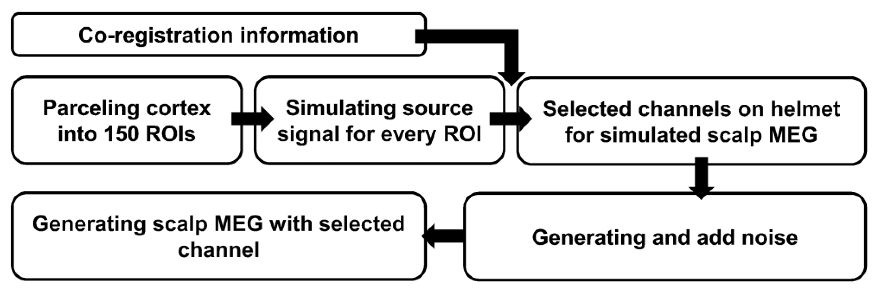
2.2. Simulation and MEG Experiments

The estimation of the cross-cortical gradient of spontaneous oscillations based on OPM-MEG is shown in Figure 2, which includes brain MRI segmentation and labeling, the acquisition of MEG and sensor co-registration, source reconstruction, oscillation parameterization, and the gradient estimation of parameterized oscillations.

2.2.1. Anatomical Coordinates of Regions of Interest (ROIs)

The anatomical images of participants’ heads were obtained with a Siemens MAGNETOM Prisma 3T MR system (Figure 2a). T1-weighted MRI scans were obtained with an MPRAGE sequence (TR, 2300 ms; TE, 3.03 ms; TI, 1100 ms; FA, 8; field of view, 256 mm × 256 mm × 192 mm; voxel size = 1.0 mm × 1.0 mm × 1.0 mm). MRI data were preprocessed and segmented with Freesurfer (versions 7) software [40] to obtain the scalp surface and cortex. The cortex surface was parceled into 150 ROIs (75 per hemisphere) with 5124 vertices, according to aparc.a2009s atlas [41]. And the coordinates $\left(x_i,y_i,z_i\right)$ of the center of mass of the $i$ ROIs were obtained.

2.2.2. Co-Registration Data and Forward Model

Participants wearing the helmet were 3D-scanned to obtain 3D images for the co-registration of OPM sensors and MRI data with a structure-light scanner (Occipital Inc., San Francisco, CA, USA). The sensor slots of the helmet are arranged according to the 10–20 EEG system. Co-registration included helmet match and face match [42,43]. The locations and orientations of sensors in slots relative to the head of a subject were obtained (Figure 2b).

The forward model was constructed with a Boundary Element Method (BEM) model [44] integrated with source spaces defined on the white matter surfaces of the superior cortex. Specifically, a single-layer BEM model with a conductivity of 0.3 S/m was constructed, and this model was used along with the source spaces (a total of 5124 source locations for the entire brain region of each subject) to build the forward model, consisting of 8196 sources with free orientations, which was established using the ‘make_forward_solution’ function from the MNE-Python toolkit [45]. This forward model allowed for the simulation of the magnetic fields generated by neural activity in the brain and used in cortical timeseries reconstruction.

2.2.3. Background Noise Data Acquisition

The background noise was acquired in a magnetically shielded room (MSR) (ambient-field amplitude and drift typically below 13 nT and 40 pT/h), without participants. Thirty-two dual-axis Gen-2 OPM sensors (QZFM, QuSpin Inc., Louisville, CO, USA) were arranged on a flexible helmet, which was securely positioned on a 3D-printed head phantom, ensuring comprehensive sensor coverage of the entire model. The preprocessing of this background noise data involved a 2–30 Hz bandpass filter and homogenous field correction (HFC) [46], both of which were executed using the MNE-Python [45].

2.2.4. Simulated MEG Signals

As depicted in Figure 3, the simulation of MEG signals was initiated after obtaining ROIs and co-registration information. Firstly, the ground true spatial gradient of PF (unit: Hz) and PT (unit: s) can be simulated according to Equation (1) for the $i$ ROI $\left(x_i,y_i,z_i\right)$ as follows.

$$P{F}_{\mathrm{ground},i}=10+0.002x_i-0.005y_i-0.001z_i-0.0001x_i{y}_i-7\times {10}^{-7}{x}_i{z}_i+2\times {10}^{-5}{y}_i{z}_i$$

(14)

$$P{T}_{\mathrm{ground},i}=2.5+0.001x_i-0.004y_i+0.005z_i-4\times {10}^{-5}{x}_i{y}_i-7\times {10}^{-5}{x}_i{z}_i+2\times {10}^{-5}{y}_i{z}_i$$

(15)

Then, the simulated gradient of PF and PT can be generated with ${\mathit{h}}_{\mathrm{sim}}~N\left({\mathit{h}}_{\mathrm{ground}},{\sigma }^2(\mathit{R}\mathit{D}{\mathit{R}}^{\mathrm{T}}+\mathit{I})\right)$. ${\mathit{h}}_{\mathrm{ground}}$ represents the ground values of PF and PT of all ROIs and simulated random groups. The simulated $\sigma$ of PF and PT were ${\sigma }_{\mathrm{PF}}=0.5\mathrm{Hz}$ and ${\sigma }_{\mathrm{PT}}=0.001\mathrm{s}$, respectively. The simulated $\mathit{D}$ of PF and PT were as follows.

$${\mathit{D}}_{\mathrm{PF}}=\mathrm{diag}\left(\mathrm{diag}({0.5}^2,{0.02}^2,{0.02}^2,{0.02}^2)\right)$$

(16)

$${\mathit{D}}_{\mathrm{PT}}=\mathrm{diag}\left(\mathrm{diag}({0.005}^2,{0.001}^2,{0.001}^2,{0.001}^2)\right)$$

(17)

The simulated number of random groups was 10 here. Finally, the simulated PF and PT of the $i^{\mathrm{th}}$ ROI can be obtained as $P{F}_{\mathrm{sim},i}$ and $P{T}_{\mathrm{sim},i}$ from ${\mathit{h}}_{\mathrm{sim}}$. The cortical source signal $st{c}_i\left(t\right)$ for the $i^{\mathrm{th}}$ ROI can be constructed as

$$st{c}_i\left(t\right)=a\times {10}^{-9}\sin \left(2.0\pi P{F}_{\mathrm{sim},i}\left(t-P{T}_{\mathrm{sim},i}/f_{\mathrm{s}}\right)\right)\exp {({\displaystyle \frac{t-P{T}_{\mathrm{sim},i}/f_{\mathrm{s}}}{t_{\mathrm{d}}/5}})}^2/2$$

(18)

where duration $t_{\mathrm{d}}$ of each oscillation was 3 s. $f_{\mathrm{s}}$ is the sampling frequency (1000 Hz in this paper). And the length of each signal is 7 s.

Then, we simulated the MEG with the MRI (Section 2.2.1) and co-registration data (Section 2.2.2) of one subject (28-year-old, male). In total, 16, 32, and 64 channels were selected according to the 10–20 EEG layout to simulate MEG recording for investigating the influence of the number of sensors. The forward model (8196 sources, free orientations) was updated with 16-, 32-, and 64-channel co-registration information. Then, ‘mne.simulation.simulate_raw’ in MNE-python [44] was used to generate the pure MEG data. And, noise was generated (with ‘mne.make_ad_hoc_cov’ in MNE-python) and added to pure MEG data (with ‘mne.simulation.add_noise’ in MNE-python), which is the white noise with a standard deviation of 15fT. For further quantifying the estimation performance of the cross-cortical gradient in a real experiment environment, the background noise was added to the pure MEG data with ‘compute_raw_covariance’ and ‘simulation.add_noise’ in MNE-python. The explanations of the above python functions are shown in

Table 1. The explanations for used functions from the MNE-python toolkit.

Functions	Explanations
mne.simulation.simulate_raw	To generate MEG data with source timeseries of all ROI.
mne.make_ad_hoc_cov	To quickly generate an ad hoc covariance matrix.
mne.simulation.add_noise	To add noise to simulated noise-free MEG data based on a noise covariance matrix.
compute_raw_covariance	To calculate a noise covariance matrix using empty room noise data.

.

2.2.5. SQUID-MEG Experiment

In this study, we used five minutes of resting-state MEG data from the MOUS dataset [47]. The participants were instructed to think of nothing specific with eyes open during MEG recording. Data were collected using a CTF 275channel SQUID-MEG system. The resting-state MEG data from 56 healthy participants (31 females, 25 males, mean age = 21.3 ± 1.5 years old) were utilized, after the exclusion of any abnormal data during preprocessing, forward model construction, and source reconstruction. The anatomical images of the head were obtained with a SIEMENS Trio 3T.

2.2.6. Participants of OPM-MEG Experiment

The inclusion criteria for volunteers primarily included individuals aged between 18 and 30, with no history of serious chronic illnesses, and no participation in other similar studies. The exclusion criteria encompassed those with cardiovascular and cerebrovascular diseases, those with diabetes, individuals currently taking medications that may affect neurological responses, those with implanted metallic materials (such as dental braces), or the presence of mental disorders. Additionally, volunteers who failed to complete the study tasks as required or experienced severe adverse reactions were excluded from the study. Ultimately, this study recruited data from six participants (two females, four males, mean age = 28 ± 0.9 years old).

2.2.7. EO-EC OPM-MEG Experiment

Participants kept their eyes open or closed for 8 s according to the voice command. In total, 54 epochs of each state were recorded for each participant. During the experiment, subjects were instructed to close or open their eyes in response to voice prompts and were given sufficient time (a 3 s interval) to complete the action. This approach mitigated the transient effects of light changes in the field of vision that occur at the moment of opening or closing the eyes, thereby minimizing their impact on MEG acquisition while ensuring that the subjects had time to adjust their states [48]. Furthermore, when dividing the trials, the time when the voice instruction began to play was not taken as the starting point of the resting state. Instead, the initial moment of each trial was set 2 s after the completion of the voice instruction, allowing sufficient time for participants to hear the instruction and respond accordingly. Prior to the formal experiment, participants underwent pre-instruction listening and adaptive training. The volume of the auditory stimulus was adjusted for each participant prior to the experiment to ensure a comfortable hearing and comprehension of the instructions, enabling them to respond promptly upon hearing the voice. The experiment was carried out in MSR, which was designed by Han et al. [49]. In total, 32 dual-axis Gen-2 OPM sensors were used to record MEG, covering over the whole head. The OPM sensors measured the brain magnetic field signals in the radial direction, enabling 32 channel data collections. And sensors were placed in MSR, which were fixed and arranged on the flexible helmet. After data acquisition, the OPMs were removed from the helmet. Co-registration was carried out for the sensor configuration [42,43], obtaining the locations and orientations of the sensors relative to the head of each subject.

The project was reviewed and approved by the Biomedical Ethics Committee of Beihang University (No. BM20200175) on 20 July 2020. All ethical regulations related to human experimentation, including the “Declaration of Helsinki”, were complied with. The experiment and photos were used with the consent and permission of the subjects.

2.2.8. MEG Data Preprocessing

The preprocessing process of MEG data consisted of abnormal trial removal, bandpass filtering (2–30 Hz), HFC, and an independent component analysis (ICA) [50]. These were carried out with MNE-python [45].

2.3. Cortical Timeseries Reconstruction

We compared the influence of several commonly used source reconstruction methods on resting-state MEG gradient estimation.

(1)

Minimum Norm Estimate (MNE) [51]: MNE estimates the current source distribution over the cortical surface based on the minimum norm criterion. It uses L2 regularization to suppress noise. It assumes that the energy of the source distribution is minimized while satisfying the measured magnetic or electric field data. MNE solves a linear inverse problem to estimate source strengths.

(2)

Linearly Constrained Minimum Variance (LCMV) [44]: The LCMV method aims to find a set of spatial filters that minimize the variance of the source estimates while satisfying the linear constraints imposed by the sensor data. Although the LCMV method itself does not directly apply regularization to the source current distribution, it indirectly achieves regularization effects by optimizing the design of the spatial filters.

(3)

Exact Low-Resolution Electromagnetic Tomography (eLORETA) [52]: eLORETA is a source localization technique based on the weighted least squares method that assumes a continuous distribution of source current density over the cortical surface with spatial correlations between adjacent source points. It estimates source current density by minimizing the energy of the source distribution while satisfying the measured data.

(4)

Dynamic Statistical Parametric Mapping (dSPM) [53]: dSPM combines statistical parametric mapping with source localization to detect and localize statistically significant source activities from MEG data. It estimates the source distribution using MNE or similar methods and then applies statistical tests to assess whether the activity at each source point is significantly different from noise levels. dSPM works by computing statistical significance maps for each source point, showing the degree to which source activity deviates significantly from baseline levels.

Based on the MRI data (see Section 2.2.1), co-registration data, and forward model (see Section 2.2.2), the inverse operator was assembled. Finally, the inverse operator was applied to MEG data to reconstruct source-level signals of ROIs with MNE-python. The relaxation parameter for the source space was set to 0.2. This parameter weighted the source variances of the dipole components that are parallel (tangential) to the cortical surface. The forward one was weighted (or normalized) with a depth prior, which was set to 0.8. It specified the depth weights to be used in calculating the inverse operation and was usually used to balance the accuracy of the depth with smoothness.

2.4. Parameterizing Transient Oscillation

The parameterization of spontaneous oscillations was achieved based on our proposed method STPPTO [21], which parameterized oscillations in the time–frequency domain (Figure 2f). In STPPTO, the Superlet transform was used to obtain a time–frequency spectrum of the cortical signal. Then, the time–frequency distribution of periodic activities was obtained from an aperiodic background in a time-resolved way. Each time-resolved aperiodic background fitting was performed across the entire 2–30 Hz spectrum with peak width limited between 2 and 10 Hz, a peak threshold of 1.5, and a maximum of 4 peaks. The definition of transient events was used to parameterize oscillations. Finally, the PF and PT of the spontaneous oscillations were obtained, including the PF, PT, and adjusted power defined as a multiple of the power of the aperiodic background.

2.5. The Evaluation Indexes

2.5.1. The Root Mean Square Error (RMSE)

The RMSEs of PF $RMS{E}_{\mathrm{PF}}$ and PT $RMS{E}_{\mathrm{PT}}$ in the simulation were defined as

$$RMS{E}_{\mathrm{PF}}=\sqrt{{\displaystyle \frac{1}{n}}{\sum }_i^n\left(P{F}_{\mathrm{ground},i}-P{F}_{\mathrm{e},i}\right)}$$

(19)

$$RMS{E}_{\mathrm{PT}}=\sqrt{{\displaystyle \frac{1}{n}}{\sum }_i^n\left(P{T}_{\begin{array}{c}ground,i\end{array}}-P{T}_{\mathrm{e},i}\right)}$$

(20)

where $P{F}_{\mathrm{ground},i}$ and $P{F}_{\mathrm{e},i}$ are the ground truth and estimated values based on Equation of PF in the gradient of the $i$ ROI, respectively. $P{T}_{\mathrm{ground},i}$ and $P{T}_{\mathrm{e},i}$ are the ground truth and estimated values based on Equation of PT in the gradient of the $i$ ROI, respectively.

2.5.2. The Correlation of Cross-Cortical Gradient Estimation Between Two MEG Data Results

If the fixed effect coefficients of the cross-cortical gradient estimation based on SQUID-MEG and EO OPM-MEG were ${\mathit{\beta }}_1$ and ${\mathit{\beta }}_2$, respectively, the correlation $r$ can be obtained on the same template brain (“fsaverage” template, parceled according to [41]) as follows. Firstly, the coordinates $\left(x_{\mathrm{tem},i},y_{\mathrm{tem},i},z_{\mathrm{tem},i}\right)$ of the $i^{\mathrm{th}}$ ROI in the “fsaverage” template can be obtained. Then, the estimated gradient based on OPM-MEG data can be expressed as $G_{1,i}=\left[1,x_{\mathrm{tem},i},y_{\mathrm{tem},i},z_{\mathrm{tem},i},x_{\mathrm{tem},i}{y}_{\mathrm{tem},i},x_{\mathrm{tem},i}{z}_{\mathrm{tem},i},y_{\mathrm{tem},i}{z}_{\mathrm{tem},i}\right]{\mathit{\beta }}_1$, while the estimated gradient based on SQUID-MEG data can be expressed as $G_{2,i}=\left[1,x_{\mathrm{tem},i},y_{\mathrm{tem},i},z_{\mathrm{tem},i},x_{\mathrm{tem},i}{y}_{\mathrm{tem},i},x_{\mathrm{tem},i}{z}_{\mathrm{tem},i},y_{\mathrm{tem},i}{z}_{\mathrm{tem},i}\right]{\mathit{\beta }}_2$. Thus, the correlation can be expressed as

$$r={\displaystyle \frac{{\sum }_{i=1}^{n_{\mathrm{ROI}}}\left(\left(G_{1,i}-\widetilde{G_1}\right)\left(G_{2,i}-\widetilde{G_2}\right)\right)/\left(n_{\mathrm{ROI}}-1\right)}{\sqrt{{\sum }_{i=1}^{n_{\mathrm{ROI}}}{\left(G_{1,i}-\widetilde{G_1}\right)}^2/\left(n_{\mathrm{ROI}}-1\right)}\sqrt{{\sum }_{i=1}^{n_{\mathrm{ROI}}}{\left(G_{2,i}-\widetilde{G_2}\right)}^2/\left(n_{\mathrm{ROI}}-1\right)}}}$$

(21)

where $n_{\mathrm{ROI}}=150$, which is the number of ROIs. $\widetilde{G_1}$ and $\widetilde{G_2}$ are $\left(\sum _{i=1}^n{G}_{1,i}\right)/n_{\mathrm{ROI}}$ and $\left(\sum _{i=1}^n{G}_{2,i}\right)/n_{\mathrm{ROI}}$, respectively.

3. Results

3.1. The Performance of Gradient Estimation on Simulated MEG

The performance of gradient estimation based on four commonly used source reconstruction methods and different-channel OPM-MEG was compared in the simulation, laying the base for subsequent gradient analyses of real data measured in EO-EC OPM-MEG experiments. As evinced in

Table 2. The $\mathit{R}\mathit{M}\mathit{S}{\mathit{E}}_{\mathrm{PF}}$ (Hz) of the gradient estimation.

Reconstruction Method	64 Channels	32 Channels	16 Channels	Mean
MNE *	0.54	0.44	0.29	0.42
LCMV *	0.26	0.33	0.37	0.32
eLORETA *	0.49	0.49	0.29	0.42
dSPM *	0.52	0.44	0.30	0.42
Mean (across methods)	0.45	0.43	0.31	-

* MNE: Minimum Norm Estimate. LCMV: Linearly Constrained Minimum Variance. eLORETA: Exact Low-Resolution Electromagnetic Tomography. dSPM: Dynamic Statistical Parametric Mapping.

, the RMSE pertaining to the estimation of peak frequency gradients $\mathit{R}\mathit{M}\mathit{S}{\mathit{E}}_{\mathrm{PF}}$, derived from simulated MEG data encompassing 16-, 32-, and 64-channel configurations, exhibits a small difference. The $\mathit{R}\mathit{M}\mathit{S}{\mathit{E}}_{\mathrm{PF}}$ with 32-channel configuration is lower (p < 0.05) than that of 64-channel configuration, and higher (p > 0.05) than that of 16-channel configuration. Meanwhile,

Table 3. The $\mathit{R}\mathit{M}\mathit{S}{\mathit{E}}_{\mathrm{PT}}$ (s) of the gradient estimation.

Reconstruction Method	64 Channels	32 Channels	16 Channels	Mean
MNE *	0.465	0.287	0.391	0.381
LCMV *	0.479	0.226	0.397	0.367
eLORETA *	0.470	0.307	0.382	0.386
dSPM *	0.465	0.289	0.392	0.382
Mean (across methods)	0.470	0.277	0.391	-

* MNE: Minimum Norm Estimate. LCMV: Linearly Constrained Minimum Variance. eLORETA: Exact Low-Resolution Electromagnetic Tomography. dSPM: Dynamic Statistical Parametric Mapping.

shows that the RMSE of the gradient estimation of PT $\mathit{R}\mathit{M}\mathit{S}{\mathit{E}}_{\mathrm{PT}}$ based on 32-channel simulated MEG is the smallest. The $\mathit{R}\mathit{M}\mathit{S}{\mathit{E}}_{\mathrm{PF}}$ with 32-channel configuration is lower (p < 0.05) than that of 16-channel configuration and 64-channel configuration. These results verified the feasibility of employing 32-channel sensors, OPM-MEG, for capturing the cross-cortical oscillation gradients.

Furthermore, the performance of the gradient estimation of peak frequency and peak time was quantified, based on the simulation data of real background noise.

Table 4. RMSE of the cross-cortical gradient estimation based on 32 channels containing real noise.

Reconstruction Method	RMSEPF (Hz)	RMSEPT (s)
MNE *	0.43	0.479
LCMV *	0.37	0.461
eLORETA *	0.42	0.480
dSPM *	0.42	0.479

* MNE: Minimum Norm Estimate. LCMV: Linearly Constrained Minimum Variance. eLORETA: Exact Low-Resolution Electromagnetic Tomography. dSPM: Dynamic Statistical Parametric Mapping.

demonstrates that the gradient estimation of PF is not influenced by background noise, while the gradient estimation of PT is influenced obviously. Additionally, as can be seen from Table 2, Table 3 and Table 4, four source reconstruction methods exhibit comparable effects on the cross-cortical gradient estimation of parameterized oscillations. Consequently, dSPM can be selected as the source reconstruction method (the gradient estimation results in Supplement Figure S1), aligning with the prevalent approach adopted in numerous studies analyzing neural activities derived from MEG data [53,54].

3.2. The Result of EC-EO OPM-MEG

The cortical timeseries of the resting state were constructed with dSPM. Then, PFs and PTs’ values were parameterized from the cortical timeseries using the STPPTO method. As illustrated in Figure 4a, the separated periodic time–frequency representations, averaged across 150 ROIs of some subjects, sub01, sub02, sub03, and sub04, demonstrate that the adjusted power of oscillations varies significantly across different resting states. Further, we compared the parameterized oscillation from the periodic time–frequency representation of all cortices, as shown in Figure 4b. It is evident that the PF in the eyes-closed OPM-MEG is mainly concentrated in the alpha band (10.54 ± 0.03 Hz), exhibiting a statistically significant difference compared to the eyes-open condition (p < 0.0001). Additionally, the PT in the closed-eye state (2.163 ± 0.023 s) also displays a marked difference from that of the open-eye state, with statistical significance (p < 0.01).

Subsequently, spatial gradients of PFs based on SQUID-MEG (Figure 5a) and OE OPM-MEG (Figure 5b) were obtained based on parameterized oscillations, cortical coordinates, and LMEM. To assess the consistency between these two modalities, we computed the correlation between the gradients of PFs captured by SQUID-MEG and OE OPM-MEG on the common ‘fsaverage’ brain template, employing Equation (13). This finding demonstrates a positive correlation (PF: r = 0.78, p < 0.001) between the frequency gradients of spontaneous brain oscillations measured by OPM-MEG in the open-eye state and those obtained via SQUID-MEG. This underscores the efficacy of OPM-MEG in precisely measuring frequency gradients in spontaneous brain activity, consistent with previous research findings.

Finally, the cross-cortical gradients of parameterized EO and EC spontaneous oscillations were calculated. Figure 6 shows the cross-cortical gradient of PF and PT of EO and EC spontaneous oscillations.

Table 5. Coefficients of the cross-cortical gradient of PF and PT of EO and EC spontaneous oscillations.

		$\mathbf{Intercept} {\widehat{\mathit{\beta }}}_{\mathit{i}\mathit{n}\mathit{t}}$	Slope
			${\widehat{\mathit{\beta }}}_1$	${\widehat{\mathit{\beta }}}_2$	${\widehat{\mathit{\beta }}}_3$	${\widehat{\mathit{\beta }}}_4$	${\widehat{\mathit{\beta }}}_5$	${\widehat{\mathit{\beta }}}_6$
EO	PF	12.71	−0.028	−0.016	0.019	−0.0006	0.0002	0.0004
	PT	2.376	−0.0014	0.0097	0.0052	−6.00 × 10−5	8.77 × 10−5	−5.08 × 10−5
EC	PF	10.46	−0.002	−0.001	0.002	−6.36 × 10−5	−9.18 × 10−7	−3.36 × 10−5
	PT	2.079	0.0008	−0.0020	0.0022	−1.96 × 10−6	−5.29 × 10−5	1.44 × 10−5

shows coefficients of linear mixed effect modeling of the cross-cortical gradient, which elucidates the relationship between PF or PT and the coordinates of the ROIs. Results showed that the peak frequency of spontaneous oscillations in the EC state was concentrated in the alpha band (Figure 6a). There was a significant negative correlation with changes in X- and Y-axis coordinates (p < 0.05) in the EC state, with a significant negative correlation with changes in Y-axis coordinates in the EO state, indicating a notable decrease in cortical activity along the posterior–anterior direction. Additionally, there is a marked negative correlation between the mixed effect of Y- and Z-axis coordinates and the gradient estimate of peak frequency (p < 0.05) (Table 5). The results indicated that the peak frequency of spontaneous oscillations decreases in cortical regions closer to the anterior and superior parts, implying slower oscillatory activity.

The spatial gradient of peak time of EC spontaneous oscillations also exhibited a significant negative correlation with Y-axis coordinates of the cortex (p < 0.05) (Figure 6b), indicating a decrease along the posterior–anterior direction (Figure 6b), while no significant correlation was observed in other directions. The mixed effect of Y- and Z-axis coordinates and the gradient estimate of peak time also show a clear negative correlation (p < 0.05) (Table 5), suggesting that the peak time of spontaneous oscillations occurs earlier in cortical regions closer to the anterior and upper part. In the EO state, the peak frequency of spontaneous oscillations is concentrated in both the alpha and beta bands. The peak frequency displays a negative correlation with the Y-axis, and the mixed effect of X- and Y-axis coordinates and the gradient estimate of peak frequency exhibit a pronounced negative correlation (p < 0.01), indicating that the frequency of spontaneous oscillations decreases and the fluctuation rate slows down in cortical regions closer to the anterior or right side. Similarly, the peak time in the open-eye state shows a negative correlation with the Y-axis, and the mixed effect of X- and Y-axis coordinates and the gradient estimate of peak frequency also exhibit a significant negative correlation (p < 0.01), suggesting that the peak frequency of spontaneous oscillations becomes smaller and the fluctuation rate slower in cortical regions is closer to the anterior or right side.

In summary, these results demonstrated that OPM-MEG can measure the gradient changes in spontaneous oscillations across cortical regions during the resting state, particularly from posterior to anterior regions. Moreover, the distinct oscillatory patterns observed between the open-eye and closed-eye resting conditions are elucidated through the perspectives of cross-cortical alterations in spontaneous oscillations (Figure 6 and Table 5), thereby validating that these differences pervade the entire brain, transcending the confines of the occipital lobe region alone.

4. Discussion

4.1. The Cross-Cortical Gradient of Spontaneous Oscillations

This paper investigates the cross-cortical gradient of spontaneous oscillations utilizing OPM-MEG for the very first time. Through simulations, this study quantifies the impact of prevalent OPM-MEG source reconstruction methodologies on the estimation of the gradient. Furthermore, it examines the influence of varying sensor counts on the gradient estimation. While results from 32- and 64-channel configurations exhibited comparable performance, the 16-channel setup notably suffered from compromised gradient estimation accuracy. Consequently, for researchers confronted with budgetary constraints and restricted to employing a limited number of sensors (such as less than 16), it is advised to focus on local gradient variations [54,55]. Some studies have been conducted on the gradient change in oscillatory activity in local functional areas. For instance, Wagstyl et al. found both increasing and decreasing gradients of thickness along the posterior–anterior axis for cortical layers in the somatosensory and motor cortex [56].These local gradients could also support the global gradient along the sensory to transmodal areas [57].

Moreover, this study compares the rhythmic gradients across the cortex during the resting state with eyes open and closed. It confirmed that the dominant peak frequency in the brain gradually varies along the posterior to anterior axis, following a global cortical hierarchy from early sensory to higher-order regions in both open-eye and closed-eye states. This study established a frequency gradient for spontaneous rhythms based on OPM-MEG, similar to the results of previous anatomical [57] and SQUID-MEG database-based [6,10] studies. It demonstrated that OPM-MEG can measure the gradient of spontaneous oscillations across cortical hierarchies. A distinguishing aspect of our study is the discussion on the relationship between the peak time of oscillatory activities and anatomical structures. The peak time was found to show an early-to-late pattern from the posterior to anterior direction and bottom to top direction of the brain during the EO state, while a late-to-early pattern was shown in the posterior to anterior direction during the EC state. Variations in rhythmic activities across anatomical structures may lead to the existence of temporally asynchronous but related oscillations between several different brain regions. For instance, Boto et al. measured resting-state functional connectivity with wearable OPM-MEG [58], which can be one of the explanations of the cross-cortical gradient of peak time. Urai and Donner found that neural oscillations mediate inter-cortical feed-forward and feedback interactions, and that such interactions can lead to phase-amplitude modulation between cortical layers [59]. In a memory test study, beta activity appeared first in the thalamus, followed by prefrontal and hippocampal synchronized beta [60].

Additionally, the cross-cortical gradient in the alpha band dominated in the closed-eye spontaneous oscillations, while the gradient of open-eye spontaneous oscillations included alpha and beta bands. It further verified that the difference in alpha bands between EO and EC states did not occur only in the occipital lobe but in the global cortex. Previous studies have demonstrated that variations in brain activity during open-eye and closed-eye behaviors are not limited to the occipital lobe [30], but also occur in other regions, as is inherent in human brain nature [34,61,62].

4.2. Limitations and Future Directions

Our results confirmed that the peak frequency and peak time of spontaneous oscillations follow a spatial gradient across the cortex. Moreover, OPM-MEG can measure this gradient. Our study also showed that there were differences in these gradients between open- and closed-eye states. However, there are some limitations. Firstly, the performance of the OPM-MEG acquisition system also influences the collection and analysis of the inter-cortical oscillation patterns. Due to limitations in source reconstruction technology, this paper has not fully leveraged the advantage of the multi-axial MEG signal acquisition capability of OPMs [63]. Additionally, constrained by costs and hardware systems, the monitoring and compensation of sensor movements during the acquisition process have not been implemented, which is a highly effective technique for enhancing the signal-to-noise ratio of brain magnetic signal acquisition [63,64]. Secondly, for complex information-processing activities in the brain [65], estimation with linear models seems to be inaccurate.

4.3. Future Directions

Aiming at the limitations of this study, there are some research directions for future exploration. Firstly, more advanced source reconstruction technologies [61], hardware noise reduction [66] techniques, and the utilization of OPM sensors [61,65,66] will significantly improve the reliability of collecting and analyzing inter-cortical oscillation patterns in the future. Secondly, multivariate non-linear regression methods may be required to obtain more accurate patterns of oscillations across cortical hierarchies, such as generalized additive models [67] and kernel regression [68] for complex information-processing activities in the brain. Additionally, as peak frequency and peak time are measures derived from brain activity, the gradients may be dynamically modulated depending on cognitive states, diseases, and aging, and even the group and number of participants. Furthermore, arranging more channels within the OPM-MEG system will significantly contribute to the reconstruction of more nuanced cortical timeseries, enabling a more intricate understanding of cortical regions. Hence, it is imperative to collect extensive data with sufficient statistical power to enhance and investigate the initial findings of this study.

5. Conclusions

In this paper, the cross-cortical gradient estimation of spontaneous oscillations was performed on resting-state OPM-MEG. The REML of the LMEM was used to estimate the cross-cortical gradient of parameterized spontaneous oscillations with open-eye and closed-eye resting-state OPM-MEG data. The results validated that OPM-MEG can measure frequency gradient changes in the posterior–anterior direction, especially the closed-eye alpha rhythms and open-eye alpha\beta rhythms. Furthermore, the cross-cortical gradient of peak time was analyzed for the first time. It was found that there was also a significant gradient of peak time across the cortex. In conclusion, this study provides a reference for conducting cross-cortical analyses of brain oscillatory fluctuations using OPM-MEG research data.

References

1. Paquola, C.; Wael, R.V.D.; Wagstyl, K.; Bethlehem, R.A.I.; Hong, S.-J.; Seidlitz, J.; Bullmore, E.T.; Evans, A.C.; Misic, B.; Margulies, D.S.; et al. Microstructural and Functional Gradients Are Increasingly Dissociated in Transmodal Cortices. PLoS Biol. 2019, 17, e3000284. [Google Scholar] [CrossRef] [PubMed]
2. Glasser, M.F.; Coalson, T.S.; Robinson, E.C.; Hacker, C.D.; Harwell, J.; Yacoub, E.; Ugurbil, K.; Andersson, J.; Beckmann, C.F.; Jenkinson, M.; et al. A Multi-Modal Parcellation of Human Cerebral Cortex. Nature 2016, 536, 171–178. [Google Scholar] [CrossRef] [PubMed]
3. Himberger, K.D.; Chien, H.-Y.; Honey, C.J. Principles of Temporal Processing Across the Cortical Hierarchy. Neuroscience 2018, 389, 161–174. [Google Scholar] [CrossRef]
4. Murray, J.D.; Bernacchia, A.; Freedman, D.J.; Romo, R.; Wallis, J.D.; Cai, X.; Padoa-Schioppa, C.; Pasternak, T.; Seo, H.; Lee, D.; et al. A Hierarchy of Intrinsic Timescales across Primate Cortex. Nat. Neurosci. 2014, 17, 1661–1663. [Google Scholar] [CrossRef]
5. Jasmin, K.; Lima, C.F.; Scott, S.K. Understanding Rostral–Caudal Auditory Cortex Contributions to Auditory Perception. Nat. Rev. Neurosci. 2019, 20, 425–434. [Google Scholar] [CrossRef]
6. Mahjoory, K.; Schoffelen, J.-M.; Keitel, A.; Gross, J. The Frequency Gradient of Human Resting-State Brain Oscillations Follows Cortical Hierarchies. eLife 2020, 9, e53715. [Google Scholar] [CrossRef] [PubMed]
7. Doelling, K.B.; Assaneo, M.F. Neural Oscillations Are a Start toward Understanding Brain Activity Rather than the End. PLoS Biol. 2012, 19, e3001234. [Google Scholar] [CrossRef]
8. Buzsáki, G.; Draguhn, A. Neuronal Oscillations in Cortical Networks. Science 2004, 304, 1926–1929. [Google Scholar] [CrossRef]
9. Kopell, N.J.; Gritton, H.J.; Whittington, M.A.; Kramer, M.A. Beyond the Connectome: The Dynome. Neuron 2014, 83, 1319–1328. [Google Scholar] [CrossRef]
10. Donoghue, T.; Haller, M.; Peterson, E.J.; Varma, P.; Sebastian, P.; Gao, R.; Noto, T.; Lara, A.H.; Wallis, J.D.; Knight, R.T.; et al. Parameterizing Neural Power Spectra into Periodic and Aperiodic Components. Nat. Neurosci. 2020, 23, 1655–1665. [Google Scholar] [CrossRef]
11. Keitel, A.; Gross, J. Individual Human Brain Areas Can Be Identified from Their Characteristic Spectral Activation Fingerprints. PLoS Biol. 2016, 14, e1002498. [Google Scholar] [CrossRef] [PubMed]
12. Zich, C.; Quinn, A.J.; Bonaiuto, J.J.; O’Neill, G.; Mardell, L.C.; Ward, N.S.; Bestmann, S. Spatiotemporal Organization of Human Sensorimotor Beta Burst Activity. eLife 2023, 12, e80160. [Google Scholar] [CrossRef] [PubMed]
13. Rhodes, N.; Rea, M.; Boto, E.; Rier, L.; Shah, V.; Hill, R.M.; Osborne, J.; Doyle, C.; Holmes, N.; Coleman, S.C.; et al. Measurement of Frontal Midline Theta Oscillations Using OPM-MEG. NeuroImage 2023, 271, 120024. [Google Scholar] [CrossRef] [PubMed]
14. Azanova, M.; Herrojo Ruiz, M.; Belianin, A.; Klucharev, V.; Nikulin, V. Resting-State Theta Oscillations and Reward Sensitivity in Risk Taking. Front. Neurosci. 2021, 15, 608699. [Google Scholar] [CrossRef] [PubMed]
15. Barry, R.J.; De Blasio, F.M. EEG Differences between Eyes-Closed and Eyes-Open Resting Remain in Healthy Ageing. Biol. Psychol. 2017, 129, 293–304. [Google Scholar] [CrossRef]
16. Leroy, S.; Major, S.; Bublitz, V.; Dreier, J.P.; Koch, S. Unveiling Age-Independent Spectral Markers of Propofol-Induced Loss of Consciousness by Decomposing the Electroencephalographic Spectrum into Its Periodic and Aperiodic Components. Front. Aging Neurosci. 2023, 14, 1076393. [Google Scholar] [CrossRef]
17. McSweeney, M.; Morales, S.; Valadez, E.A.; Buzzell, G.A.; Yoder, L.; Fifer, W.P.; Pini, N.; Shuffrey, L.C.; Elliott, A.J.; Isler, J.R.; et al. Age-Related Trends in Aperiodic EEG Activity and Alpha Oscillations during Early- to Middle-Childhood. NeuroImage 2023, 269, 119925. [Google Scholar] [CrossRef]
18. Lundqvist, M.; Miller, E.K.; Nordmark, J.; Liljefors, J.; Herman, P. Beta: Bursts of Cognition. Trends Cogn. Sci. 2024, 28, 662–676. [Google Scholar] [CrossRef]
19. Liang, X.; Wang, R.; Wu, H.; Ma, Y.; Liu, C.; Gao, Y.; Yu, D.; Ning, X. A Novel Time–Frequency Parameterization Method for Oscillations in Specific Frequency Bands and Its Application on OPM-MEG. Bioengineering 2024, 11, 773. [Google Scholar] [CrossRef]
20. Van Ede, F.; Quinn, A.J.; Woolrich, M.W.; Nobre, A.C. Neural Oscillations: Sustained Rhythms or Transient Burst-Events? Trends Neurosci. 2018, 41, 415–417. [Google Scholar] [CrossRef]
21. Brady, B.; Bardouille, T. Periodic/Aperiodic Parameterization of Transient Oscillations (PAPTO)–Implications for Healthy Ageing. NeuroImage 2022, 251, 118974. [Google Scholar] [CrossRef] [PubMed]
22. Shin, H.; Law, R.; Tsutsui, S.; Moore, C.I.; Jones, S.R. The Rate of Transient Beta Frequency Events Predicts Behavior across Tasks and Species. eLife 2017, 6, e29086. [Google Scholar] [CrossRef] [PubMed]
23. Pauls, K.A.M.; Nurmi, P.; Ala-Salomäki, H.; Renvall, H.; Kujala, J.; Liljeström, M. Human Sensorimotor Resting State Beta Events and Aperiodic Activity Show Good Test–Retest Reliability. Clin. Neurophysiol. 2024, 163, 244–254. [Google Scholar] [CrossRef] [PubMed]
24. Pei, H.; Pang, H.; Quan, W.; Fan, W.; Yuan, L.; Zhang, K.; Fang, C. Pulsed Optical Pumping in Electron Spin Vapor. Measurement 2024, 231, 114619. [Google Scholar] [CrossRef]
25. Brookes, M.J.; Leggett, J.; Rea, M.; Hill, R.M.; Holmes, N.; Boto, E.; Bowtell, R. Magnetoencephalography with Optically Pumped Magnetometers (OPM-MEG): The next Generation of Functional Neuroimaging. Trends Neurosci. 2022, 45, 621–634. [Google Scholar] [CrossRef]
26. Boto, E.; Holmes, N.; Leggett, J.; Roberts, G.; Shah, V.; Meyer, S.S.; Muñoz, L.D.; Mullinger, K.J.; Tierney, T.M.; Bestmann, S.; et al. Moving Magnetoencephalography towards Real-World Applications with a Wearable System. Nature 2018, 555, 657–661. [Google Scholar] [CrossRef]
27. Rier, L.; Rhodes, N.; Pakenham, D.; Boto, E.; Holmes, N.; Hill, R.M.; Rivero, G.R.; Shah, V.; Doyle, C.; Osborne, J.; et al. The Neurodevelopmental Trajectory of Beta Band Oscillations: An OPM-MEG Study. eLife 2024, 13. [Google Scholar] [CrossRef]
28. Cao, F.; Gao, Z.; Qi, S.; Chen, K.; Xiang, M.; An, N.; Ning, X. Realistic Three-Layer Head Phantom for Optically Pumped Magnetometer-Based Magnetoencephalography. Comput. Biol. Med. 2023, 164, 107318. [Google Scholar] [CrossRef]
29. Petro, N.M.; Ott, L.; Penhale, S.; Rempe, M.; Embury, C.; Picci, G.; Wang, Y.-P.; Stephen, J.M.; Calhoun, V.D.; Wilson, T.W. Eyes-Closed versus Eyes-Open Differences in Spontaneous Neural Dynamics during Development. NeuroImage 2022, 258, 119337. [Google Scholar] [CrossRef]
30. Zhang, X.; Chen, C.; Zhang, M.; Ma, C.; Zhang, Y.; Wang, H.; Guo, Q.; Hu, T.; Liu, Z.; Chang, Y.; et al. Detection and Analysis of MEG Signals in Occipital Region with Double-Channel OPM Sensors. J. Neurosci. Meth. 2020, 346, 108948. [Google Scholar] [CrossRef]
31. Ciulla, C.; Takeda, T.; Endo, H. MEG Characterization of Spontaneous Alpha Rhythm in the Human Brain. Brain Topogr. 1999, 11, 211–222. [Google Scholar] [CrossRef] [PubMed]
32. Barry, R.J.; Clarke, A.R.; Johnstone, S.J.; Magee, C.A.; Rushby, J.A. EEG Differences between Eyes-Closed and Eyes-Open Resting Conditions. Clin. Neurophysiol. 2007, 118, 2765–2773. [Google Scholar] [CrossRef]
33. Zhang, R.; Xiao, W.; Ding, Y.; Feng, Y.; Peng, X.; Shen, L.; Sun, C.; Wu, T.; Wu, Y.; Yang, Y.; et al. Recording Brain Activities in Unshielded Earth’s Field with Optically Pumped Atomic Magnetometers. Sci. Adv. 2020, 6, eaba8792. [Google Scholar] [CrossRef] [PubMed]
34. Feng, Y.-X.; Li, R.-Y.; Wei, W.; Feng, Z.-J.; Sun, Y.-K.; Sun, H.-Y.; Tang, Y.-Y.; Zang, Y.-F.; Yao, K. The Acts of Opening and Closing the Eyes Are of Importance for Congenital Blindness: Evidence from Resting-State fMRI. NeuroImage 2021, 233, 117966. [Google Scholar] [CrossRef]
35. Li, S.; Cai, T.T.; Li, H. Inference for High-Dimensional Linear Mixed-Effects Models: A Quasi-Likelihood Approach. J. Am. Stat. Assoc. 2022, 117, 1835. [Google Scholar] [CrossRef] [PubMed]
36. Maestrini, L.; Hui, F.K.C.; Welsh, A.H. Restricted Maximum Likelihood Estimation in Generalized Linear Mixed Models. arXiv 2024, arXiv:2402.12719. [Google Scholar]
37. McCulloch, C.E.; Searle, S.R.; Neuhaus, J.M. Generalized, Linear, and Mixed Models, 2nd ed.; Wiley: Hoboken, NJ, USA, 2008; ISBN 978-1-118-20996-7. [Google Scholar]
38. Laporte, F.; Charcosset, A.; Mary-Huard, T. Efficient ReML Inference in Variance Component Mixed Models Using a Min-Max Algorithm. PLoS Comput. Biol. 2022, 18, e1009659. [Google Scholar] [CrossRef]
39. Fischl, B. FreeSurfer. NeuroImage 2012, 62, 774–781. [Google Scholar] [CrossRef]
40. Destrieux, C.; Fischl, B.; Dale, A.; Halgren, E. Automatic Parcellation of Human Cortical Gyri and Sulci Using Standard Anatomical Nomenclature. NeuroImage 2010, 53, 1–15. [Google Scholar] [CrossRef]
41. Cao, F.; An, N.; Xu, W.; Wang, W.; Li, W.; Wang, C.; Yang, Y.; Xiang, M.; Gao, Y.; Ning, X. OMMR: Co-Registration Toolbox of OPM-MEG and MRI. Front. Neurosci. 2022, 16, 984036. [Google Scholar] [CrossRef]
42. Cao, F.; An, N.; Xu, W.; Wang, W.; Li, W.; Wang, C.; Xiang, M.; Gao, Y.; Ning, X. Optical Co-Registration Method of Triaxial OPM-MEG and MRI. IEEE Trans. Med. Imaging 2023, 42, 2706–2713. [Google Scholar] [CrossRef] [PubMed]
43. Jaiswal, A.; Nenonen, J.; Stenroos, M.; Gramfort, A.; Dalal, S.S.; Westner, B.U.; Litvak, V.; Mosher, J.C.; Schoffelen, J.-M.; Witton, C.; et al. Comparison of Beamformer Implementations for MEG Source Localization. NeuroImage 2020, 216, 116797. [Google Scholar] [CrossRef]
44. Gramfort, A.; Luessi, M.; Larson, E.; Engemann, D.A.; Strohmeier, D.; Brodbeck, C.; Parkkonen, L.; Hämäläinen, M.S. MNE Software for Processing MEG and EEG Data. NeuroImage 2014, 86, 446–460. [Google Scholar] [CrossRef]
45. Tierney, T.M.; Alexander, N.; Mellor, S.; Holmes, N.; Seymour, R.; O’Neill, G.C.; Maguire, E.A.; Barnes, G.R. Modelling Optically Pumped Magnetometer Interference in MEG as a Spatially Homogeneous Magnetic Field. NeuroImage 2021, 244, 118484. [Google Scholar] [CrossRef]
46. Schoffelen, J.-M.; Oostenveld, R.; Lam, N.H.L.; Uddén, J.; Hultén, A.; Hagoort, P. A 204-Subject Multimodal Neuroimaging Dataset to Study Language Processing. Sci. Data 2019, 6, 17. [Google Scholar] [CrossRef] [PubMed]
47. Hohaia, W.; Saurels, B.W.; Johnston, A.; Yarrow, K.; Arnold, D.H. Occipital Alpha-Band Brain Waves When the Eyes Are Closed Are Shaped by Ongoing Visual Processes. Sci. Rep. 2022, 12, 1194. [Google Scholar] [CrossRef] [PubMed]
48. Han, B.; Yang, J.; Zhang, X.; Shi, M.; Yuan, S.; Wang, L. A Magnetic Compensation System Composed of Biplanar Coils Avoiding Coupling Effect of Magnetic Shielding. IEEE Trans. Ind. Electron. 2023, 70, 2057–2065. [Google Scholar] [CrossRef]
49. Hyvarinen, A. Fast and Robust Fixed-Point Algorithms for Independent Component Analysis. IEEE Trans. Neural Netw. 1999, 10, 626–634. [Google Scholar] [CrossRef]
50. Hämäläinen, M.S.; Ilmoniemi, R.J. Interpreting Magnetic Fields of the Brain: Minimum Norm Estimates. Med. Biol. Eng. Comput. 1994, 32, 35–42. [Google Scholar] [CrossRef]
51. Pascual-Marqui, R.D.; Lehmann, D.; Koukkou, M.; Kochi, K.; Anderer, P.; Saletu, B.; Tanaka, H.; Hirata, K.; John, E.R.; Prichep, L.; et al. Assessing Interactions in the Brain with Exact Low-Resolution Electromagnetic Tomography. Philos. Trans. R. Soc. A Math. Phys. Eng. Sci. 2011, 369, 3768–3784. [Google Scholar] [CrossRef]
52. Dale, A.M.; Liu, A.K.; Fischl, B.R.; Buckner, R.L.; Belliveau, J.W.; Lewine, J.D.; Halgren, E. Dynamic Statistical Parametric Mapping: Combining fMRI and MEG for High-Resolution Imaging of Cortical Activity. Neuron 2000, 26, 55–67. [Google Scholar] [CrossRef]
53. Pesnot Lerousseau, J.; Parise, C.V.; Ernst, M.O.; van Wassenhove, V. Multisensory Correlation Computations in the Human Brain Identified by a Time-Resolved Encoding Model. Nat. Commun. 2022, 13, 2489. [Google Scholar] [CrossRef] [PubMed]
54. Power, L.; Bardouille, T. Age-related Trends in the Cortical Sources of Transient Beta Bursts during a Sensorimotor Task and Rest. NeuroImage 2021, 245, 118670. [Google Scholar] [CrossRef] [PubMed]
55. Beltrachini, L.; von Ellenrieder, N.; Eichardt, R.; Haueisen, J. Optimal Design of On-Scalp Electromagnetic Sensor Arrays for Brain Source Localisation. Hum. Brain Mapp. 2021, 42, 4869–4879. [Google Scholar] [CrossRef] [PubMed]
56. An, K.; Shim, J.H.; Kwon, H.; Lee, Y.-H.; Yu, K.-K.; Kwon, M.; Chun, W.Y.; Hirosawa, T.; Hasegawa, C.; Iwasaki, S.; et al. Detection of the 40 Hz Auditory Steady-State Response with Optically Pumped Magnetometers. Sci. Rep. 2022, 12, 17993. [Google Scholar] [CrossRef]
57. Wagstyl, K.; Larocque, S.; Cucurull, G.; Lepage, C.; Cohen, J.P.; Bludau, S.; Palomero-Gallagher, N.; Lewis, L.B.; Funck, T.; Spitzer, H.; et al. BigBrain 3D Atlas of Cortical Layers: Cortical and Laminar Thickness Gradients Diverge in Sensory and Motor Cortices. PLoS Biol. 2020, 18, e3000678. [Google Scholar] [CrossRef] [PubMed]
58. Huntenburg, J.M.; Bazin, P.-L.; Margulies, D.S. Large-Scale Gradients in Human Cortical Organization. Trends Cogn. Sci. 2018, 22, 21–31. [Google Scholar] [CrossRef]
59. Boto, E.; Hill, R.M.; Rea, M.; Holmes, N.; Seedat, Z.A.; Leggett, J.; Shah, V.; Osborne, J.; Bowtell, R.; Brookes, M.J. Measuring Functional Connectivity with Wearable MEG. NeuroImage 2021, 230, 117815. [Google Scholar] [CrossRef]
60. Zhang, H.; Watrous, A.J.; Patel, A.; Jacobs, J. Theta and Alpha Oscillations Are Traveling Waves in the Human Neocortex. Neuron 2018, 98, 1269–1281.e4. [Google Scholar] [CrossRef]
61. Wei, J.; Chen, T.; Li, C.; Liu, G.; Qiu, J.; Wei, D. Eyes-Open and Eyes-Closed Resting States with Opposite Brain Activity in Sensorimotor and Occipital Regions: Multidimensional Evidences From Machine Learning Perspective. Front. Hum. Neurosci. 2018, 12, 422. [Google Scholar] [CrossRef]
62. Jayachandran, M.; Viena, T.D.; Garcia, A.; Veliz, A.V.; Leyva, S.; Roldan, V.; Vertes, R.P.; Allen, T.A. Nucleus Reuniens Transiently Synchronizes Memory Networks at Beta Frequencies. Nat. Commun. 2023, 14, 4326. [Google Scholar] [CrossRef] [PubMed]
63. Rea, M.; Boto, E.; Holmes, N.; Hill, R.; Osborne, J.; Rhodes, N.; Leggett, J.; Rier, L.; Bowtell, R.; Shah, V.; et al. A 90-channel Triaxial Magnetoencephalography System Using Optically Pumped Magnetometers. Ann. N. Y. Acad. Sci. 2022, 1517, 107–124. [Google Scholar] [CrossRef] [PubMed]
64. Mellor, S.; Tierney, T.M.; OaNeill, G.C.; Alexander, N.; Seymour, R.A.; Holmes, N.; Lopez, J.D.; Hill, R.M.; Boto, E.; Rea, M.; et al. Magnetic Field Mapping and Correction for Moving OP-MEG. IEEE Trans. Biomed. Eng. 2022, 69, 528–536. [Google Scholar] [CrossRef] [PubMed]
65. Mellor, S.; Tierney, T.M.; Seymour, R.A.; Timms, R.C.; O’Neill, G.C.; Alexander, N.; Spedden, M.E.; Payne, H.; Barnes, G.R. Real-Time, Model-Based Magnetic Field Correction for Moving, Wearable MEG. NeuroImage 2023, 278, 120252. [Google Scholar] [CrossRef]
66. Holmes, N.; Rea, M.; Hill, R.M.; Leggett, J.; Edwards, L.J.; Hobson, P.J.; Boto, E.; Tierney, T.M.; Rier, L.; Rivero, G.R.; et al. Enabling Ambulatory Movement in Wearable Magnetoencephalography with Matrix Coil Active Magnetic Shielding. NeuroImage 2023, 274, 120157. [Google Scholar] [CrossRef]
67. Brookes, M.J.; Boto, E.; Rea, M.; Shah, V.; Osborne, J.; Holmes, N.; Hill, R.M.; Leggett, J.; Rhodes, N.; Bowtell, R. Theoretical Advantages of a Triaxial Optically Pumped Magnetometer Magnetoencephalography System. NeuroImage 2021, 236, 118025. [Google Scholar] [CrossRef]
68. Boto, E.; Shah, V.; Hill, R.M.; Rhodes, N.; Osborne, J.; Doyle, C.; Holmes, N.; Rea, M.; Leggett, J.; Bowtell, R.; et al. Triaxial Detection of the Neuromagnetic Field Using Optically-Pumped Magnetometry: Feasibility and Application in Children. NeuroImage 2022, 252, 119027. [Google Scholar] [CrossRef]
Figure 1. The flow of the estimation of D , β , and σ 2 .
Technologies 12 00254 g001
Figure 2. The estimation of cross-cortical gradient of spontaneous oscillations based on OPM-MEG, including MRI segmentation and reconstruction (a), sensors co-registration (b), the acquisition of MEG (c), ROIs parceling and source reconstruction (d), oscillation parameterization (f), and the gradient estimation of parameterized oscillations (e,f).
Technologies 12 00254 g002
Figure 3. Simulation of scalp MEG with simulated oscillatory gradient.
Technologies 12 00254 g003
Figure 4. The oscillations of all ROIs during closed-eye and open-eye states measured by OPM-MEG. (a) The separated periodic time–frequency representation average across 150 ROIs of subject sub01, sub02, sub03, and sub04. (b) The PF and PT values of closed-eye and open-eye OPM-MEG for all ROIs and all subjects.**** means p < 0.0001. ♦ means outlier points.
Technologies 12 00254 g004
Figure 5. The PF gradient of SQUID-MEG (a) and EO OPM-MEG (b) on the fsaverage brain template. Left panel: a cortical map of the cross-cortical gradient of PF on a template brain. Right panel: Dependency between the PF or PT and the ROI’s location along the y-axis (posterior to anterior).
Technologies 12 00254 g005
Figure 6. The cross-cortical gradient of peak frequency (a) and peak time (b) of EO and EC resting-state rhythmics. The upper panels of (a,b) show cortical maps of the cross-cortical gradient of EO and EC spontaneous oscillations on template brains. The bottom panels of (a,b) show the dependency between the PF or PT and cortex along the x-axis (left to right), the y-axis (posterior to anterior), and the z-axis (the bottom to the top), respectively. In (a,b), the dots show the original PFs or PTs obtained with STPPTO and the slopes show β ^ 1 , β ^ 2 , and β ^ 3 in Equation (13).
Technologies 12 00254 g006